A Two-Stage Seismic Damage Assessment Method for Small, Dense, and Imbalanced Buildings in Remote Sensing Images

Abstract

Large-scale optical sensing and precise, rapid assessment of seismic building damage in urban communities are increasingly demanded in disaster prevention and reduction. The common method is to train a convolutional neural network (CNN) in a pixel-level semantic segmentation approach and does not fully consider the characteristics of the assessment objectives. This study developed a machine-learning-derived two-stage method for post-earthquake building location and damage assessment considering the data characteristics of satellite remote sensing (SRS) optical images with dense distribution, small size, and imbalanced numbers. It included a modified You Only Look Once (YOLOv4) object detection module and a support vector machine (SVM) based classification module. In the primary step, the multiscale features were successfully extracted and fused from SRS images of densely distributed buildings by optimizing the YOLOv4 model toward the network structures, training hyperparameters, and anchor boxes. The fusion improved multi-channel features, optimization of network structure and hyperparameters have significantly enhanced the average location accuracy of post-earthquake buildings. Thereafter, three statistics (i.e., the angular second moment, dissimilarity, and inverse difference moment) were further discovered to effectively extract the characteristic value for earthquake damage from located buildings in SRS optical images based on the gray level co-occurrence matrix. They were used as the texture features to distinguish damage intensities of buildings, using the SVM model. The investigated dataset included 386 pre- and post-earthquake SRS optical images of the 2017 Mexico City earthquake, with a resolution of 1024 × 1024 pixels. Results show that the average location accuracy of post-earthquake buildings exceeds 95.7% and that the binary classification accuracy for damage assessment reaches 97.1%. The proposed two-stage method was validated by its extremely high precision in respect of densely distributed small buildings, indicating the promising potential of computer vision in large-scale disaster prevention and reduction using SRS datasets.

1. Introduction

As one of the most hazardous natural disasters, earthquakes have typical characteristics significantly different from other natural disasters, such as an instantaneous burst, unpredictability, destructiveness, complex mechanism, difficult defense, broad social impact, and quasi-periodic frequency. With the significant expansion of city population and rapid urbanization, earthquakes have undeniably become the main threat to buildings and other infrastructure in earthquake-prone areas [1]. According to the statistics of official departments, most of the casualties and economic losses after an earthquake are closely related to the destruction of buildings. Therefore, damage assessment of buildings plays a critical role in seismic damage surveys and emergency management of urban areas after an earthquake disaster. Scientists have conducted many investigations on earthquake occurrence mechanisms and disaster impacts for accurate disaster prevention and reduction.

Generally, the damage assessment of urban buildings after an earthquake needs two steps: object location and damage identification. Among those evaluation methods, the dynamic-response-based structural health monitoring method cannot conduct a comprehensive evaluation using signals collected by a limited number of sensors (e.g., an acceleration sensor), and the on-site ground survey, depending on the seismic experts or structural engineers, is mainly used to evaluate damage status [2]. Such a method needs to check the buildings one by one, making it challenging to overcome the limitations of accessible space and ineffective use of time. The assessment results greatly rely on the subjective judgment of surveyors, leading to the inevitable difficulty of guaranteeing detection stability due to the limited available information from manual visual observation (e.g., upper views and features of the buildings). Blind zones are also challenging to approach after an earthquake, given the possibity of secondary disasters. Therefore, highly accurate and rapid seismic damage assessment of urban buildings is increasingly demanded for the emergent response, effective searching, and quick rescue after an earthquake.

Comparatively, remote sensing, as a nearly emergent technology, has unique advantages, including a lack of contact, low cost, large-scale coverage, and fast response. Research communities have reported their attempts to use remote sensing data (e.g., optical or synthetic aperture radar (SAR) data)) for automatic seismic damage assessment and other fields [3,4,5,6]. The remote sensing method prioritizes earthquake damage assessment of buildings, and provides a much faster, more economical, and more compressive assessment than manual assessment. SAR data have become an all-weather information source for disaster assessment because of their strong penetration ability to disturbances, such as heavy clouds and rain [7,8,9,10]. Generally, most disaster assessments using SAR data are based on multi-source or multi-temporal data, which requires complex image registration and other necessary processes. To overcome these challenges, some researchers prefer satellite optical images [11]. Compared to SAR data, optical images are much easier to access and to process for extraction of the characteristic information of seismic damage. At present, building earthquake damage assessment based on satellite remote sensing (SRS) optical images mainly includes visual interpretation and change detection. These processes primarily rely on the graphical comparison pre- and post-earthquake, which shows unexpected limitations (e.g., it is challenging to obtain pre-images in less developed areas, and the assessment accuracy depends on technical expertise) and low efficiency [3,12].

Artificial intelligence (AI) has made explosive breakthroughs in recent years [13]. Essential methods of AI collection, machine learning (ML) and computer vision (CV) are mainly promoted by end-to-end learning through the use of artificial neural network (ANN) and CNN approaches. This supplies a new option that utilizes computers to process data and enables computers to analyze and interpret it. In recent years, many efficient algorithms have been created to promote the application of ML and CV methods in structural health monitoring [14,15,16,17,18,19,20,21,22,23]. These methods effectively reduce or eliminate the dependence on professional measuring equipment, expensive sensors, and the subjective experience of inspectors. AI/CV techniques can overcome the above shortcomings with high efficiency, stability, and robustness. Additionally, these techniques, merging with unmanned aerial vehicles and robotics, can assist humans to access the hard-to-inspect places and ensure safety. Therefore, AI/CV techniques are more suitable for rapid damage assessment of wide-area post-earthquake buildings [24,25]. Benefiting from the consistent improvements of remote sensing and AI technology, CV methods have been gradually developed for structural damage assessment, which mainly includes image classification, object detection, and semantic segmentation.

Fundamentally, single-stage object detectors, such as YOLO [26,27,28,29], and single-shot multibox detectors (SSDs) [30] omit the process for obtaining the proposal region and transforming the object detection task for location and classification into a regression problem. However, they present unsatisfactory adaptability for SRS data (e.g., low accuracy, either false or missing detection) because of apparently different characteristics rather than natural images, such as limited vertical view information, small and dense objects, complex environmental background, and illumination variation. However, their advantages, including high precision, small volume, and fast operation speed, are advisable for the rapid disaster assessment of urban buildings after an earthquake based on SRS optical images. Moreover, as seismic damage classification of urban buildings greatly depends on footprint information, the accuracy of building positioning directly affects the result of earthquake damage assessment. In most earthquake on-sites, it is challenging to realize ‘one-step’ damage assessment by the data-driven deep learning methods owing to the lack of high-quality annotation datasets [31]. Under the actual scenarios of investigated urban areas, most of the buildings in the SAR images are in normal condition, while only a few are damaged (which are actually concerned by post-earthquake disaster assessment). Therefore, it causes an imbalanced problem for damage severity classification, which is also a common problem in the field of structural health monitoring for civil engineering. It makes machine learning difficult because the model would be misguided by the overwhelming majority of normal samples and have limited recognition ability of damaged samples. Therefore, it is significant to investigate the problem caused by imbalanced data.

To solve the above-mentioned issues of currently reported methods, this study proposed a modified You Only Look Once (YOLOv4) object detection module and a support vector machine (SVM) derived classification module for building location and damage assessment. Specifically, the objectives of the paper are as follows:

(1)

This paper aims to develop a novel method for rapid and accurate wide-area post-earthquake building location and damage assessment using SRS optical images.

(2)

To detect tiny-sized and densely distributed buildings, the YOLOv4 model is improved to achieve a much higher precision.

(3)

To classify the damage severity of imbalanced buildings, images features of gray level co-occurrence matrix (GLCM) that can effectively distinguish different damage severities are extracted and utilized in SVM classification.

The remainder of this article is organized as follows. Section 2 focuses on the related work of damage assessment of post-earthquake buildings in SRS optical images using CV methods. Section 3 exhibits the dataset and experiment details. Section 4 introduces the overall framework of the proposed method. Section 5 describes the first module of building location and discusses the results. Section 6 explains the second module of post-earthquake damage classification and illustrates the results. Section 7 concludes the article.

2. Related Work

Research communities have introduced CV into building location and damage classification based on SRS optical images. Ci et al. [32] proposed a new CNN combined with ordinal regression, making full use of historical accumulated data. The results showed 77.39% accuracy of four classifications and 93.95% accuracy of two classifications for the 2014 Ludian earthquake. Duarte et al. [33] adopted SRS images with different resolutions from satellites and airborne platforms to achieve better accuracy in the damage classification of buildings by integrating multiscale information. Maggiori et al. [34] addressed the issue of imperfect training data through a two-step training approach and developed an end-to-end CNN framework for building pixel classification of large-scale SRS images. The approach was initialized on a large amount of possibly inaccurate reference data (from the online map platform) and then refined on a small amount of manual, accurately labeled data. Adriano et al. [35] realized the four-pixel-level classification of building damage with more accuracy than 90% after combining SRS optical data and SAR data. Liu et al. [36] demonstrated a layered framework for building detection based on a deep learning model. By learning building features at multiscale and different spatial resolutions, the mean average precision (mAP) of this model for building detection in SRS images was 0.57. To solve the gap between the axial detection box of conventional objects and the actual azimuth variation, Chen et al. [37] introduced directional anchors and additional dimensions, which achieved a mAP of 0.93 for object detection of buildings. Etten et al. [38] addressed a suitable model named You Only Look Twice for processing large-scale SRS images by modifying the You Look Only Once v2 (YOLOv2) structure with finer-grained features and a denser final grid, which achieved an F1-score of 0.61 for building detection. Ma et al. [39] replaced the Darknet53 in YOLOv3 with the Shufflenetv2 and adopted GIoU as the loss function. The results on SRS images with a resolution of 0.5 m for the Yushu and Wenchuan earthquakes showed that the modified model could detect collapsed buildings with a mAP of 90.89%.

There is a need for accurate and efficient machine learning models that assess building damage from SRS optical images. The xBD database [40] is a public, large-scale dataset of satellite imagery for post-disaster change detection and building damage assessment. It covers a diverse set of disasters and geographical locations with over 800,000 building annotations across over 45,000 km² of imagery. Furthermore, Gupta et al. [39] created a baseline model. The localization baseline model achieved an IoU of 0.97 and 0.66 for “background” and “building,” respectively. The classification baseline model achieved an F1-score of 0.663, 0.143, 0.009, and 0.466 for no damage, minor damage, major damage, and destroyed building classes, respectively.

Many researchers [40,41,42,43] began to use the xBD dataset as benchmark dataset for automated building damage assessment studies. Shao et al. [41] reported a new end-to-end remote sensing pixel-classification CNN to classify each pixel of a post-disaster image as an undamaged building, damaged building, or background. During the training, both pre- and post-disaster images were used as inputs to increase semantic information, while the dice loss and focal loss functions were combined to optimize the model for solving the imbalance problem. The model achieved an F1-score (a comprehensive index) of 0.83 in the xBD database with multiple types of disasters. Bai et al. [42] developed a new benchmark model called pyramid pooling module semi-Siamese network (PPM-SSNet), by adding residual blocks with dilated convolution and squeeze-and-excitation blocks into the network and compressing incentive to improve the detection accuracy. Results achieved a F1 score of 0.90, 0.41, 0.65, and 0.70 for four damage types, respectively.

It can be found that the common idea underlying these methods is to train a CNN in a pixel-level semantic segmentation approach [32,33,34,35,36,37,38,39,40,41,42,43]. For adjacent buildings or buildings with occlusion views, these methods cannot distinguish the geometric range of each independent building after the earthquake. Moreover, due to the influence of imbalanced data on model training, they generally exhibit lower accuracies for damaged samples. Therefore, it is significant to fully consider these characteristics of unbalanced, tiny-sized, and densely distributed buildings and develop an appropriate building recognition and damage assessment method.

3. Preparation of Urban Earthquake Dataset

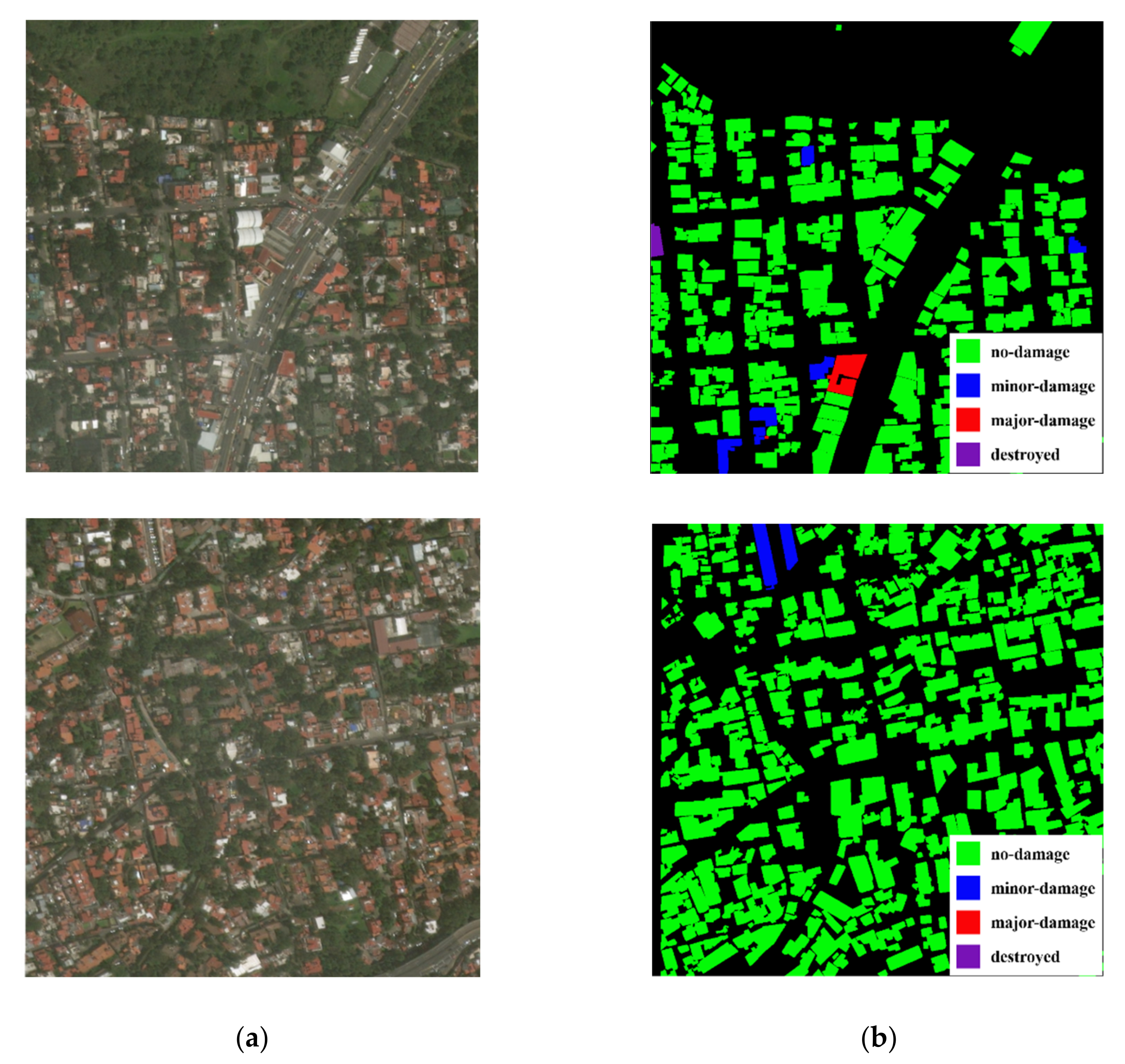
The 2017 Mexico City earthquake data from the xBD database [40] was adopted in this study. To conduct the large-scale post-earthquake damage assessment, 386 pre- and post-earthquake SRS images with a resolution of 1024 × 1024 pixels and a ground sampling distance of 0.8 m were selected. According to the joint damage rating established by the European macroseismic scale (EMS-98), the building damage was divided into four categories. Representative images are shown in Figure 1a, and the corresponding labels for the polygon location and damage categories of urban buildings are shown in Figure 1b. Green, blue, red, and purple represent no damage, minor damage, major damage, and destroyed, respectively.

Table 1. Descriptions and numbers of buildings for four damage categories in the original dataset.

Damage Category	Status Description of Damages	Number of Buildings
No damage	Undisturbed, no sign of structural damage	51,084
Minor damage	Roof missing, visible cracks	221
Major damage	Partial wall or roof collapses	54
Destroyed	Completely collapsed	3

shows the detailed descriptions of the damage categories and numbers of buildings in 193 post-earthquake SRS images. As illustrated in Figure 1 and Table 1, the selected dataset presented quite different characteristics than the natural images. For detection objects, buildings in satellite images showed a tiny observable size, dense distribution, and imbalanced damage types.

Furthermore, the number of buildings corresponding to the four damage categories was highly imbalanced; buildings with no damage far outnumbered those in the other three categories. Internal and facade information of buildings were also unable to assess post-earthquake damage other than directly viewed roofs comprehensively. In addition, the available SRS images mainly presented a unified resolution and single hue. Thus, the optimization of detector and classifier should be taken to make up for the shortage caused by the above-summarized data imperfection.

3.1. Data Preparation for Tiny Dense Object Detection of Post-Earthquake Buildings

A total of 386 pre- and post-earthquake images from the 2017 Mexico City earthquake dataset were collected for object detection of the post-earthquake buildings. The pre-earthquake images were regarded as data augmentation to increase the diversity of training sample space, while the corresponding damage was labeled as no damage. Moreover, reported studies have shown that the usage of both pre- and post-disaster images facilitates build location and damage classification after the earthquake [31,41]. Figure 2 shows the ground-truth bounding boxes of tiny, dense buildings in an SRS image using original polygon annotations of buildings. The minimal rectangular box surrounding each building was determined by the minimum and maximum coordinates of the polygon.

Considering the memory limit of the Graphics Processing Unit (GPU), the input size of the sub-images was adjusted as 608 × 608 pixels. A sliding window of 608 × 608 pixels with an overlap of 96 in width and height was used to generate patches from the original image of 1024 × 1024 pixels. Edge pixels were padded with pixel intensities of zero, and the 15% overlap area ensured that all regions would be analyzed. This strategy was also conducive to data augmentation by introducing translation to the edge images. Consequently, a total of 13,896 patches were obtained, among which 80% of the data was used for training, and the remaining 20% was used for testing. Statistical analysis showed that the modified dataset contained 1,317,237 buildings, while 95 buildings were included per patch on average.

As shown in Figure 3, the distribution histogram of building size (the square root of width × height) in the dataset showed that the number of object sizes ranged from pixels of 0–16, 16–32, 32–48, 48–64, 64–80, 80–96, and 96–608 are 13.24, 40.94, 25.97, 11.17, 4.60, 1.91, and 2.17%, respectively. According to the MS COCO dataset [44], the object scales could be divided into three typical types: the small object (<32 pixels), the medium object (32–96 pixels), and the large object (>96 pixels). The statistical results showed that more than half of building objects (54.18%) in this selected dataset were of the small-object type. Moreover, extremely tiny objects (<16 pixels) took up a proportion of 13%, making them more challenging to detect than normal small parts.

3.2. Data Preparation for Classification of Highly Imbalanced Damage

In general, SRS images can cover a vast area in a vertical view but little spatial information. For instance, when the ground floor of the building completely collapses with the superstructure remaining intact, it is difficult to identify such a damage status using satellite images. Therefore, most reported studies have only divided the buildings into two categories: not collapsed and collapsed [32,39,45]. In this study, buildings were first cropped to rectangular regions separately from the original image. They were then divided into two damage levels containing four different damage levels: no damage or minor damage (Class 1), and major damage or destroyed (Class 2). Class 1 defines reusable buildings after an earthquake, while Class 2 implies that the building is too severely damaged to reuse. All of the 57 major damage and destroyed buildings in Table 1 were classified as Class 2. Then, a dataset of no-damage and minor-damage buildings, with the same numbers of 57 as Class 1, was randomly selected. These 114 candidates constructed the dataset to train the SVM classifier for building damage classification. The training and testing sets included 70% and 30%, i.e., 40 and 17 samples for the two categories, respectively. Figure 4 visually depicts the examples for post-earthquake building damage classification. It shows that Class 1 (no damage and minor damage) had clear and intact geometric configurations. In contrast, the major damage and destroyed buildings in Class 2 had poor geometric integrity, vague edges, and scattered rubbles around them. Thus, different damage statuses could be distinguished from the irregular and disordered texture features using these images.

4. Framework

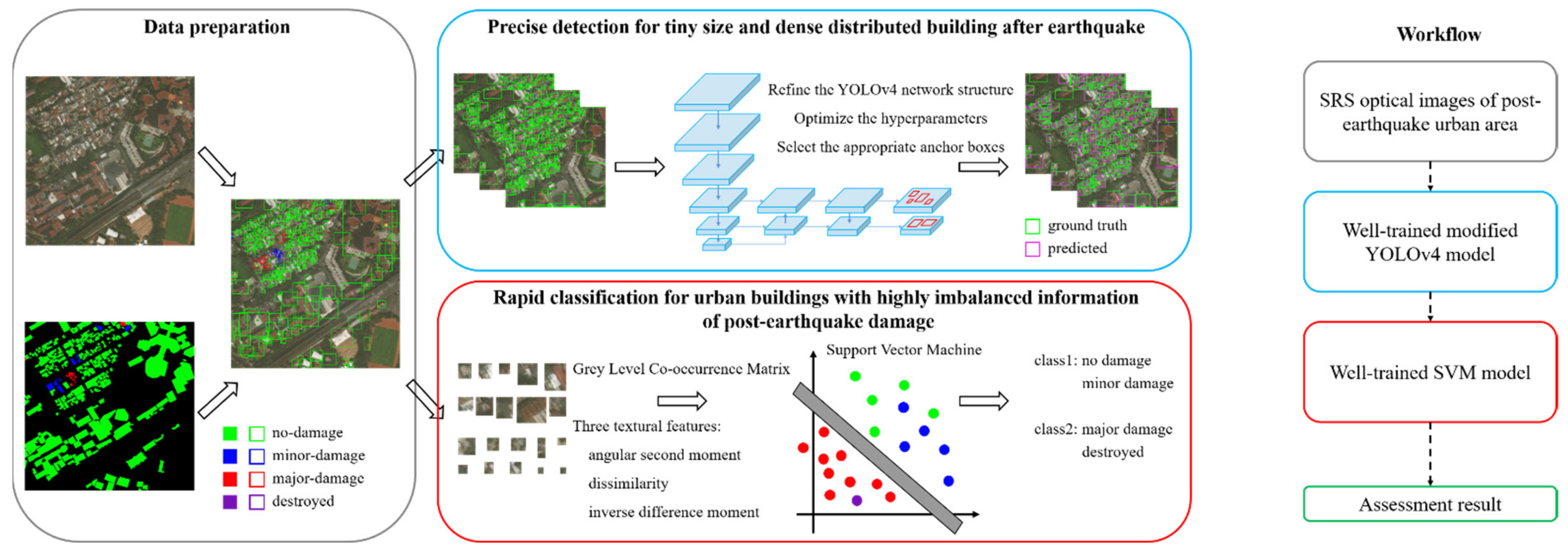
Considering the unique characteristics (tiny size, dense distribution, imbalanced information, and multiscale features) of SRS optical images for urban regions after earthquake disasters, we proposed a machine-learning-derived two-stage method enabling exact building location and rapid seismic damage assessment. In detail, the model was designed to collaboratively realize the detection and classification depending on two hybrid functional modules as a modified YOLOv4 and a support vector machine (SVM). The two-stage detection of YOLOv4 enables the precise detection and location of tiny dense buildings in SRS images, while the supervised-learning-based SVM offers a way for rapid classification using texture features of seismic damages. The schematic illustration and workflow of the proposed framework are shown in Figure 5. The proposed method consists of three modules, including data preparation, detection for buildings after an earthquake, and classification for buildings of post-earthquake damage:

(1)

Data preparation

The 2017 Mexico City earthquake dataset from the xBD database was selected, including SRS images for pre- and post-earthquake buildings and classification labels of damage intensities for building instances. A more detailed description is offered in Section 3.

(2)

Precise detection for tiny-sized and densely distributed buildings after an earthquake

To adapt the precise detection of tiny-sized and densely distributed buildings after urban earthquake utilizing SRS optical images, the YOLOv4 model was relevantly optimized by constructing a more efficient network, optimizing the hyperparameters, and selecting the more appropriate anchor boxes. After that, a well-trained YOLOv4 model was obtained for the precise location of buildings. The details of implementation can be found in Section 5.

(3)

Rapid classification for urban buildings with highly imbalanced information on post-earthquake damage

Six texture features with a single building in each detected bounding box were extracted by a gray level co-occurrence matrix (GLCM). Among them, three (i.e., the angular second moment, dissimilarity, and inverse difference moment) were validated as effective characteristics to support the following SVM that derived the binary classification of damage intensity (i.e., destroyed/major damage and minor damage/no damage). The detailed discussion is set out in Section 6.

The workflow is shown in the right part of Figure 5. After the SRS optical images of post-earthquake buildings in urban areas are input to the modified YOLOv4 model, rectangular bounding boxes are generated for the buildings. Consequently, each image patch inside the generated bounding box is used to obtain the GLCM features and then utilized as the input of the well-trained SVM classification model. Finally, the damage level is classified for each building inside the SRS image.

5. Small, Dense Object Detection of Post-Earthquake Buildings

5.1. Introduction of the Original YOLOv4 Model

Deep-learning-based object detection methods have been extensively proposed since 2014 [46], among which YOLO is a widely used single-stage end-to-end model that has evolved four generations. YOLOv4 has achieved state-of-the-art performance in the object detection field, and it has achieved a detection accuracy of 43.5% and a speed of 65 FPS in the MS COCO dataset [44]. Therefore, YOLOv4 holds promising potential for detecting post-earthquake buildings owing to its high precision and rapid speed. Figure 6a clearly describes the structure of the YOLOv4 object detector; it comprises three parts: the backbone, neck, and head:

• The backbone part comprises CSPDarknet53; it conducts downsampling in CSP1, CSP2, CSP8, CSP8, and CSP4 modules by 2, 4, 8, 16, and 32 times, respectively. The feature layer with 32 times downsampling has rich feature dimensions and a large receptive field, but the feature scale is compressed seriously, which is more suitable for object detection with large size. In contrast, the eight times downsampling is appropriate for small objects, obtaining a larger feature scale, a smaller feature dimension, and a receptive field. Comparatively, the 16 times downsampling located in the middle of the two layers prefers to detect the medium objects.
• The neck part is composed of PANet [47] and SPP additional modules [48]. PANet fuses features from different backbone scales for different detector scales. The SPP module is used to increase the receptive field of the backbone and separate the significant context features;
• The head part is a multi-head structure in three scales, in which a total of 9 anchor boxes are utilized to complete detection at multiscale. Eventually, the prediction bounding box with the highest confidence is retained by non-maximum suppression [49].

The YOLOv4 model uses a synthetical loss function, as follows:

$$Loss={\lambda }_{loc}Los{s}_{loc}+{\lambda }_{conf}Los{s}_{conf}+{\lambda }_{cls}Los{s}_{cls},$$

(1)

$$Los{s}_{loc}={\displaystyle \sum _{i=0}^{S^2}{\displaystyle \sum _{j=0}^B{1}_{ij}^{obj}{L}_{CIoU}}},$$

(2)

$$Los{s}_{conf}={\displaystyle \sum _{i=0}^{S^2}{\displaystyle \sum _{j=0}^B{1}_{ij}^{obj}{\left(C_i^j-{\widehat{C}}_i^j\right)}^2+}}{\displaystyle \sum _{i=0}^{S^2}{\displaystyle \sum _{j=0}^B{1}_{ij}^{noobj}{\left(C_i^j-{\widehat{C}}_i^j\right)}^2}},$$

(3)

$$Los{s}_{cls}=-{\displaystyle \sum _{i=0}^{S^2}{\displaystyle \sum _{j=0}^{B^2}{1}_{ij}^{obj}{\displaystyle \sum _{c\in classes}\left[{\widehat{p}}_i^{j}log\left(p_i^j\right)+\left(1-{\widehat{p}}_i^j\right)log\left(1-p_i^j\right)\right]}}},$$

(4)

where Loss_loc, Loss_conf, and Loss_cls denote the location, confidence, and classification losses, respectively. ${\lambda }_{loc}$, ${\lambda }_{conf}$, and ${\lambda }_{cls}$ are the corresponding penalty coefficients of the location loss, confidence loss, and classification loss, respectively. $1_{ij}^{obj}$ and $1_{ij}^{noobj}$ are binary indicator functions, representing whether the jth anchor box of the ith grid has an object (= 1) or not (= 0). S and B denote the numbers of grids and anchor boxes, respectively. $1_{ij}^{obj}$ and $1_{ij}^{noobj}$ are binary indicator functions, representing whether the jth anchor box of the ith grid has an object (= 1) or not (= 0), respectively. $C_i^j$ and ${\widehat{C}}_i^j$ are the confidence of the actual category and the predicted category of the jth anchor box of the ith grid, respectively. $p_i^j$ and ${\widehat{p}}_i^j$ are the classification accuracy of the real and the predicted category of the jth anchor box of the ith grid, respectively.

The CIoU [49] is used by considering the overlap area (IoU), distance from the center points (ρ²), and aspect ratios (w/h) of the predicted and ground-truth boxes, as follows:

$$L_{CIoU}=1-IoU+\frac{{\rho }^2(b,b^{gt})}{c^2}+\alpha \upsilon ,$$

(5)

$$IoU=\frac{B\cup B^{gt}}{B\cap B^{gt}},\upsilon =\frac{4}{{\pi }^2}{(arctan\frac{w^{gt}}{h^{gt}}-arctan\frac{w}{h})}^2,\alpha =\frac{\upsilon }{(1-IoU)+\upsilon },$$

(6)

where ${\rho }^2(b,b^{gt})$ represents the center distance between the predicted and ground-truth boxes. $B$ and $B^{gt}$ are the predicted and ground-truth boxes. $b$, $w$, $h$, $b^{gt}$, $w^{gt}$, and $h^{gt}$ denote the center coordinates, width, and height of the bounding (anchor) box, respectively. c denotes the diagonal length of the smallest enclosing box covering $B$ and $B^{gt}$.

5.2. Design of Modified YOLOv4 Model

To satisfy the specific characteristics of our SRS dataset rather than natural images, the YOLOv4 model was designed based on the profound modification of the original YOLO model. Figure 6b clearly describes the network structure of the modified YOLOv4 model.

• The backbone part remains the CSPDarkNet53 backbone feature extraction network. Thus, its 32 times downsampling layer retains high-level semantic information for later PANet modules to fuse multiscale information. In addition, the pre-trained weights of the backbone feature extraction network enable us to obtain the basic information of the image that can be used to transfer learning and fine-tuning.
• In the neck part, the PANet was optimized by removing the SPP module because it was verified to be useless in improving accuracy. However, many characteristic features will be lost for objects at small scales (<32 pixels) after 32 times downsampling. The 32 times downsampling layer in the PANet module was removed accordingly. Considering the usage of fixed-size images in the training phase, CBL*3 + SPP + CBL*3 was updated as CBL*5.
• In the head part, we retained and further optimized functions enabling both small and medium object detection at multiscale. The number of anchor boxes for the YOLO head correspondingly increased to the optimal number, which is conducive to matching more positive samples for medium and small objects to participate in loss calculation during training. Such improvements make the network more focused on specifically designed detection purposes.

5.3. Results and Discussion

Fundamentally, the performance of deep CNNs is highly dependent on the hyperparameter selection and network structure. For object detection, the choice of anchor box further affects the detection accuracy. Therefore, the effects of hyperparameters, network structures, and anchor boxes were systematically investigated and discussed. In reference to previously reported research, the pre-trained weights obtained from the large dataset should be capable of extracting the low-level and intermediate features of images [50]. Therefore, this study adopted the pre-trained weights on the MS COCO datasets and then conducted the necessary fine-tuning to make them suitable for our datasets.

Besides the evaluation index of IoU, widely used evaluation metrics, including precision, recall, F1-score, and mAP, were also utilized and defined as Equations (7)–(11):

$$Precision=\frac{TP}{TP+FP},$$

(7)

$$Recall=\frac{TP}{TP+FN},$$

(8)

$$F1-score=\frac{2\times Precision\times Recall}{Precision+Recall},$$

(9)

$$AP=\frac{1}{11}{\displaystyle \sum _{r\in \left[0,0.1,\dots 0.9,1\right]}\underset{\tilde{r}:\tilde{r}\ge r}{max}}(P(\tilde{r})),$$

(10)

$$mAP=\frac{{\displaystyle \sum _{i=1}^{N}A{P}_i}}{N},$$

(11)

where TP, FP, and FN are true positives, false positives, and false negatives, respectively. $P(\tilde{r})$ represents the measured precision at recall $\tilde{r}$ in the precision/recall curve. N is the number of categories, which equaled 1 in this study.

In the seismic damage assessment of buildings, accurate object identification and location is the basis of damage assessment. In general, the better training results should have a larger number of correct detections (TP) and fewer missed detections (FN). In addition, IoU measures the overlap rate between the predicted and ground-truth bounding boxes, which ranges from 0 to 1. A specific threshold needs to determine whether the predicted box localizes the correct object. As referred to in previously reported literature, the 0.5 IoU-based mAP has become the measuring standard for object detection problems for years [46], so it was also selected in this study.

5.3.1. Hyperparameter Investigations

The default hyperparameter configuration of YOLOv4 [29] has achieved excellent performance on the MS COCO dataset and is chosen as the basis for hyperparameter optimization. For instance, the stochastic gradient descent algorithm, with momentum m = 0.949, was used to update the network optimizer, and the initial learning rate was 0.001, with warm-up steps of 1000 iterations (as shown in Equation (12)).

$$initiallearningrate=0.001\times {(\frac{iterations}{1000})}^4,iterations\le 1000,$$

(12)

The mosaic method was applied to enhance the data to enrich the characteristic information in eigenspace. In detail, four training images were selected to form one image by random cutting, stitching, and arrangement. The background of detecting objects and the number of small objects could significantly increase. As a result, the demand for mini-batch was reduced, which could effectively improve the recognition effect of tiny objects. The relevant parameters for data enhancement are saturation = 1.5, exposure = 1.5, and hue = 0.1 at the input terminal, denoted by adjusting saturation, exposure, and hue to generate more training samples. In addition, the penalty coefficients of ${\lambda }_{loc}$, ${\lambda }_{conf}$, and ${\lambda }_{cls}$ losses in Equations (2)–(4) were 0.07, 1.0, and 1.0, respectively.

Next, considering the training efficiency, hyperparameters with a good model performance were retained for subsequent optimization during the ablation experiment. Some critical hyperparameters were investigated, including the size of the input image, batch parameters (batch size and subdivisions), number of iterations, learning rate strategy (steps and scales), and weight decay.

Table 2. Hyperparameter settings for different cases.

Case	Network Structure	Size of Input Image	Batch Size, Subdivisions	Number of Iterations	Steps	Scales	Weight Decay
1	YOLOv4 baseline	256	64, 16	4000	3200, 3600	0.1, 0.1	0.0005
2	YOLOv4 baseline	512	64, 16	4000	3200, 3600	0.1, 0.1	0.0005
3	YOLOv4 baseline	608	64, 16	4000	3200, 3600	0.1, 0.1	0.0005
4	YOLOv4 baseline	608	512, 128	4000	3200, 3600	0.1, 0.1	0.0005
5	YOLOv4 baseline	608	1024, 256	4000	3200, 3600	0.1, 0.1	0.0005
6	YOLOv4 baseline	608	512, 128	4000	3200, 3600	0.1, 0.1	0.1
7	YOLOv4 baseline	608	512, 128	4000	3200	0.1	0.1
8	YOLOv4 baseline	608	512, 128	8000	6400	0.1	0.1
9	Proposed	608	512, 128	8000	6400	0.1	0.1
10	Proposed	608	512, 128	10,000	8000	0.1	0.1

and

Table 3. Model performances under different hyperparameter settings.

Case	mAP	Precision	Recall	F1-Score	TP	FP	FN	Average IoU	Training Time (h)
1	41.5%	0.40	0.51	0.45	42,609	63,299	40,150	28.1%	1.2
2	72.5%	0.64	0.73	0.68	102,524	57,623	37,670	47.7%	4.4
3	79.6%	0.73	0.78	0.76	210,579	75,964	59,815	56.4%	6.7
4	89.3%	0.84	0.87	0.86	236,273	43,703	34,121	68.3%	57.2
5	90.3%	0.85	0.88	0.87	239,203	41,245	31,191	69.6%	111.2
6	92.3%	0.90	0.90	0.90	244,309	28,514	26,085	74.6%	57.5
7	93.2%	0.91	0.91	0.91	246,994	25,461	23,400	76.1%	57.4
8	95.2%	0.94	0.94	0.94	253,870	16,996	16,524	80.8%	116.5
9	95.7%	0.95	0.95	0.95	255,823	14,631	14,571	82.6%	120.5
10	95.8%	0.95	0.95	0.95	256,652	14,751	13,742	82.2%	154.6

show the specific hyperparameter settings and the corresponding model performance, respectively.

Cases 1, 2, and 3 in Table 3 indicate that the size of input images had a significant effect on the model performance. Multiple downsampling processing occurrences through the backbone feature extraction network generated a feature map reduced by 32 times, making it difficult for the network to capture the feature information of tiny objects. This indicates that the robustness of the detection model for small objects can be improved by inputting the larger size images for training.

Cases 3, 4, and 5 in Table 3 reveal that the increase in batch size can greatly improve performance within a specific range, and similar results have also been proposed by Goyal [51] and Keskar [52]. However, the longer training time slightly improves beyond a certain threshold. For instance, compared with case 4, case 5 gained only a 1% performance improvement but took nearly twice the training time. The subdivisions represent the mini-batch number of inputs owing to the memory limitation of GPU. Considering the training efficiency comprehensively, the size of the input image, batch size, and subdivisions were set as 608 × 608, 512, and 128, respectively.

In general, the regularization process can improve the generalization ability of the model and suppress overfitting. Adding the regular term $\frac{1}{2}\lambda {‖\omega ‖}^2$ ($‖\omega ‖$ denotes the 2-norm of network parameters) to the original loss function can affect the network during the error backpropagation process, and weight decay $\lambda$ is the coefficient of the regularization term. Cases 4 and 6 in Table 3 demonstrate the significant improvement of the model performance by increasing the weight decay within a specific range.

As another essential parameter, the learning rate determines the updating speed of the model. Typically, a too-large learning rate may cause the network to exceed the optimal value or even fail to converge. Otherwise, it has a slow convergence speed and can easily to fall into the local optimal value. The most used learning rate attenuation strategy selects a slightly larger learning rate at the beginning of the iteration, which gradually reduces with the increase of iterations. In this study, we chose a staged decay learning rate strategy with an initial value of 0.001. In Table 2, steps and scales equal the specified number of iterations and the multiplication factor of the current learning rate. The default learning rate in YOLOv4 was decayed in the form of a “two-phase type,” which decreased by 0.1 at 0.8 and 0.9 times of the total number of iterations, respectively. For example, Case 6 attenuated the learning rate to 0.0001 and 0.00001 at 3200 and 3600 iterations, respectively. Cases 6 and 7 in Table 3 show that the performance of the “one-phase type” was better than that of the “two-phase type”.

As a result, cases 7 and 8 in Table 3 show that increasing the total number of iterations significantly enhanced mAP. This was also validated by cases 9 and 10. However, when the total number of iterations increased from 8000 to 10,000 using the proposed network structure, it required nearly 30% of the extra training time for only 0.1% improvement in mAP. Therefore, the number of iterations, steps, and scales were set as 8000, 6400, and 0.1, respectively.

5.3.2. Optimization of Network Structure

Four different networks were designed to further optimize the performance of YOLOv4 on tiny dense object detection by multiscale networks, as shown in Figure 7. Briefly, structure-1 removed 32-times downsampling layers in the backbone and corresponding layers in the neck, and built a two-scale detector with 4 anchor boxes in the head (Figure 7a). Structure-2 changed the 8-times downsampling layers to four times, and further connected with 16 times in the neck. In addition, structure-2 selected a three-scale detector with three anchor boxes at the corresponding scale in the head (Figure 7b). Structure-3 detached both 32 and 16 times of downsampling layers in the neck and designed a one-scale detector with nine anchor boxes in the head (Figure 7c). In comparison, structure-4 removed 32 times of downsampling layers in the neck and added a two-scale detector with four anchor boxes in the head (Figure 7d).

Table 4. Specific details for four different network structures.

Network Structure	Scales of the Downsampling Sampling Layers in the Backbone	Scales of the Downsampling Sampling Layers in the Neck	Number of the YOLO Head
Structure-1	2, 4, 8, 16	8, 16	2
Structure-2	2, 4, 8, 16, 32	4, 16, 32	3
Structure-3	2, 4, 8, 16, 32	8	1
Structure-4	2, 4, 8, 16, 32	8, 16	2

demonstrates the differences among the proposed networks, which included the downsampling sampling layers at different scales in the backbone and neck, and the numbers of YOLO heads. The related hyperparameter settings are listed in

Table 5. Hyperparameter settings for four different network structures of modified YOLOv4.

Case	Network Structure	Batch Size	Subdivisions	Number of the Head	Number of Anchor Boxes per Head	Number of Clustering Centers
11	YOLOv4 baseline	512	128	3	3	9
12	structure-1	512	128	2	4	8
13	structure-2	512	256	3	3	9
14	structure-3	512	128	1	9	9
15	structure-4	512	128	2	4	8
16	proposed	512	128	2	4	8

. Moreover, the size of the input image was 608 × 608, the weight decay was 0.1, the learning rate was in the form of “one-phase type,” and the total number of iterations was 4000.

Table 6. Model performances of four different network structures of modified YOLOv4.

Case	mAP	Precision	Recall	F1-Score	TP	FP	FN	Average IoU	Training Time (h)	Model Size (M)
11	92.5%	0.89	0.91	0.90	245,597	29,260	25,797	74.4%	63.5	256.0
12	92.1%	0.91	0.90	0.90	242,066	23,082	28,328	75.9%	56.8	69.6
13	92.7%	0.91	0.89	0.90	241,604	23,815	28,790	75.8%	162.4	256.0
14	93.0%	0.93	0.90	0.91	242,879	17,956	27,515	77.9%	80.7	171.3
15	93.0%	0.91	0.91	0.91	245,063	22,841	25,331	76.8%	61.0	188.2
16	93.3%	0.92	0.91	0.92	246,268	19,975	24,126	77.9%	56.5	184.0

systematically illustrates the various performances of different network structures. Among these modified YOLOv4 networks, the mAP of structure-1 was even lower than that of the primary network. This reveals that the high-level semantic information in the 32 times downsampling layers of backbone feature extraction network plays a significant role in tiny, dense object detection. Comparatively, finer-grained features extracted by the four times downsampling layers in the neck of structure-2 contributed to the performance improvement, but the increased network size made it only suitable for batch parameters of 512 and 256 using the same GPU. This indicates that the mediocre performance still needs a relatively long time consumption. After that, we investigated the multiscale detectors in the head on the tiny dense object detection without changing the backbone. Cases 14 and 15 in Table 6 maintained small-scale (and medium-scale) detectors in the head, which was more suitable for the characteristics of our dataset. The results showed the same mAP performance of structure-3 and structure-4, but structure-4 presented a 0.9% increase in TP and a 7.9% reduction in FN. This validated that a two-scale detector covering medium and tiny scales in structure-4 is more likely to extract characteristic features from our SRS dataset. Moreover, compared with the original YOLOv4 model, the proposed structure (structure-4 without SPPNet) archived optimal performance with the training time, and the well-trained model size dropped by 11% and 28% under the same hyperparameters, respectively. This indicates that the inference efficiency for SRS images is effectively improved using the lightweight model.

5.3.3. Investigation of Prior Anchor Box

Since it was first proposed by Ren et al. in Faster R-CNN [53], the anchor box has been widely applied in object detection models. Appropriate setting of prior anchor boxes enhances model performance and reduces inference efficiency. Theoretically, the size of the anchor boxes can be obtained by the K-means clustering algorithm. By using standard K-means with Euclidean distance, larger boxes usually generate more errors than smaller boxes [27]. Therefore, the average intersection-over-union (average IoU) was selected as the metric to eliminate this effect. The distance metric can be expressed as

$$d(anchorbox,clustercentroid)=1-IoU(anchorbox,clustercentroid),$$

(13)

where d(anchor box, cluster centroid) and IoU(anchor box, cluster centroid) are the distance and the IoU of the anchor box and the cluster centroid, respectively.

Figure 8 shows the clustering analysis result of the dataset. The average IoU sharply increased for the clustering center number with k less than 7, and the elevating tendency grew slower. The clustering results also reflected similar situations of the anchor boxes. Usually, anchor box selection needs to consider the complexity and accuracy of training comprehensively.

Table 7. Different settings of prior anchor boxes (numbers of clustering centers).

Case	Network Structure	Number of Iterations	Number of the Head	Number of Anchor Boxes per Yolo Head	Number of Clustering Centers
17	structure-4	4000	2	3	6
15	structure-4	4000	2	4	8
18	structure-4	4000	2	4	9
19	structure-4	4000	2	5	10
9	proposed	8000	2	4	8
20	proposed	8000	2	4	9

and

Table 8. Model performances under different settings of prior anchor boxes.

Case	mAP	Precision	Recall	F1-Score	TP	FP	FN	Average IoU	Training Time (h)
17	92.8%	0.91	0.91	0.91	244,779	23,167	25,615	76.6%	50.8
15	93.0%	0.91	0.91	0.91	245,063	22,841	25,331	76.8%	61.0
18	93.4%	0.92	0.91	0.92	246,268	21,595	24,126	77.2%	60.6
19	93.3%	0.92	0.91	0.91	246,184	22,380	24,210	76.8%	63.7
9	95.7%	0.95	0.95	0.95	255,823	14,631	14,571	82.6%	120.5
20	95.7%	0.94	0.95	0.95	256,287	15,673	14,107	81.7%	119.2

list the settings of prior anchor boxes in different cases and the corresponding training results. Network structures with a two-scale detector in the head, including structure-4 and the proposed structure, were investigated. Except for the different iteration numbers, the other hyperparameters that needed to be considered were the size of the input image and batch size. Subdivisions were set as 608 × 608, 512, and 128, respectively. The weight decay was 0.1. The learning rate was in the form of a “one-phase type”.

According to cases 17, 15, and 19 in Table 8, increasing the number of anchor boxes in each head detector could promote model accuracy but take more training time. For case 18, we selected the first eight anchor boxes of 9 clustering centers in Figure 7 and used them on the 2 YOLO heads, and set (34, 6), (16, 16), (9, 43), (28, 28) and (52, 34), (39, 52), (70, 65), (108, 112) as the first and second YOLO heads, respectively. The prior anchor box setting was more consistent with the size distribution of buildings in SRS images to realize the high detection performance. Compared with case 15, the results presented a 0.5% increase in TP, a 5.5% reduction of FP, and a 4.8% reduction in FN, respectively. Both mAP and average IoU realized a slight increase of 0.4%. The comparison between cases 9 and 20 also followed a similar phenomenon: case 20 had a larger TP value and a smaller FN value, as well as a slight increase of mAP. Therefore, the selection of anchor boxes following the size distribution of the buildings was validated for its effectiveness in minimizing the missed detection numbers and improving model accuracy.

5.3.4. Test Results

Considering the optimal performance on both model accuracy (mAP and average IoU) and training time efficiency, case 9 was selected for testing. Figure 9a shows the loss descending curve in the training process. In general, the loss decreased rapidly at the start of the training and converged slowly with the increase of iterations. Figure 9b exhibits the changes of several representative evaluation metrics (mAP, average IoU, and F1 score) in the validation dataset. After rapid elevation at the primary stage, mAP, average IoU, and F1-score tended to approach approximately stable values of 95.7%, 82.6%, and 0.95 at 8000 iterations, respectively.

Figure 10 and

Table 9. Statistics for four representative test results of small dense building detection.

Image Number	Identification Rate of Buildings	Average Confidence	Median Confidence
Figure 10a	122/123	91.9%	98.0%
Figure 10b	39/41	98.5%	99.8%
Figure 10c	226/228	90.5%	94.4%
Figure 10d	227/230	92.3%	95.8%

show the test results of four randomly selected post-earthquake images with different damage types of buildings with an IoU threshold of 0.25. It can be seen from Figure 10 that post-earthquake buildings with different damage types can be identified well, and the predicted bounding box matches the ground-truth box well for almost all building targets. The proposed YOLOv4 model presented good detection capacity under complex conditions, such as buildings on the image boundary, dense buildings, and tree-occluded buildings. Statistics show an accurate identification rate of buildings after the earthquake above 95%. The model had an extremely high detection accuracy, with average and median confidence higher than 90.5% and 94.4%, respectively. Such performance verified the effectiveness of the modified YOLOv4 model for tiny dense buildings detection after an earthquake.

In addition, the detection speed for 608 × 608 input images was 56 FPS on RTX 2080Ti, with 11 GB of memory. For an entire SRS image of 1024 × 1024 (~0.67 km²), the input patches of 608 × 608 with an overlap of 96 pixels were prepared and input into the well-trained model for rapid prediction with ~4 s. This indicates a quasi-real-time response speed of the proposed method, which provides immediate support for the post-earthquake emergency and quick rescue.

6. SVM-Derived Damage Classification

6.1. SVM Algorithm

As a classic machine learning algorithm [54], SVM can achieve the best tradeoff between model complexity and learning performance to obtain the best generalization ability based on limited data information. This algorithm is suitable to process classification problems of high dimensionality, nonlinearity, and small sample size. It has advantages that are different from other methods, such as a complete mathematical theory, simple structure, and time savings. Theoretically, the SVM enables data classification into two categories by searching an optimal linear classification hyperplane [54,55].

Equation (14) defines the original optimization problem:

$$\begin{gathered} \underset{{}_{w,b,\xi }}{min}\frac{1}{2}{w}^{T}w+C{\displaystyle \sum _{i=1}^l{\xi }_i}, \\ subjectto{y}_i\left(w^T\varphi \left(x_i\right)+b\right)\ge 1-{\xi }_i, \\ {\xi }_i\ge 0,i=1,\dots ,l, \end{gathered}$$

(14)

where $x_i\in R^n,i=1,\dots ,l$ represents the input vectors; $y_i\in \left\{1,-1\right\}$ is the label; $w$ is the weight vector of the classification surface; and C is the penalty coefficient, which is used to control the balance of error ${\xi }_i$ (slack variable). SVM is to find an optimal classification hyperplane $w^T\varphi \left(x_i\right)+b=0$, where $\varphi \left(x_i\right)$ can map $x_i$ to a higher-dimensional space, and b is the bias.

Then, the final decision function can be obtained by using the Lagrange optimization method and duality principle:

$$f(x)=sgn\left({\displaystyle \sum _{i=1}^l{y}_i}{\alpha }_{i}K\left(x_i,x\right)+b\right),$$

(15)

where ${\alpha }_i$ is a Lagrangian multiplier for each sample, $K\left(x_i,x\right)$ is a kernel function that can transform the nonlinearity into linear divisibility in high-dimensionality feature space, and then construct the optimal separating hyperplane in the high dimensional space to achieve the data separation. The radius basis function (RBF) kernel is most widely used for multi-classification tasks because it can realize nonlinear mapping and has fewer parameters and numerical difficulties. The RBF kernel is defined as $K\left(x_i,x\right)=exp(-\gamma {‖x_i-x‖}^2)$.

6.2. GLCM Texture Feature Extraction

Previous reports have demonstrated that the texture features of post-earthquake images play a vital role in damage recognition. Compared with the undamaged images, the damaged region presents uneven textures and particular patterns. These unique characteristics can be utilized for feature extraction to classify the damage status [56,57,58,59,60,61]. The gray level co-occurrence matrix (GLCM) describes gray-scale image texture features by investigating spatial correlation characteristics, the most widely used and effective statistical analysis method for image textures [62]. The method first uses the spatial correlation of gray level texture to calculate the GLCM according to the direction and distance of the image pixel. The meaningful statistics from the calculated GLCM are then extracted to use as the texture features of an image. The GLCM-based texture features are extracted by the following steps.

In this study, the original RGB image was primarily converted to a 256-level gray-scale image and then evenly quantized to a 16-level gray-scale image.

The matrix order of GLCM was then determined by the gray level of the image, with the value of each element being calculated by the following equation:

$$G(i,j|\delta ,\theta )=\frac{G_c(i,j|\delta ,\theta )}{{\displaystyle \sum _i{\displaystyle \sum _j{G}_c(i,j|\delta ,\theta )}}},$$

(16)

where $G_c(i,j|\delta ,\theta )$ denotes the occurrence times of a pair of pixel gray values of i and j, with a pixel distance of $\delta$ and a direction of $\theta$ in the image, where i, j = 0, 1, 2, …, L − 1, and L is the gray level. $\delta$ is set to 1, and $\theta$ is set to 4 directions, including 0, 45°, 90°, 135° in this study.

After that, six statistical indices based on the GLCM were calculated in different $\delta$ and $\theta$, including the angular second moment, contrast, correlation, entropy, dissimilarity, and inverse different moment (abbreviated to asm, con, cor, ent, dis, and idm, respectively), which were calculated by Equations. (17)–(22) [62], respectively.

• Angular second moment (asm) reflects the uniformity of the image gray distribution and texture thickness.

$$asm={\displaystyle \sum _{i=0}^{L-1}{\displaystyle \sum _{j=0}^{L-1}{G}^2(i,j)}},$$

(17)

2.

Contrast (con) describes the clarity of the texture and the depth of the groove.

$$con={\displaystyle \sum _{i=0}^{L-1}{\displaystyle \sum _{j=0}^{L-1}{(i-j)}^{2}G(i,j)}},$$

(18)

3.

Correlation (cor) is used to determine the main orientation of the texture.

$$\begin{gathered} cor=\frac{{\displaystyle \sum _{i=0}^{L-1}{\displaystyle \sum _{j=0}^{L-1}\left(ij\right)G(i,j)-{\mu }_x{\mu }_y}}}{{\sigma }_x{\sigma }_y}, \\ {\mu }_x={\displaystyle \sum _{i=0}^{L-1}{\displaystyle \sum _{j=0}^{L-1}G(i,j)}},{\mu }_y={\displaystyle \sum _{j=0}^{L-1}{\displaystyle \sum _{i=0}^{L-1}G(i,j)}},{\sigma }_x{}^2={\displaystyle \sum _{i=0}^{L-1}{\left(i-{\mu }_x\right)}^2{\displaystyle \sum _{j=0}^{L-1}G(i,j)}},{\sigma }_y{}^2={\displaystyle \sum _{j=0}^{L-1}{\left(j-{\mu }_y\right)}^2{\displaystyle \sum _{i=0}^{L-1}G(i,j)}}, \end{gathered}$$

(19)

4.

Entropy (ent) represents the complexity of the texture.

$$ent=-{\displaystyle \sum _{i=0}^{L-1}{\displaystyle \sum _{j=0}^{L-1}G(i,j)logG(i,j)}},$$

(20)

5.

Dissimilarity (dis) is similar to contrast (con), but with a linear increase.

$$dis={\displaystyle \sum _{i=0}^{L-1}{\displaystyle \sum _{j=0}^{L-1}\left|i-j\right|G(i,j)}},$$

(21)

6.

Inverse different moment (idm) defines the regularity of the texture.

$$idm={\displaystyle \sum _{i=0}^{L-1}{\displaystyle \sum _{j=0}^{L-1}\frac{G(i,j)}{1+{(i-j)}^2}}},$$

(22)

For each calculated statistic of GLCM with $\delta$ = 1 and different directions ($\theta$ = 0, 45°, 90°, 135°), the mean value and standard deviation were taken as the features of the GLCM of the image.

6.3. Classification Experiment

To investigate the effectiveness of each eigenvalue in classification, the performance of a single statistic and different statistical combinations were studied. For the eigenvalue of the input SVM model, it was linearly normalized to [−1, 1] by its minimum and maximum values. The RBF kernel with $\gamma$ equaling the number of eigenvalues was selected. The public parameter penalty coefficient C was set to 1 in the SVM model.

Table 10. Experimental settings for SVM-based classification.

Category	Number of Experiment Settings	Number of Eigenvalues	c	γ
C61	6	2	1	1/2
C62	15	4	1	1/4
C63	20	6	1	1/6
C64	15	8	1	1/8
C65	6	10	1	1/10
C66	1	12	1	1/12

shows the detailed experimental settings for SVM-based classification. There were a total of 6 categories, and 1–6 statistical features were extracted from the six statistics, respectively, and labeled as C61-C66.

The classification accuracy is used as the evaluation metric for SVM-based damage assessment, as shown in Equation (23):

$$Accuracy=\frac{N(correctpredicted)}{N(total)}\times 100\%,$$

(23)

where N(correct predicted) and N(total) represent the numbers of correct predicted and total samples.

Then, 114 samples were used in the classification study, with the percentage of the test set being 30%. Our different experiments were all tested on the testing set with 34 samples (both Class 1 and Class 2 have 17 samples). Figure 11 and

Table 11. Accuracy rate under different experiment settings.

Category	Experiment Settings	asm	con	ent	idm	dis	cor	Accuracy Rate (%)	Category	Experiment Settings	asm	con	ent	idm	dis	cor	Accuracy Rate (%)
C61	C61-1	√						73.5	C63	C63-12	√			√		√	88.2
	C61-2		√					70.6		C63-13	√			√	√		97.1
	C61-3			√				70.6		C63-14	√		√			√	88.2
	C61-4				√			91.2		C63-15	√		√		√		88.2
	C61-5					√		73.5		C63-16	√		√	√			91.2
	C61-6						√	70.6		C63-17	√	√				√	82.4
C62	C62-1	√	√					73.5		C63-18	√	√			√		73.5
	C62-2	√		√				82.4		C63-19	√	√		√			91.2
	C62-3	√			√			94.1		C63-20	√	√	√				82.4
	C62-4	√				√		76.5	C64	C64-1			√	√	√	√	88.2
	C62-5	√					√	85.3		C64-2		√		√	√	√	85.3
	C62-6		√	√				82.4		C64-3		√	√		√	√	88.2
	C62-7		√		√			88.2		C64-4		√	√	√		√	88.2
	C62-8		√			√		67.7		C64-5		√	√	√	√		88.2
	C62-9		√				√	85.3		C64-6	√			√	√	√	88.2
	C62-10			√	√			88.2		C64-7	√		√		√	√	85.3
	C62-11			√		√		85.3		C64-8	√		√	√		√	88.2
	C62-12			√			√	76.5		C64-9	√		√	√	√		91.2
	C62-13				√	√		94.1		C64-10	√	√			√	√	85.3
	C62-14				√		√	85.3		C64-11	√	√		√		√	88.2
	C62-15					√	√	82.4		C64-12	√	√		√	√		91.2
C63	C63-1				√	√	√	85.3		C64-13	√	√	√			√	85.3
	C63-2			√		√	√	88.2		C64-14	√	√	√		√		85.3
	C63-3			√	√		√	88.2		C64-15	√	√	√	√			91.2
	C63-4			√	√	√		88.2	C65	C65-1	√	√	√	√	√		91.2
	C63-5		√			√	√	82.4		C65-2	√	√	√	√		√	88.2
	C63-6		√		√		√	85.3		C65-3	√	√	√		√	√	88.2
	C63-7		√		√	√		91.2		C65-4	√	√		√	√	√	85.3
	C63-8		√	√			√	85.3		C65-5	√		√	√	√	√	88.2
	C63-9		√	√		√		79.4		C65-6		√	√	√	√	√	85.3
	C63-10		√	√	√			88.2	C66	C66-1	√	√	√	√	√	√	85.3
	C63-11	√				√	√	88.2

give the test results under different experimental settings. In category C61, the single statistic feature of idm, asm, and dis (C61-4, C61-1, and C61-5) used as the input eigenvalues of SVM could achieve better classification accuracy for damage condition assessment, which was 91.2, 73.5, and 73.5%, respectively. When selecting two statistical features (category C62), idm combined with asm and dis (C62-3, C62-13) could obtain better performance (94.1%).

In comparison, when the three statistical features of asm, dis, and idm were selected (C63-13), an overall optimal classification accuracy of 97.1% was achieved, among which the correct classification in the test set was 33/34. It is worth mentioning that, under the same category of C64, C65, or C66, the experimental settings with the optimal performance (C64-9, C64-12, C65-1, and C66-1) all contained these three statistics, but additional statistical information might produce redundancy and lead to performance degradation. This indicates that it is necessary to comprehensively consider texture features and select the most effective eigenvalues for information fusion. The three statistical indexes (asm, dis, and idm) can competently reflect the critical texture features in SRS images after the earthquake disaster, including the degree of regularity, geometric shape, and clarity of buildings. Therefore, the combined method of modified YOLOv4 and SVM offers a practical approach for the seismic damage assessment of urban buildings.

6.4. Test Results

Figure 12 and

Table 12. Statistics for four representative test results of SVM-derived damage classification.

Image Number	Correct Accuracy of Class 1	Correct Accuracy of Class 2
Figure 12a	87/115 (75.7%)	7/8 (87.5%)
Figure 12b	26/39 (66.7%)	2/2 (100%)
Figure 12c	194/227 (85.5%)	1/1 (100%)
Figure 12d	188/229 (82.1%)	1/1 (100%)

show some representative damage classification results of post-earthquake buildings identified by the modified YOLOv4 model. The present locations in the subfigures are randomly selected from the images including different damage levels. The left and right columns in Figure 12 visualize the actual and predicted locations of the post-earthquake buildings with two damage levels in SRS images. Results demonstrate that target buildings with dense distribution, small size, and at the edge of the image can be correctly classified. All post-earthquake buildings of Class 2 were correctly classified (examples 2, 3, 4), and only one target among the four post-earthquake images was misclassified (example 1), reaching a correct accuracy of 87.5%. Limited by the quality and resolution of the SRS images and the slight deviations in the positioning of the post-earthquake building, a few buildings of Class 1 were identified as Class 2. Actually, in the earthquake damage assessment task using SRS images, the priority is given to identifying buildings with high levels of damage. The subsequent refined evaluation is normally conducted through near-field acquisition platforms such as unmanned aerial vehicles.

The proposed method includes two hybrid modules, fully considering the characteristics of damaged buildings in SRS optical images. The modified YOLOv4 object detection module is employed to detect the tiny-sized and densely distributed post-earthquake buildings, and the SVM-based classification module is devoted to classifying urban buildings with highly imbalanced damage severity. The proposed method decomposes the accurate and rapid post-earthquake assessment task into the above two modules and applies suitable DL and ML models (modified YOLOv4 object detection and SVM classification, respectively) to the subtasks with high precision.

The above discussions further verify the effectiveness of the proposed two-stage method for post-earthquake damage assessment. The seismic damage assessment capacity enables rapid judgment and emergency decision-making for post-disaster evaluation in wide-area urban regions.

7. Conclusions

This study highlighted a machine-learning-based two-stage method combining YOLOv4 and SVM, which was created to realize precise identification and rapid classification of tiny dense objects and highly imbalanced data for post-earthquake building localization and damage assessment of SRS images. The investigated dataset originated from 386 pre-earthquake/post-earthquake remote sensing images of the 2017 Mexico City earthquake, with a resolution of 1024 × 1024. The main conclusions follow.

Through systematic optimizations of the YOLOv4 model on network structure (backbone, neck, and head), the training hyperparameters (i.e., the size of the input image, batch parameters, number of iterations, learning rate strategy, and weight decay), and anchor boxes, the features of SRS images at multiscale were effectively extracted and fused for precise building localization.

Subsequently, three statistical indexes of the angular second moment, dissimilarity, and inverse difference moment of the gray level co-occurrence matrix were validated for their effectiveness in characterizing texture features of SRS images for damage classification (e.g., no damage or minor damage, and major damage or destroyed) by the SVM model.

The results indicate that the assessment accuracies for object detection and damage classification of post-earthquake buildings can reach as high as 95.7 and 97.1%, respectively. Moreover, the test results show that good detection capacity can be achieved under more complex conditions, including buildings on the image boundary, dense buildings, and tree-occluded buildings.

The main implications of this study are two-fold: (1) For the research aspect, the modified YOLOv4 model can be further applied for other tiny-sized and densely distributed object detection tasks in addition to building detection in SRS images. The proposed SVM model based on GLCM features can also be applied in other imbalanced classification problems. (2) For the application aspect, the proposed method combining modified YOLOv4 object detection and SVM classification models holds promising potential for rapid and accurate wide-area post-earthquake building location and damage assessment. The proposed method has been verified on the Mexico City earthquake in 2017 using SRS optical images from the xBD database.

In this study, satellite remote sensing optical images were utilized for rapid and accurate wide-area post-earthquake building damage assessment, which could only provide the roof information of buildings. Therefore, we did not pay much attention to the different types of buildings. However, one of our ongoing studies is conducting a fine-grained assessment of individual buildings using near-field images from unmanned aerial vehicles with more detailed information on damage, components, and building types concerned.

References

1. Xu, Y.J.; Lu, X.Z.; Tian, Y.; Huang, Y.L. Real-time seismic damage prediction and comparison of various ground motion intensity measures based on machine learning. J. Earthq. Eng. 2020, 1–21. [Google Scholar] [CrossRef]
2. Miyamoto, H.K.; Gilani, A.S.; Wada, A. Reconnaissance report of the 2008 Sichuan earthquake, damage survey of buildings and retrofit options. In Proceedings of the 14th World Conference on Earthquake Engineering, Beijing, China, 12–17 October 2008. [Google Scholar]
3. Voigt, S.; Giulio-Tonolo, F.; Lyons, J.; Kucera, J.; Jones, B.; Schneiderhan, T.; Platzeck, G.; Kaku, K.; Hazarika, M.K.; Czaran, L.; et al. Global trends in satellite-based emergency mapping. Science 2016, 353, 247–252. [Google Scholar] [CrossRef] [PubMed]
4. Dell’Acqua, F.; Gamba, P. Remote sensing and earthquake damage assessment: Experiences, limits, and perspectives. Proc. IEEE 2012, 100, 2876–2890. [Google Scholar] [CrossRef]
5. Dong, L.G.; Shan, J. A comprehensive review of earthquake-induced building damage detection with remote sensing techniques. ISPRS J. Photogram. 2012, 84, 85–99. [Google Scholar] [CrossRef]
6. Harirchian, E.; Cerovečki, A.; Gharahjeh, S.; Ilin, D.; Okhotnikova, K.; Kersten, J. Evaluation of different change detection techniques in forestry for improvement of spatial objects extraction algorithms by very high resolution remote sensing digital imagery. In Proceedings of the Evaluation of Different Change Detection Techniques in Forestry for Improvement of Spatial Objects Extraction Algorithms by Very High Resolution Remote Sensing Digital Imagery, Tehran, Iran, 5–8 October 2013; pp. 43–47. [Google Scholar] [CrossRef] [Green Version]
7. Matsuoka, M.; Yamazaki, F. Use of satellite SAR intensity imagery for detecting building areas damaged due to earthquakes. Earthq. Spectra 2004, 20, 975–994. [Google Scholar] [CrossRef]
8. Shinozuka, M.; Ghanem, R.; Houshmand, B.; Mansouri, B. Damage detection in urban areas by SAR imagery. J. Eng. Mech. 2000, 126, 769–777. [Google Scholar] [CrossRef]
9. Trianni, G.; Gamba, P. Damage detection from SAR imagery: Application to the 2003 Algeria and 2007 Peru earthquakes. Int. J. Navig. Obs. 2008, 2008, 762378. [Google Scholar] [CrossRef] [Green Version]
10. Miura, H.; Midorikawa, S.; Matsuoka, M. Building damage assessment using high-resolution satellite SAR images of the 2010 Haiti earthquake. Earthq Spectra. 2016, 32, 591–610. [Google Scholar] [CrossRef]
11. Vu, T.T.; Ban, Y. Context-based mapping of damaged buildings from high-resolution optical satellite images. Int. J. Remote Sens. 2010, 31, 3411–3425. [Google Scholar] [CrossRef]
12. Svatonova, H. Analysis of visual interpretation of satellite data. Int. Arch. Photogramm. Remote Sens. Spat. Inf. Sci. 2016, 41, 675–681. [Google Scholar] [CrossRef] [Green Version]
13. Jaeger, H. Deep neural reasoning. Nature 2016, 538, 467–468. [Google Scholar] [CrossRef]
14. Li, S.Y.; Zhao, X.F.; Zhou, G.Y. Automatic pixel-level multiple damage detection of concrete structure using fully convolutional network. Comput.-Aided Civ. Infrastruct. Eng. 2019, 34, 616–634. [Google Scholar] [CrossRef]
15. Xu, Y.; Bao, Y.Q.; Chen, J.H.; Zuo, W.M.; Li, H. Surface fatigue crack identification in steel box girder of bridges by a deep fusion convolutional neural network based on consumer-grade camera images. Struct. Health Monit. 2019, 18, 653–674. [Google Scholar] [CrossRef]
16. Gao, Y.Q.; Mosalam, K.M. Deep transfer learning for image-based structural damage recognition. Comput.-Aided Civ. Infrastruct. Eng. 2018, 33, 748–768. [Google Scholar] [CrossRef]
17. Dung, C.V.; Anh, L.D. Autonomous concrete crack detection using deep fully convolutional neural network. Autom. Constr. 2019, 99, 52–58. [Google Scholar] [CrossRef]
18. Xu, Y.; Wei, S.Y.; Bao, Y.Q.; Li, H. Automatic seismic damage identification of reinforced concrete columns from images by a region-based deep convolutional neural network. Struct. Control. Health Monit. 2019, 26, e2313. [Google Scholar] [CrossRef]
19. Harirchian, E.; Kumari, V.; Jadhav, K.; Rasulzade, S.; Lahmer, T.; Das, R. A synthesized study based on machine learning approaches for rapid classifying earthquake damage grades to RC buildings. Appl. Sci. 2021, 11, 7540. [Google Scholar] [CrossRef]
20. Mężyk, M.; Chamarczuk, M.; Malinowski, M. Automatic image-based event detection for large-N seismic arrays using a convolutional neural network. Remote Sens. 2021, 13, 389. [Google Scholar] [CrossRef]
21. Harirchian, E.; Jadhav, K.; Kumari, V.; Lahmer, T. ML-EHSAPP: A prototype for machine learning-based earthquake hazard safety assessment of structures by using a smartphone app. Eur. J. Environ. Civ. Eng. 2021, 1–21. [Google Scholar] [CrossRef]
22. Harirchian, E.; Lahmer, T.; Rasulzade, S. Earthquake hazard safety assessment of existing buildings using optimized multi-layer perceptron neural network. Energies 2020, 13, 2060. [Google Scholar] [CrossRef] [Green Version]
23. Haghighattalab, A.; Mohammadzadeh, A.; Valadan Zoej, M.J.; Taleai, M. Post-earthquake road damage assessment using region-based algorithms from high resolution satellite image. In Proceedings of the SPIE—The International Society for Optical Engineering, Toulouse, France, 23 October 2010; pp. 4993–4998. [Google Scholar] [CrossRef]
24. Bao, Y.Q.; Chen, Z.C.; Wei, S.Y.; Xu, Y.; Tang, Z.Y.; Li, H. The state of the art of data science and engineering in structural health monitoring. Engineering 2019, 5, 234–242. [Google Scholar] [CrossRef]
25. Spencer, B.F.; Hoskere, V.; Narazaki, Y. Advances in computer vision-based civil infrastructure inspection and monitoring. Engineering 2019, 5, 199–222. [Google Scholar] [CrossRef]
26. Redmon, J.; Divvala, S.; Girshick, R.; Farhadi, A. You only look once: Unified, real-time object detection. In Proceedings of the IEEE Conference on Computer Vision and Pattern Recognition, Las Vegas, NV, USA, 7–30 June 2016; pp. 779–788. [Google Scholar] [CrossRef] [Green Version]
27. Redmon, J.; Farhadi, A. YOLO9000: Better, faster, stronger. In Proceedings of the IEEE Conference on Computer Vision and Pattern Recognition, Honolulu, HI, USA, 21–26 July 2017; pp. 7263–7271. [Google Scholar] [CrossRef] [Green Version]
28. Redmon, J.; Farhadi, A. Yolov3: An Incremental Improvement. 2018. Available online: https://arxiv.org/abs/1804.02767 (accessed on 28 January 2022).
29. Bochkovskiy, A.; Wang, C.Y.; Liao, H.Y.M. Yolov4: Optimal Speed and Accuracy of Object Detection. 2020. Available online: https://arxiv.org/abs/2004.10934 (accessed on 28 January 2022).
30. Liu, W.; Anguelov, D.; Erhan, D.; Szegedy, C.; Reed, S.; Fu, C.Y.; Berg, A.C. Ssd: Single shot multibox detector. In Proceedings of the European Conference on Computer Vision, Amsterdam, The Netherlands, 8–16 October 2016; pp. 21–37. [Google Scholar] [CrossRef] [Green Version]
31. Xiong, C.; Lu, X.Z.; Hori, M.; Guan, H.; Xu, Z. Building seismic response and visualization using 3D urban polygonal modeling. Autom. Constr. 2015, 55, 25–34. [Google Scholar] [CrossRef] [Green Version]
32. Ci, T.Y.; Liu, Z.; Wang, Y. Assessment of the degree of building damage caused by disaster using convolutional neural networks in combination with ordinal regression. Remote Sens. 2019, 11, 2858. [Google Scholar] [CrossRef] [Green Version]
33. Duarte, D.; Nex, F.; Kerle, N.; Vosselman, G. Multi-resolution feature fusion for image classification of building damages with convolutional neural networks. Remote Sens. 2018, 10, 1636. [Google Scholar] [CrossRef] [Green Version]
34. Maggiori, E.; Tarabalka, Y.; Charpiat, G.; Alliez, P. Convolutional neural networks for large-scale remote-sensing image classification. IEEE Trans. Geosci. Remote Sens. 2016, 55, 645–657. [Google Scholar] [CrossRef] [Green Version]
35. Adriano, B.; Xia, J.S.; Baier, G.; Yokoya, N.; Koshimura, S. Multi-source data fusion based on ensemble learning for rapid building damage mapping during the 2018 sulawesi earthquake and tsunami in Palu, Indonesia. Remote Sens. 2019, 11, 886. [Google Scholar] [CrossRef] [Green Version]
36. Liu, Y.B.; Zhang, Z.X.; Zhong, R.F.; Chen, D.; Ke, Y.H.; Peethambaran, J.; Chen, C.Q.; Sun, L. Multilevel building detection framework in remote sensing images based on convolutional neural networks. IEEE J.-STARS 2018, 11, 3688–3700. [Google Scholar] [CrossRef]
37. Chen, Y.L.; Gong, W.G.; Chen, C.; Li, W.H. Learning orientation-estimation convolutional neural network for building detection in optical remote sensing image. In Proceedings of the 2018 Digital Image Computing: Techniques and Applications (DICTA), Canberra, Australia, 10–13 December 2018; pp. 1–8. [Google Scholar] [CrossRef] [Green Version]
38. Etten, A. You Only Look Twice: Rapid Multiscale Object Detection in Satellite Imagery. 2018. Available online: https://arxiv.org/abs/1805.09512 (accessed on 28 January 2022).
39. Ma, H.J.; Liu, Y.L.; Ren, Y.H.; Yu, J.X. Detection of collapsed buildings in post-earthquake remote sensing images based on the improved YOLOv3. Remote Sens. 2020, 12, 44. [Google Scholar] [CrossRef] [Green Version]
40. Gupta, R.; Hosfelt, R.; Sajeev, S.; Patel, N.; Goodman, B.; Doshi, J.; Heim, E.; Choset, H.; Gaston, M. xbd: A Dataset for Assessing Building Damage from Satellite Imagery. 2019. Available online: https://arxiv.org/abs/1911.09296v1 (accessed on 28 January 2022).
41. Shao, J.Y.; Tang, L.N.; Liu, M.; Shao, G.F.; Sun, L.; Qiu, Q.Y. BDD-Net: A general protocol for mapping buildings damaged by a wide range of disasters based on satellite imagery. Remote Sens. 2020, 12, 1670. [Google Scholar] [CrossRef]
42. Bai, Y.; Hu, J.; Su, J.; Liu, X.; Liu, H.; He, X.; Meng, S.; Mas, E.; Koshimura, S. Pyramid pooling module-based semi-siamese network: A benchmark model for assessing building damage from xBD satellite imagery datasets. Remote Sens. 2020, 12, 4055. [Google Scholar] [CrossRef]
43. Valentijn, T.; Margutti, J.; van den Homberg, M.; Laaksonen, J. Multi-hazard and spatial transferability of a CNN for automated building damage assessment. Remote Sens. 2020, 12, 2839. [Google Scholar] [CrossRef]
44. Lin, T.Y.; Maire, M.; Belongie, S.; Hays, J.; Perona, P.; Ramanan, D.; Dollar, P.; Zitnick, C.L. Microsoft coco: Common objects in context. In Proceedings of the European Conference on Computer Vision, Zurich, Switzerland, 6–12 September 2014; pp. 740–755. [Google Scholar] [CrossRef] [Green Version]
45. Xiong, C.; Li, Q.S.; Lu, X.Z. Automated regional seismic damage assessment of buildings using an unmanned aerial vehicle and a convolutional neural network. Autom. Constr. 2020, 109, 102994. [Google Scholar] [CrossRef]
46. Zou, Z.; Shi, Z.; Guo, Y.; Ye, J. Object Detection in 20 Years: A Survey. 2019. Available online: https://arxiv.org/abs/1905.05055 (accessed on 28 January 2022).
47. Liu, S.; Qi, L.; Qin, H.; Shi, J.; Jia, J. Path aggregation network for instance segmentation. In Proceedings of the IEEE Conference on Computer Vision and Pattern Recognition, Salt Lake City, UT, USA, 18–22 June 2018; pp. 8759–8768. [Google Scholar] [CrossRef] [Green Version]
48. He, K.M.; Zhang, X.Y.; Ren, S.Q.; Sun, J. Spatial pyramid pooling in deep convolutional networks for visual recognition. IEEE Trans. Pattern Anal. 2015, 37, 1904–1916. [Google Scholar] [CrossRef] [Green Version]
49. Zheng, Z.H.; Wang, P.; Liu, W.; Li, J.Z.; Ye, R.G.; Ren, D.W. Distance-IoU loss: Faster and better learning for bounding box regression. In Proceedings of the AAAI Conference on Artificial Intelligence, New York, NY, USA, 7–12 February 2020; pp. 12993–13000. [Google Scholar] [CrossRef]
50. Yosinski, J.; Clune, J.; Bengio, Y.; Lipson, H. How Transferable Are Features in Deep Neural Networks? 2014. Available online: https://arxiv.org/abs/1411.1792 (accessed on 28 January 2022).
51. Goyal, P.; Dollár, P.; Girshick, R.; Noordhuis, P.; Wesolowski, L.; Kyrola, A.; Tulloch, A.; Jia, Y.; He, K. Accurate, Large Minibatch Sgd: Training Imagenet in 1 Hour. 2017. Available online: https://arxiv.org/abs/1706.02677v1 (accessed on 28 January 2022).
52. Keskar, N.; Mudigere, D.; Nocedal, J.; Smelyanskiy, M.; Tang, P. On Large-Batch Training for Deep Learning: Generalization Gap and Sharp Minima. 2016. Available online: https://arxiv.org/abs/1609.04836v1 (accessed on 28 January 2022).
53. Ren, S.Q.; He, K.M.; Girshick, R.; Sun, J. Faster r-cnn: Towards real-time object detection with region proposal networks. IEEE Trans. Pattern Anal. 2015, 39, 1137–1149. [Google Scholar] [CrossRef] [Green Version]
54. Cortes, C.; Vapnik, V. Support-vector networks. Mach. Learn. 1995, 20, 273–297. [Google Scholar] [CrossRef]
55. Chang, C.C.; Lin, C.J. LIBSVM: A library for support vector machines. ACM Trans. Intell. Syst. Technol. 2011, 2, 1–27. [Google Scholar] [CrossRef]
56. Ma, J.; Qin, S. Automatic depicting algorithm of earthquake collapsed buildings with airborne high resolution image. In Proceedings of the 2012 IEEE International Geoscience and Remote Sensing Symposium, Munich, Germany, 22–27 July 2012; pp. 939–942. [Google Scholar] [CrossRef]
57. Sudha, R.; Tamura, Y.; Matsui, M. Use of post-storm images for automated tornado-borne debris path identification using texture-wavelet analysis. J. Wind. Eng. Ind. Aerodyn. 2012, 107, 202–213. [Google Scholar] [CrossRef]
58. Sun, W.D.; Shi, L.; Yang, J.; Li, P.X. Building collapse assessment in urban areas using texture information from postevent SAR data. IEEE J.-STARS 2016, 9, 3792–3808. [Google Scholar] [CrossRef]
59. Reinartz, P.; Tian, J.J.; Nielsen, A.A. Building damage assessment after the earthquake in Haiti using two post-event satellite stereo imagery and DSMs. Int. J. Image Data Fusion 2015, 6, 155–169. [Google Scholar] [CrossRef] [Green Version]
60. Sui, H.; Tu, J.; Song, Z.; Chen, G.; Li, Q. A novel 3D building damage detection method using multiple overlapping UAV images. In Proceedings of the International Archives of Photogrammetry, Remote Sensing and Spatial Information Sciences, Istanbul, Turkey, 29 September–2 October 2014; pp. 173–179. [Google Scholar] [CrossRef] [Green Version]
61. Wu, F.; Gong, L.X.; Wang, C.; Zhang, H.; Zhang, B.; Xie, L. Signature analysis of building damage with TerraSAR-X new staring spotlight mode data. IEEE Geosci. Remote Sens. Lett. 2016, 13, 1696–1700. [Google Scholar] [CrossRef]
62. Haralick, R.M.; Shanmugam, K.; Dinstein, I.H. Textural features for image classification. IEEE Trans. Syst. Man Cybern. 1973, 610–621. [Google Scholar] [CrossRef] [Green Version]
Figure 1. Representative images and annotations for the 2017 Mexico City earthquake image dataset: (a) Original post-earthquake SRS image; (b) Polygon location and labels for damage categories.
Remotesensing 14 01012 g001
Figure 2. Representative examples of ground-truth rectangular bounding boxes for buildings in a 1024 × 1024 original image.
Remotesensing 14 01012 g002
Figure 3. Distribution histogram of building size in the dataset.
Remotesensing 14 01012 g003
Figure 4. Binary classification examples for post-earthquake building damage assessment: (a) Class 1: no damage or minor damage; (b) Class 2: major damage or destroyed.
Remotesensing 14 01012 g004
Figure 5. Schematic illustration and workflow of proposed framework for post-earthquake building assessment using SRS images.
Remotesensing 14 01012 g005
Figure 6. YOLOv4 model for tiny dense object detection of post-earthquake buildings: (a) Basic network; (b) Our optimized version.
Remotesensing 14 01012 g006
Figure 7. Four different network structures of modified YOLOv4: (a) Structure-1; (b) Structure-2; (c) Structure-3; (d) Structure-4.
Remotesensing 14 01012 g007aRemotesensing 14 01012 g007bRemotesensing 14 01012 g007c
Figure 8. Clustering analysis result of the dataset.
Remotesensing 14 01012 g008
Figure 9. The testing performance of the modified YOLOv4 model: (a) Descending curve of the average loss with the number of iterations; (b) Charts of mAP, average IoU, and F1-score with the number of iterations.
Remotesensing 14 01012 g009
Figure 10. Representative test results of small dense post-earthquake buildings (green: ground truth, pink: predicted bounding box): (a) Example 1; (b) Example 2; (c) Example 3; (d) Example 4.
Remotesensing 14 01012 g010
Figure 11. Accuracy rate under different experimental settings.
Remotesensing 14 01012 g011
Figure 12. Representative test results of SVM-derived damage classification (blue: Class1, red: Class 2): (a) Example 1; (b) Example 2; (c) Example 3; (d) Example 4 (from left to right: ground truth and prediction).
Remotesensing 14 01012 g012aRemotesensing 14 01012 g012b