1. Introduction
At the United Nations Framework Convention on Climate Change (UNFCCC) Conference of the Parties 26 (COP26) in 2021, an international agreement was made to end deforestation by 2030. To ensure adherence to this, accurate global scale maps of forested ecosystems will be critical. One such ecosystem is mangrove forests, which have witnessed an elevated rate of loss compared to terrestrial forests over the past decades [
1] with regional losses exceeding 3%, driven by anthropogenic disturbances [
1,
2,
3] such as conversion to aquaculture [
4] or agriculture [
5], urban expansion [
6], oil palm plantations [
7], and climate change [
8]. Mangrove forests support a large number of ecosystem services [
9], such as carbon storage and sequestration [
10], coastal protection [
11], food production [
9], and tourism [
12]. The ecosystem services of tidal mangroves and marshes were estimated to be worth 193,843 USD per hectare per year for 2007, equating to 25 trillion USD annually [
13]. Accurate baseline maps of extent are therefore essential for a local and global ecosystem service accounting as well as verifying COP26 goals. Indeed, the ambitious goals set by the Global Mangrove Alliance (GMA), to restore 20% of mangrove forests by 2030, require accurate baselines upon which their efforts can be built. Furthermore, baseline maps are the keystone for mapping environmental descriptors that characterise this ecosystem, such as biomass [
14], understanding the drivers of land cover change [
2], and locating primary regions for potential restoration.
The Bunting et al. [
15] Global Mangrove Watch (GMW) version 2.0 extent maps have emerged as the primary global dataset for characterising mangrove extent. There are a number of initiatives (e.g., GMA, GMW Portal;
https://globalmangrovewatch.org; accessed 8 January 2022) that are aiming to preserve and restore mangroves and wider international objectives such as the UN Sustainable Development Goals (SDGs), for which the existing Global Mangrove Watch (GMW) version 2.0 layers [
15,
16] are a key dataset and are already used for reporting against. Currently, the GMW v2.0 [
16] is the most up-to-date mangrove extent at the highest spatial resolution available. However, all mangrove datasets (i.e., [
15,
16,
17,
18]) published to date have areas that are missing (i.e., not mapped) or where mapping quality is poor. These limitations are evident globally and are caused by, for example, sensor specific characteristics (e.g., Landsat 7 Enhanced Thematic Mapper (ETM+) scan-line error), limited data availability, excessive cloud cover, or a combination of the above. These limitations degrade the performance of the map to meet the needs of the COP26 and GMA global initiatives by the year 2030.
For the GMW version 2.0, Bunting et al. [
15] used two random forest classifiers to classify mangrove extent for the year 2010 from a combination of ALOS PALSAR and Landsat sensor data. As demonstrated by [
15,
19,
20], the L-band radar data used in GMW v2.0 are sensitive to mapping mangrove change, while providing limited capability to classify the mangrove extent. However, optical remotely sensed data, particularly those with a Shortwave Infrared (SWIR) waveband, are well suited to the mapping of mangrove forest extent [
21]. More recently, a number of studies (e.g., [
21,
22,
23,
24,
25]) have made use of Sentinel-2 imagery and have demonstrated typical classification accuracies >90% for mangrove extent using ensemble machine learning classification approaches (e.g., random forests) through the Google Earth Engine platform. However, these studies have typically been undertaken over small spatial extents or for a few countries (e.g., [
25]), single countries (e.g., [
24]), or particular areas of interest at sub-national scales (e.g., [
23]). Alternative approaches to mangrove mapping that have focused on mapping through time have also been proposed, such as [
26,
27], which have used the COntinuous monitoring of Land Disturbance (COLD) [
28] method to provide individual site level time-series maps of mangrove extent. However, these time-series approaches are computationally intensive and therefore difficult to apply at a global scale. Nevertheless, they have demonstrated the ability of advanced machine learning and intensive computational processing for delivering maps at the quality required for international reporting.
The aim of this work was to produce an update to the 2010 Global Mangrove Watch version 2.0 [
15] suitable for fully supporting the needs of ambitious global level targets relating to mangrove forest preservation and restoration. Specific regions were identified as missing or of poor quality within the GMW v2.0 product and a new method was, therefore, proposed for achieving vastly improved mapping, combining higher-resolution data at higher imaging cadence with advanced machine learning models. These results were combined with the GMW v2.0 map to create the most complete map of mangrove extent currently available and will form the basis of a subsequent study, updating the estimates of mangrove change.
2. Materials and Methods
The analysis was undertaken on the SuperComputing Wales (SCW) High Performance Computing (HPC) infrastructure using the Remote Sensing and GIS Library (RSGISLib) of tools [
29], the KEA image format [
30] and the pbprocesstools [
31] workload management library to manage the workflow of tasks on the HPC.
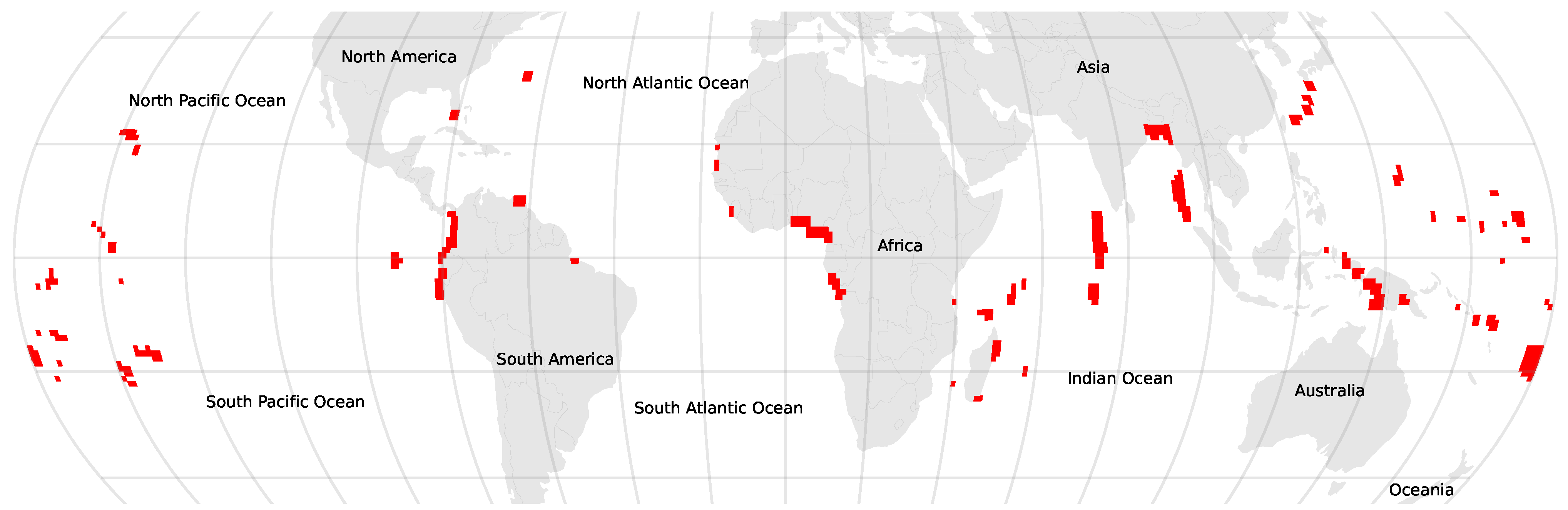
2.1. Areas to Be Mapped
Through user feedback on the GMW v2.0 maps, 204 regions were identified to be either missing or poorly mapped. As detailed by Bunting et al. [
15], the choice of 2010 for the baseline map was driven by the use of ALOS PALSAR data, coverage of which was most complete for the year 2010 [
15]. However, this resulted in Landsat-5 TM and Landsat-7 ETM+ temporal composites affected by ETM+ scan-line error artefacts, particularly in areas of high cloud cover (e.g., Niger Delta). These artefacts were, in some cases, present with the GMW v2.0 maps. Areas identified that required (re-)mapping as part of this study are shown in
Figure 1.
2.2. Mangrove Habitat Mask
Bunting et al. [
15] developed a mangrove habitat mask which was used to limit the classification of mangroves to those where mangroves can be expected to be present. For example, mangroves must generally be close to water and at or close to mean sea level. However, this mask was found to have been too tight in a number of regions (e.g., Florida, USA) and therefore caused under-classification of mangroves. Ahead of the mapping, the habitat mask was therefore revised, primarily through manually digitising regions to be added, but also intersecting the maps of [
17,
18] to ensure that all regions mapped in those products were fully located within the GMW habitat mask.
2.3. Mangrove Mapping
Bunting et al. [
15] used the most appropriate and available data (i.e., Landsat TM and ETM+ and ALOS PALSAR) for 2010 in the original mapping (v2.0). Therefore, to improve the mapping, an approach that used alternative datasets was required. In this case, Sentinel-2 imagery was used to map the areas outlined in
Figure 1. For the analysis, 100 global mangrove/non-mangrove XGBoost classifiers [
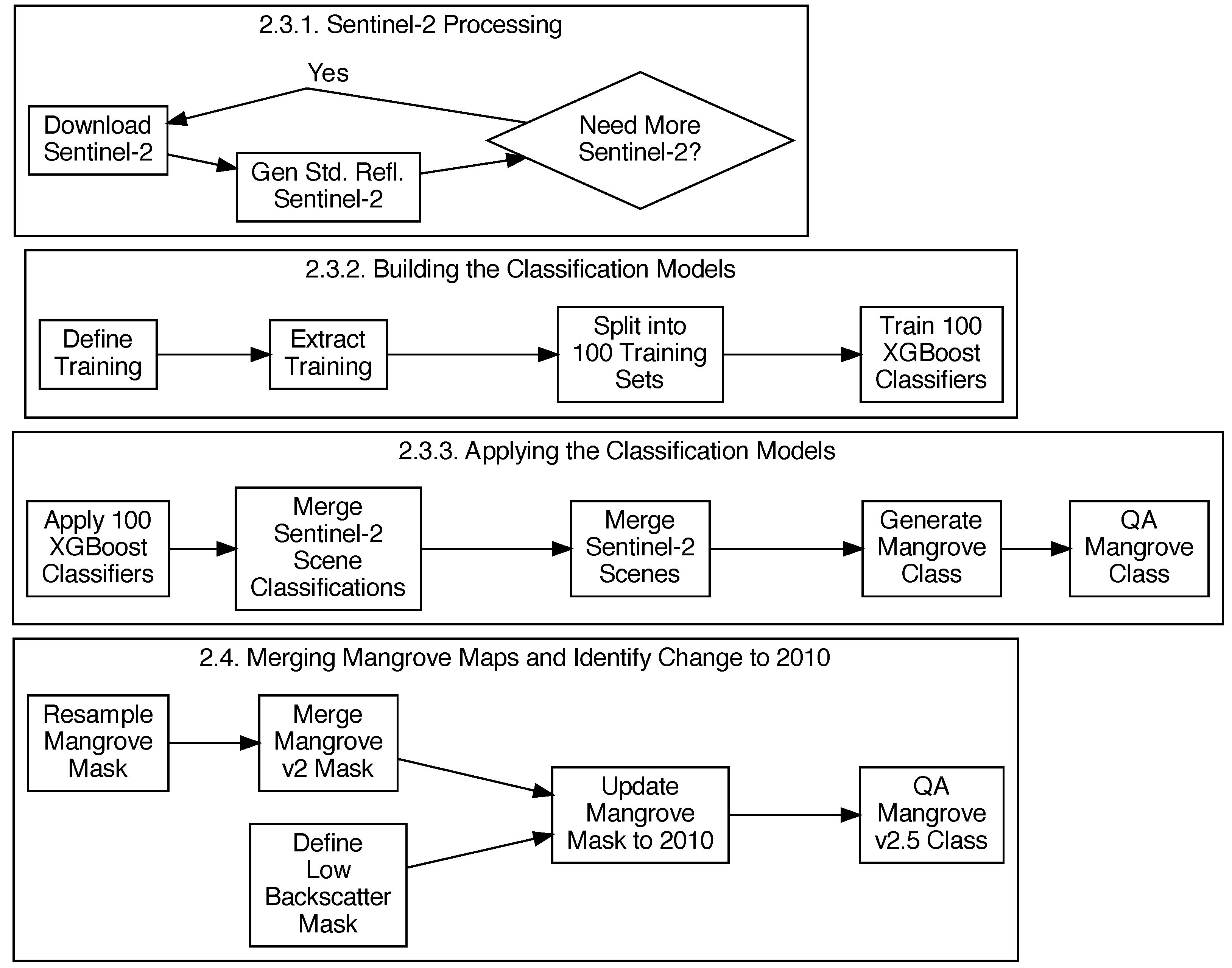
32] were trained and applied to each Sentinel-2 acquisition. To produce a single unified classification, results from all acquisitions and classifiers were merged to create a probability for each pixel to be mangroves. This probability surface was then thresholded to produce the binary map, which was subject to a manual Quality Assurance (QA) process to produce the Sentinel-2-derived maps. These were then combined with the v2.0 2010 baseline and a change detection using the 2010 ALOS PALSAR data was applied to create a revised GMW v2.5 2010 baseline. The processing stages are outlined in
Figure 2.
2.3.1. Sentinel-2 Processing
The Sentinel-2 imagery was downloaded from the Google Cloud public dataset [
33] and, for the purpose of this work, processed to a 20-m pixel resolution (i.e., the 10-m resolution Sentinel-2 image bands were resampled to 20 m using averaging) orthorectified standardised surface reflectance product. For the 383 Sentinel-2 granules identified as intersecting with the regions of interest (
Figure 1), individual acquisitions were selected for download based on cloud cover. Initially, the 10 acquisitions with the lowest cloud cover (maximum cloud cover of 20%) were identified from the entire Sentinel-2 archive (2015–2020). An iterative process was then followed where, for each granule, the scenes were downloaded and processed to produce a cloud mask. The combined cloud masks were checked to estimate whether data were available for all mangrove regions within the scene, as defined by the mangrove habitat mask. If more acquisitions were required, the thresholds for the number of acquisitions and maximum cloud cover were increased. These were increased to a maximum of 100 scenes and a maximum cloud threshold of 75%. In total, 11,262 Sentinel-2 acquisitions were downloaded and used for this analysis.
To generate a standardised reflectance product for the classifications, the ARCSI software [
34] was employed, as successfully demonstrated in past studies [
15,
26,
27,
35]. The ARCSI software uses the 6S model [
36] through the Py6S module [
37] parameterised using the image header information and an aerosol optical depth estimated from a dark object subtraction [
15]. Using the method of Shepherd and Dymond [
38], the resulting images were normalised for a sensor view angle and local topography producing a standardised reflectance product. A tropical atmosphere and maritime aerosol profile was used for all scenes.
Cloud masking was undertaken using the product of two approaches. The FMask [
39,
40] algorithm was applied using the Python-FMask implementation [
41]. The s2cloudless [
42] LightGBM classifier [
43] was also applied to each scene. The resulting s2cloudless classification was further refined using a morphological closing (with a
circular operator) followed by a morphological dilation (with a
circular operator). Finally, any cloud objects were removed if they were less than 10 pixels in size. The final cloud mask was defined as the intersection of the two masks. The cloud shadow mask was derived using the approach implemented within FMask, as described in Zhu et al. [
39].
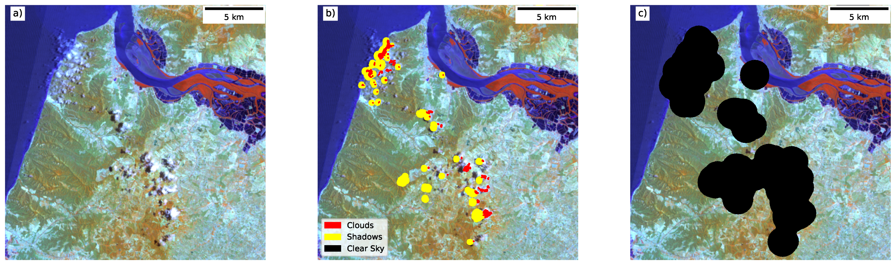
Finally, a ‘clear sky’ mask was derived for each acquisition, defining the areas of the scene to be used for further analysis. The ‘clear-sky’ mask aims to identify the larger continuous parts of the image, removing small areas between clouds. The first step buffered the cloud and cloud shadows by 30 km, clumping the remaining non-cloud regions. The non-cloud clumps with an area greater than 3000 pixels were then selected and grown to the 10-km contour of the cloud and cloud shadow pixels. An example of the ‘clear sky’ mask is shown in
Figure 3c.
2.3.2. Building the Classification Models
Classification of mangrove extent was undertaken on a scene-by-scene basis rather than through the creation of image composites (i.e., merging multiple scenes using a metric such as the greenest pixel). Image composites, whilst relevant for visualisation, often have artefacts due to prevailing environmental conditions (e.g., wet or dry season or, in the case of mangroves, tidal regimes) at the time of the acquisitions or processing errors (e.g., missed cloud or cloud shadows). These artefacts can then impact the classification result. An alternative is to classify each of the scenes independently and then merge those results to create a single map.
To derive training data for the classification, 10,284 samples were created from the existing GMW v2.0 map. These were manually checked against the Sentinel-2 imagery. For regions not already within the GMW v2.0 product training regions, these were manually defined. Non-mangrove regions were defined as regions outside of the GMW habitat product, with points sampled randomly within this region and through manual selection of regions giving a total of 52,555 sample points for training.
The resulting samples were then intersected with all 11,262 Sentinel-2 acquisitions, with each scene masked to the relevant valid clear sky area. This resulted in 4,421,644 mangrove and 9,830,388 non-mangrove pixel values to train the classifier. Given the volume of sample data available, it was decided to split the training data into 100 sets, each with 400,000 samples (200,000 for mangroves and 200,000 for non-mangroves). Those samples were then split into 3 sets for training (100,000 for each class), testing (50,000 for each class), and validating (50,000 for each class) the model.
The XGBoost [
32] binary classification algorithm was used for the analysis given its ability to use large training datasets and allow transfer learning (i.e., further training of an existing model). This method has been shown by John et al. [
35] to provide good results for the classification of land cover from Earth observation data. To optimise the hyper-parameters of the XGBoost model, a subset of 20% was selected from the training (20,000 per class) and validation (10,000 per class) samples. Bayesian optimisation was used to identify the optimal hyper-parameters for each of the 100 classifiers. The range of values for the parameters optimised is given in
Table 1. Following identification of the hyper-parameters, each of the 100 models was trained using the full dataset (i.e., 400,000 samples). The testing accuracies of the models (using the 50,000 samples per class) were between 97–99%.
2.3.3. Applying the Classification Models
To apply the 100 global XGBoost classifiers to the individual Sentinel-2 acquisitions, the models were first further trained using the local training data from the Sentinel-2 acquisition, which was limited to 25,000 samples. This allowed the global classifier to be locally optimised for the individual acquisitions. The classifiers were then applied to all the acquisitions, with this creating 112,620 classifications. To avoid incorrect classification of mangroves in areas where they would not be located (e.g., in mountainous areas), the classification was only applied within an updated version of the mangrove habitat layer of Bunting et al. [
15].
The individual classifications were then merged in two steps to create a mangrove probability for each pixel. The first step merged the 100 classifications applied to a scene to create a single probability output image for the scene. The probability was calculated as the number of times each pixel had been classified as mangroves (i.e., a value of 1 meant that all 100 classifiers classified the pixel as mangroves, while a value of 0.1 meant that only 10 classifiers classified the pixel as mangroves). The second step calculated the mean probability from all the acquisitions for each pixel, providing a single probability surface for all the areas mapped.
To derive the final binary mask of mangrove extent, a global threshold was applied to the probability surface. The threshold was identified through a sensitivity analysis using the mangrove samples based on the 0.1 increments (from 0.2 to 0.8). A mangrove mask was generated for each threshold where the mask with the best agreement with the mangrove samples used to train and test the XGBoost classifiers selected. A threshold of 0.5 provided the greatest correspondence and was therefore applied to all the regions updated using the Sentinel-2 imagery. For studies focused on specific regions, a further local optimisation could be undertaken by selecting a local threshold. However, for this study, a global threshold was applied as defining local regions would be difficult and could result in boundary artefacts within the resulting maps.
Finally, a visual assessment of the mangrove extent was undertaken where polygons identifying regions as incorrectly classified as mangroves were digitised with reference to the Sentinel-2 imagery and high-resolution Google Earth, Mapbox Satellite, and Bing maps imagery. The areas were then removed from the mangrove extent mask.
2.4. Merging Mangrove Maps and Identify Change to 2010
In addition to the new map produced from the Sentinel-2 analysis, two other mangrove maps were used to resolve issues for particular areas. For the Sundarbans, in India and Bangladesh, the mapping of Awty-Carroll et al. [
26] for the year 2010 was added to the Sentinel-2 maps to be merged with the GMW v2.0 products. The Sundarbans were significantly affected by stripping from the Landsat ETM+ data within GMW v2.0. Additionally, mangrove maps for the French overseas territories, where there was found to be a high prevalence of cloud cover that reduces the availability of useable Sentinel-2 data, generated by the French National Mangrove Observation Network [
44], were used to improve the new maps.
Following generation of the revised maps, these were merged with the existing GMW v2.0 baseline for 2010 to create the updated 2010 GMW v2.5 baseline. However, the updated areas had been mapped with data acquired over the period from 2015 to 2020 and a change detection was therefore required to backcast the map for 2010. 2010 ALOS PALSAR data were used for this and therefore the new mapping was resampled (nearest neighbour) onto the same 0.000222 degrees (∼25 m) pixel grid of the GMW v2.0 and ALOS PALSAR data layers.
As demonstrated by Thomas et al. [
3,
19,
20], mangroves produce a high backscatter response in the L-band SAR data while the majority of non-mangrove surfaces (e.g., water bodies and mudflats) have a low L-band backscatter. As a result, there is a change trajectory between mangroves and non-mangroves, which was used by Thomas et al. [
20] as the basis for a methodology for mapping mangrove change. This was applied globally to produce the GMW v2.0 change layers [
16].
For implementation, a low backscatter mask was created for 2010 and used to remove mangroves that were within the new map but not present in 2010. The mask was defined using a combination of the ALOS PALSAR 2010 layer and the Landsat-based Pekel et al. [
45] water occurrence layer generated for the period 1984–2020. The analysis was undertaken on a
degree grid, where the water occurrence layer was used to define areas that could be considered as ‘permanent’ waterbodies, defined as a water occurrence between >90 and <100. However, if no pixels were identified, then the threshold was lowered to >70. For the pixels associated with ‘permanent’ waterbodies, the 99th percentile of the SAR backscatter was calculated for both the Horizontal-Horizontal (HH) and Horizontal-Vertical (HV) polarisations. The thresholds for classifying the water extent were then calculated for both polarisations as:
If no ‘permanent’ waterbody pixels were identified, then the SAR thresholds where defined as dB in the HH and dB in the HV polarisations. To produce the low backscatter mask, the SAR backscatter was thresholded with values below those calculated above were used and the water occurrence layer had a value .
The low backscatter mask was then used to mask all the tiles, including areas which have not been remapped, updating the mangrove mask and aligning it with the ALOS PALSAR data for 2010. Finally, a Quality Assurance (QA) process was undertaken where the product was visually assessed against a variety of image sources, including high-resolution Google Earth, Mapbox Satellite and Bing Maps imagery, the Sentinel-2 data, 2010 ALOS PALSAR, and 2010 Landsat imagery data. Polygons were manually drawn for regions which should be removed from the map (i.e., not mangroves but areas that had been mapped as mangroves) or added to the map (i.e., mangroves but areas that had not been mapped as such). These QA edits were then rasterised and applied to the map producing the final GMW v2.5 layer.
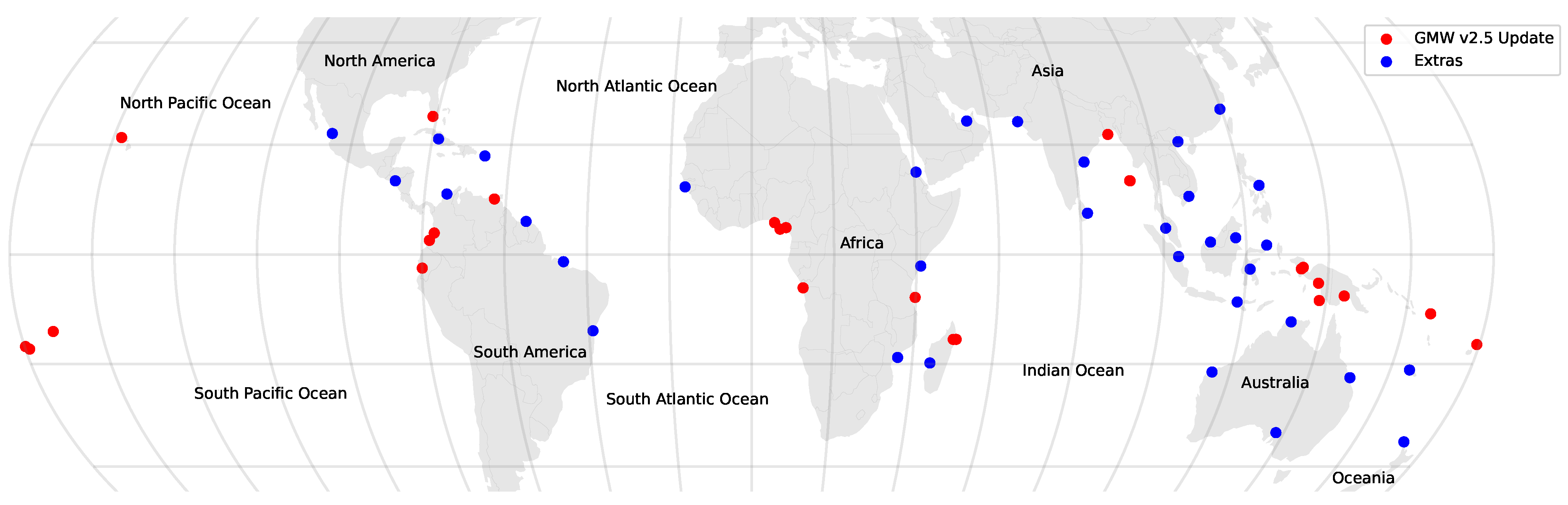
2.5. Accuracy Assessment
To assess the accuracy of the new v2.5 layer, 26 sites (
Figure 4) where new mapping had occurred were selected, representing a range of different mangrove settings, types, and extents. Additionally, a further 34 sites (
Figure 4) were distributed globally for assessing the overall product accuracy. For each site, an area of
degrees was defined and 1000 random stratified points were defined for each class (mangroves and non-mangroves). If there were less than 1000 mangrove pixels within the
degree area then all mangrove pixels were defined as points and the number of mangrove reference points was reduced. The 2000 points were then split into 200 point sets (i.e., 100 mangrove and 100 non-mangrove) where the sets were assessed in turn until the 95% confidence interval for the macro F1-score was <5%. A minimum of 3 sets (i.e., 600 points) were assessed for each site, where typically 5 sets were required (1000 points) although 10 sets were used for one site. Points were manually annotated with a reference class through a combination of high-resolution Google Earth, Mapbox Satellite and Bing Maps imagery, the Sentinel-2 and 2010 ALOS PALSAR, and Landsat imagery data. In total, 50,750 points were assessed and used for the accuracy assessment. For sites where the mapping was updated, the points were also used to assess the improvement in map accuracy achieved through this study.
3. Results
3.1. Remapped Regions Comparison
To compare the accuracy of the updated v2.5 and v2.0 GMW 2010 baselines, the reference points for the 26 sites where the baseline has been updated were intersected with both layers. Summary statistics calculated were an overall accuracy, cohen kappa, and F1 score (per-class and overall), with summaries are provided in
Table 2 and
Table 3. In addition, upper and lower confidence intervals for all metrics were calculated using bootstrapping. It was not possible to calculate metrics, such as the allocation and quantity disagreement as those metrics require a closed map where all pixels are allocated to a class such that the area of the whole region can be used to normalise. However, for this study we only have a single class of interest (i.e., mangroves).
As shown in
Table 2 and
Table 3, the estimated accuracy of mapping in regions where the quality was identified previously as poor or missed increased from 82.6% (80.1–84.9) to 95.0% (93.7–96.4). The range for the individual site accuracies also decreased from 44.7% to 12.4%, demonstrating that the quality of mapping for these areas remapped resulted in a similar quality of mapping for all regions.
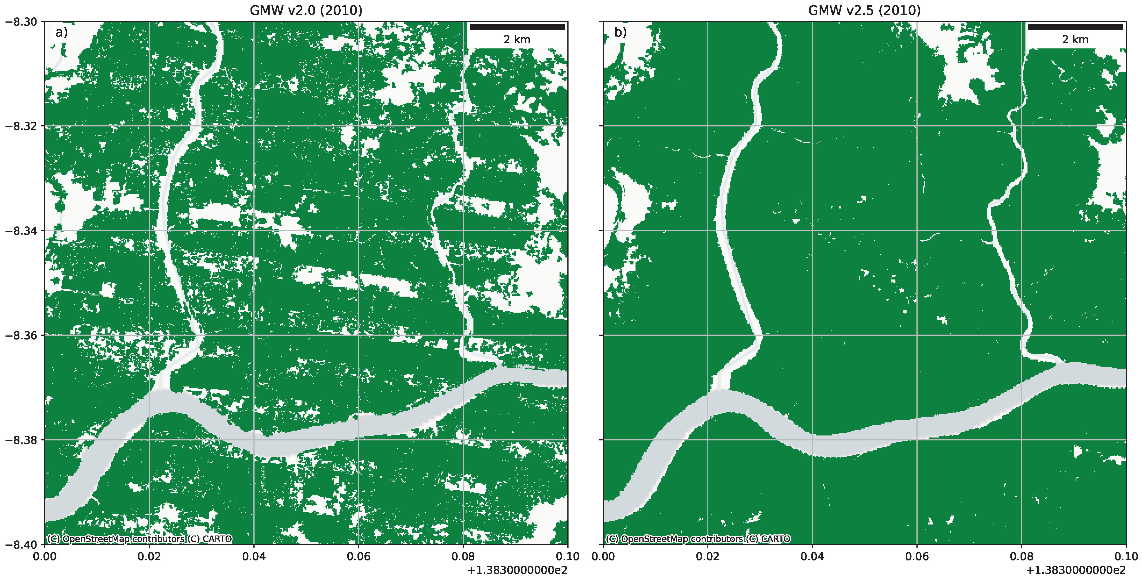
This improvement in mapping accuracy can be seen visually and is illustrated in
Figure 5,
Figure 6 and
Figure 7.
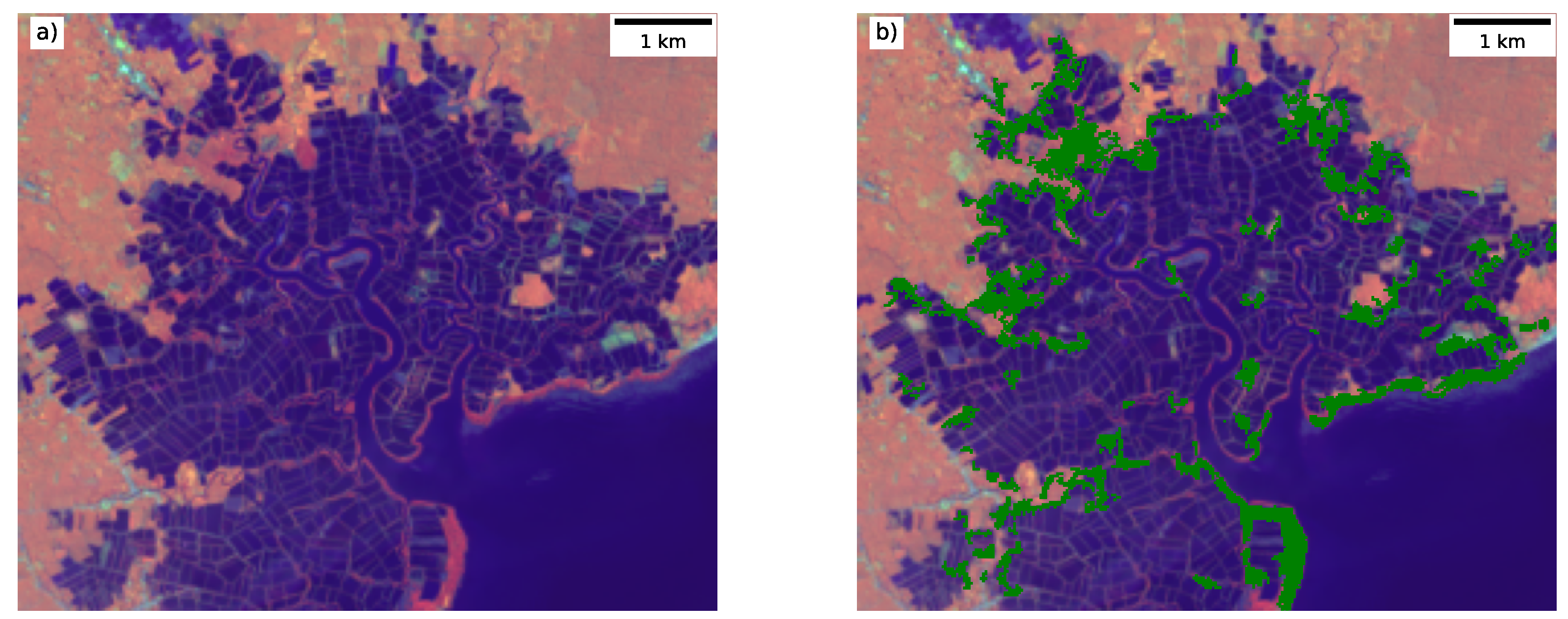
Figure 5a provides a typical example of a region that was affected by the Landsat ETM+ striping but was remapped to improve the output
Figure 5b.
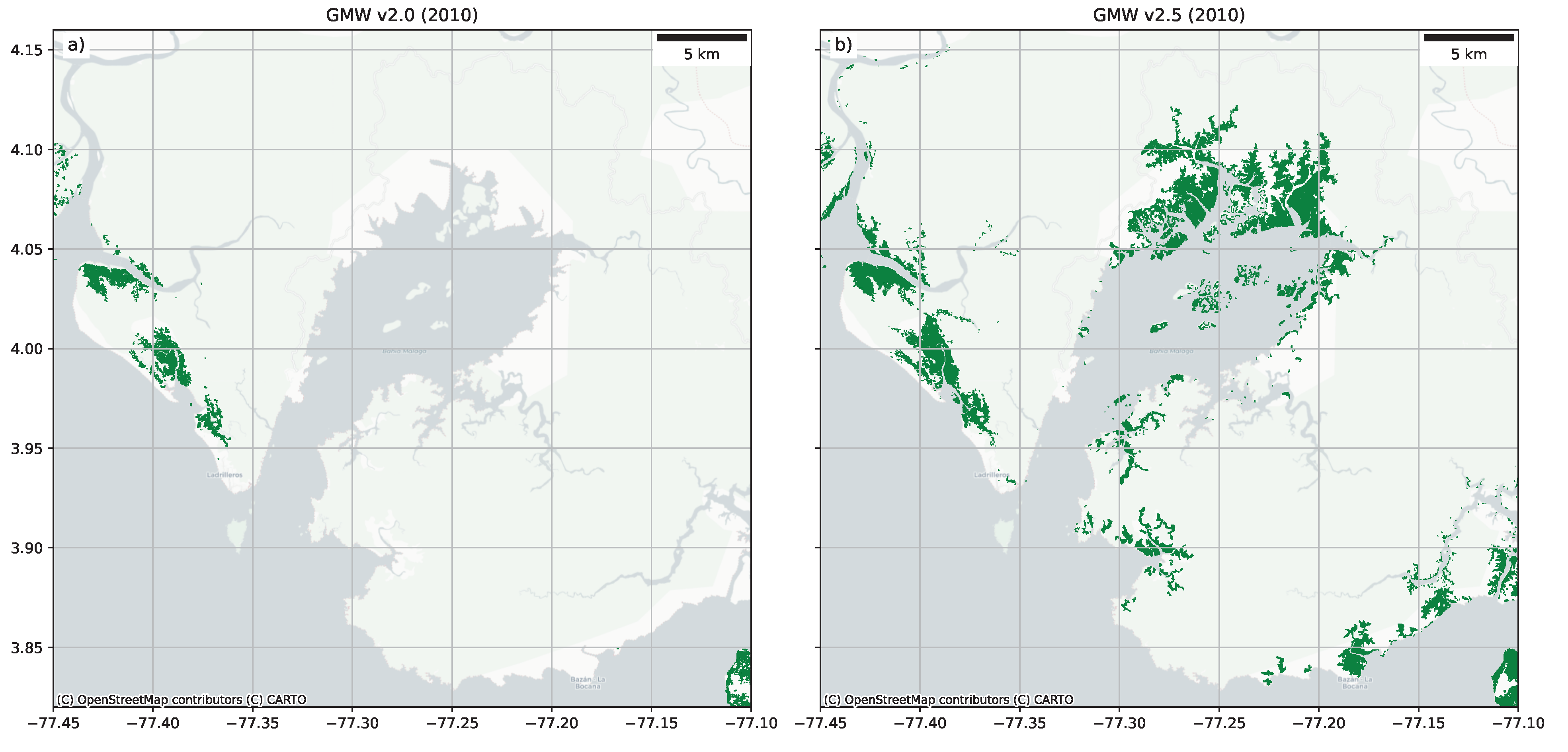
Figure 6a illustrates an area in Colombia where some areas of mangroves were missed but have now been mapped in GMW v2.5 (
Figure 6b).
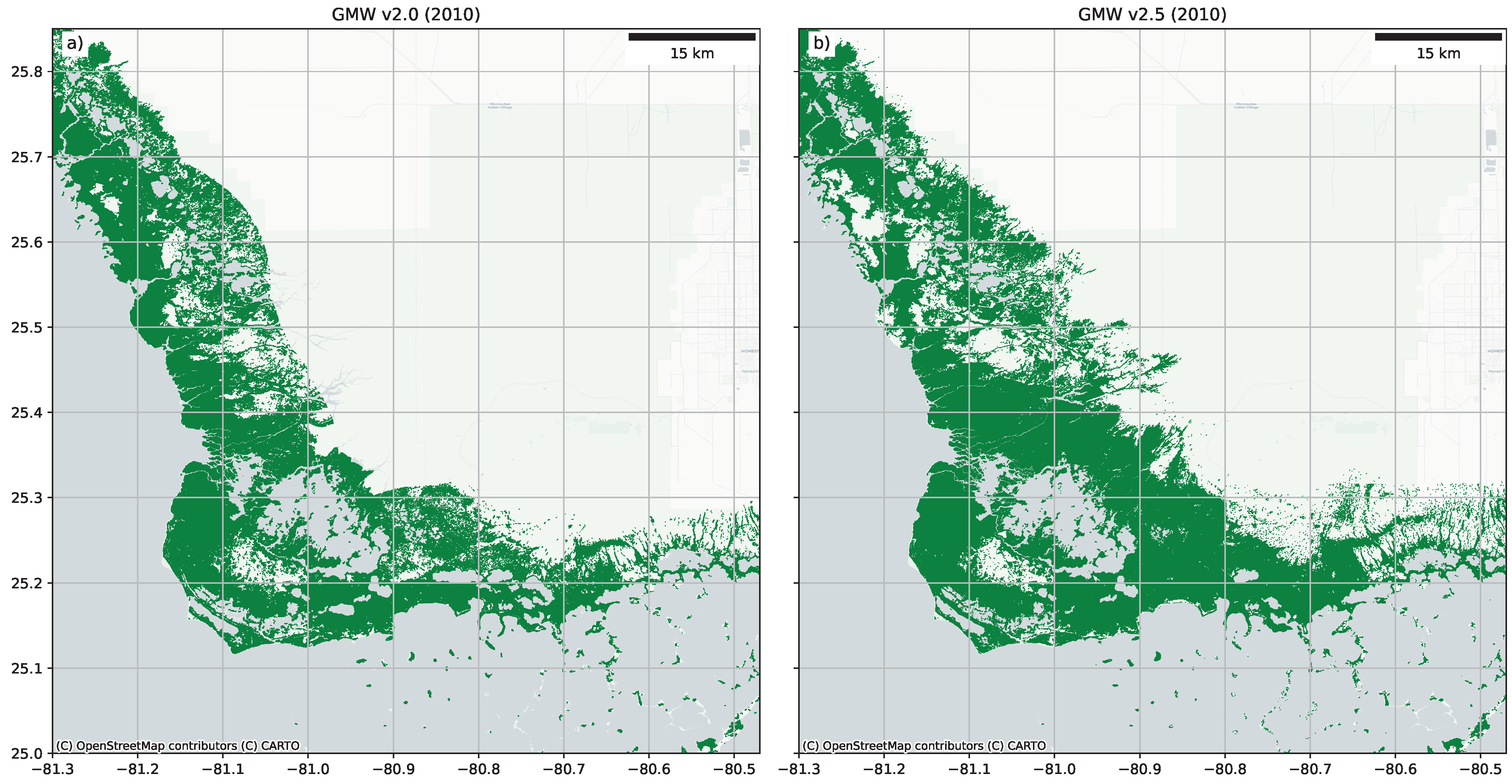
Figure 7 illustrates an example where the habitat mask was too restricted in GMW v2.0 but has been improved within GMW v2.5 by expanding the habitat mask. In terms of the accuracy statistics (
Table 3), the example shown in
Figure 6 and
Figure 7 represents a region where the accuracy will have significantly improved, while
Figure 5 resulted in only a modest statistical improvement but is visually much improved.
3.2. Overall Accuracy Assessment
Using all 60 sites, the overall accuracy statistics for the v2.5 map was calculated and presented in
Table 4. The global assessment estimated an overall accuracy of 95.1% with a 95th confidence interval (i.e., 95% likelihood that the true value is within the range) of 93.8 and 96.5%. This was similar to those published by Bunting et al. [
15] for v2.0, which estimated an overall accuracy of 94.0% with a 99th confidence interval of 93.6 and 94.5%. This is to be expected with only approximately 33% of the map having been remapped (i.e., replaced) and with only minor changes masking low backscatter pixels applied to all regions alongside the overall high estimated accuracy of the v2.0 map. However, as demonstrated in
Table 2, the local accuracy of the v2.0 map could be as low as 51% where areas were missed.
3.3. Area Statistics
The global mangrove extent mapped in v2.5 was 140,260 km
, an increase of 2660 km
(2.5%) over the v2.0 GMW map, which had a global total of 137,600 km
.
Table 5 provides a range of example countries, some with significant changes in mangrove extent between v2.5 and 2.0. A full country table of mangrove extents for v2.5 and v2.0 has been provided in
Appendix A Table A1.
Within the GMW v2.5 data, there are 121 countries with mangroves. Twelve countries, including Bermuda, were missing from the GMW v2.0, however they (and their areas) have now been added to the GMW v2.5 dataset. These were mostly small island nations where persistent cloud cover limits the acquisition of useable remote sensing data. The observed changes at a national level are variable, with 15 countries (e.g., Mozambique) having mangrove area differences of less than 1% between GMW v2.5 and v2.0, while 50 countries (e.g., Australia) had between 1–5% of change. The small changes between the two maps were attributed to the low backscatter pixel mask that was applied to all tiles. However, for countries with a small area of mangroves, these changes can be significant in percentage terms. For example, the area of mangroves mapped in Bahrain was 28% greater in the GMW v2.0.
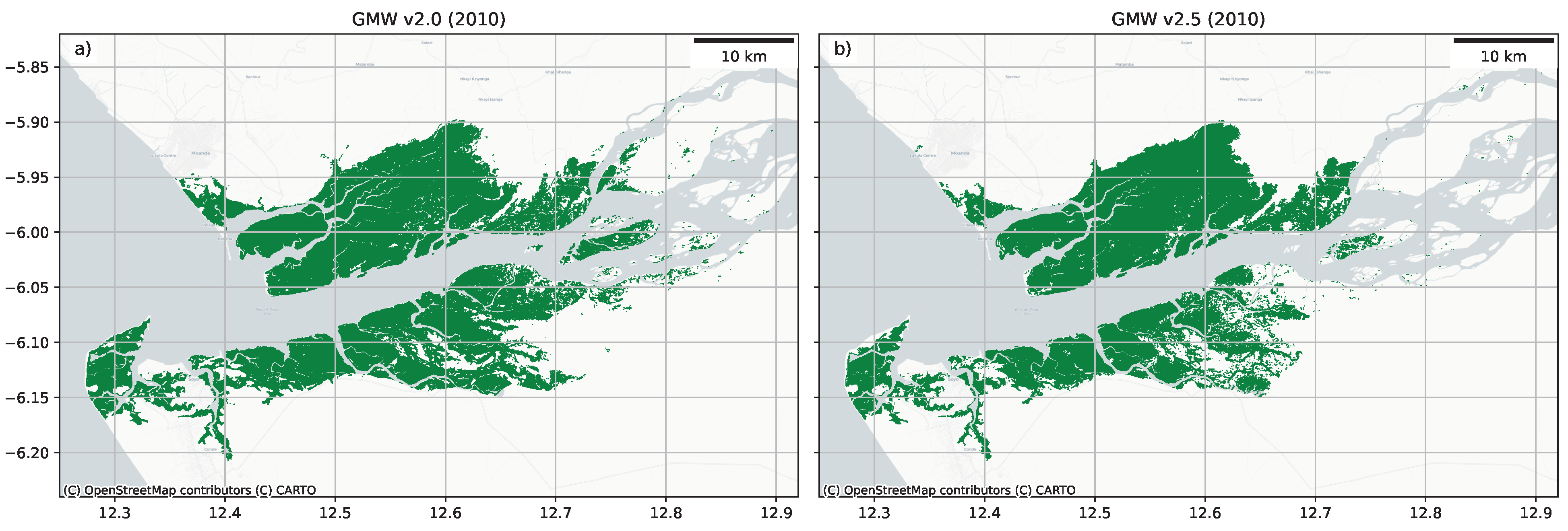
Of the remaining 44 countries, 18 had a net change between the GMW v2.5 and v2.0 between 5–10% of their mangrove area, with 11 between 10–20% and 10 between 20–50% and 5 with a net change greater than 50% of the GMW v2.0 area. Many of the countries with the largest change area were those with small mangrove extents (e.g., Bahrain or Mauritius). However, in some regions remapped with Sentinel-2, substantial areas were either removed from the GMW v2.5 map (e.g., Angola had 8377 ha of fewer mangroves;
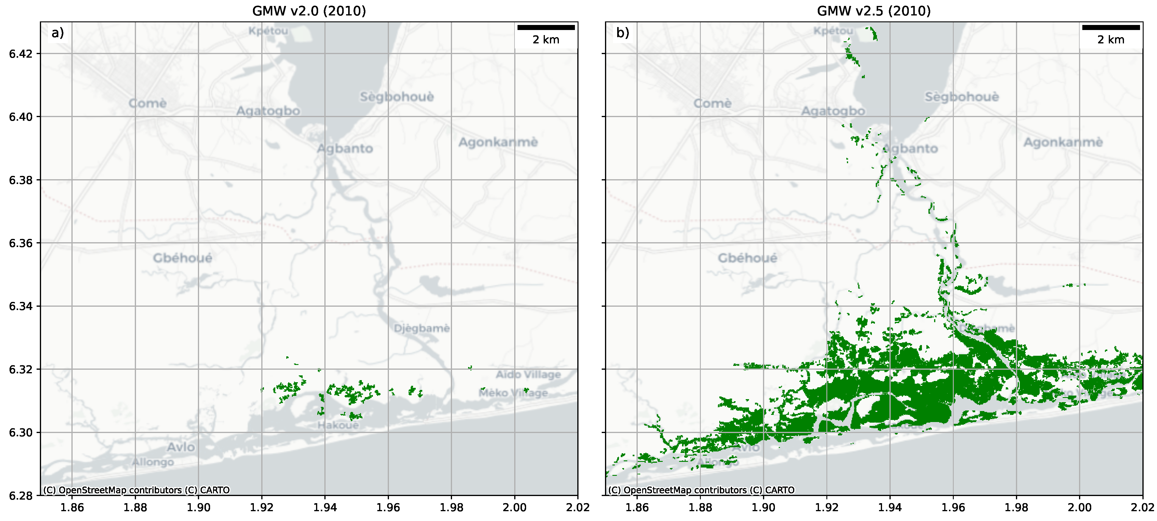
Figure 8) or were added (e.g., Benin had 3307 ha more mangroves;
Figure 9), with this improving the mangrove mask accuracy for these regions. In the GMW v2.0 map, a number of areas (e.g., Florida;
Figure 7) were omitted because of the restricted GMW habitat mask, which was used to limit areas where mangroves could be classified. Improvements in this mask along with the remapping effort has allowed new areas to be included within the GMW v2.5 map.
However, some regions were found to have a mixture of substantial omissions and commissions within the v2.0 dataset. For example, Fiji, which was remapped with Sentinel-2, had an overall net change of −2.3% between v2.0 and v2.5. However, there were also significant regions of additional mangrove within Fiji in v2.5 as a processing error in the v2.0 product caused the mangroves in the west of the island nation (i.e., –) to be missed.
The improvement in mapping through the use of the Sentinel-2 data was significant in areas of high cloud cover and particularly in regions such as French Guiana (
%), Papua New Guinea (−6.4%), Nigeria (
%), and Colombia (
%;
Figure 6). These areas had often significant striping artefacts present from the use of Landsat ETM+ data in the GMW v2.0 map (e.g.,
Figure 5).
These changes in the mapped mangrove area are not due to changes on the ground but rather to better input data (i.e., Sentinel-2) or new knowledge (e.g., improvements to the habitat mask) that have allowed us to generate a more accurate mangrove map for 2010.


 ,
, 

