
UAV Mapping of the Chlorophyll Content in a Tidal Flat Wetland Using a Combination of Spectral and Frequency Indices

Abstract
:1. Introduction
2. Materials and Methods
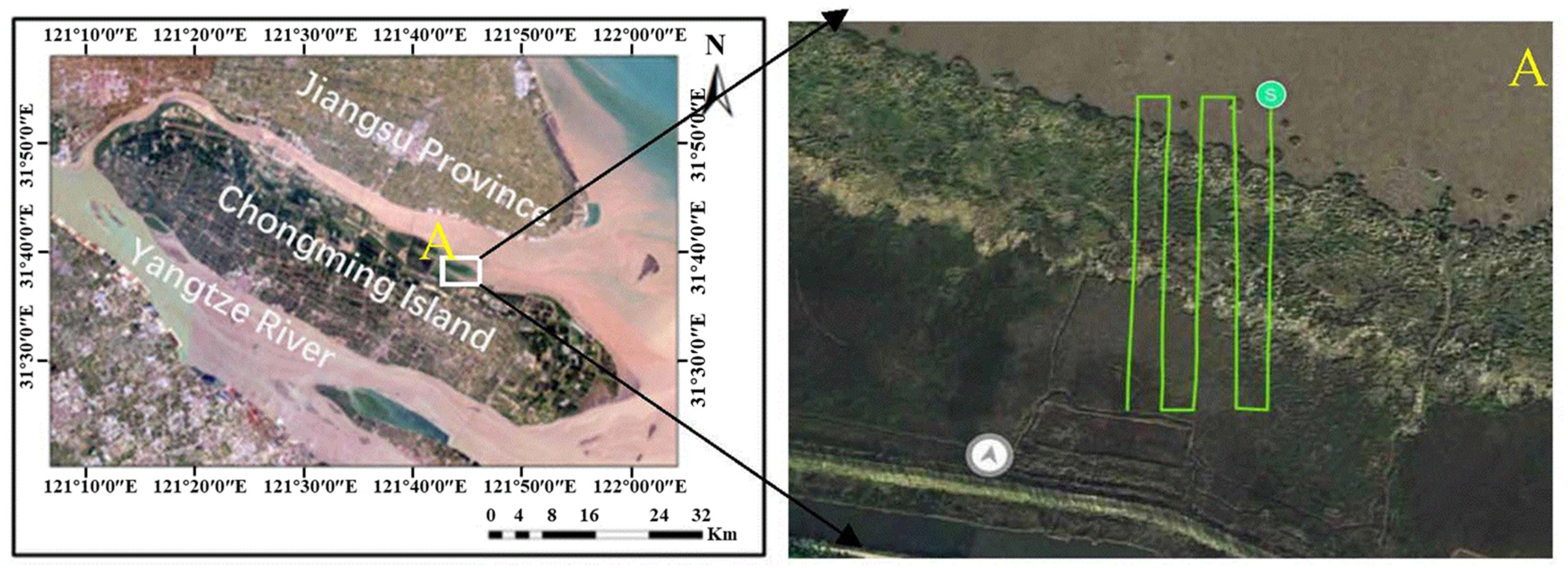
2.1. Introduction to the Study Area
2.2. Data Acquisition and Preprocessing
2.2.1. Field Experimental Design
2.2.2. Ground Data Acquisition
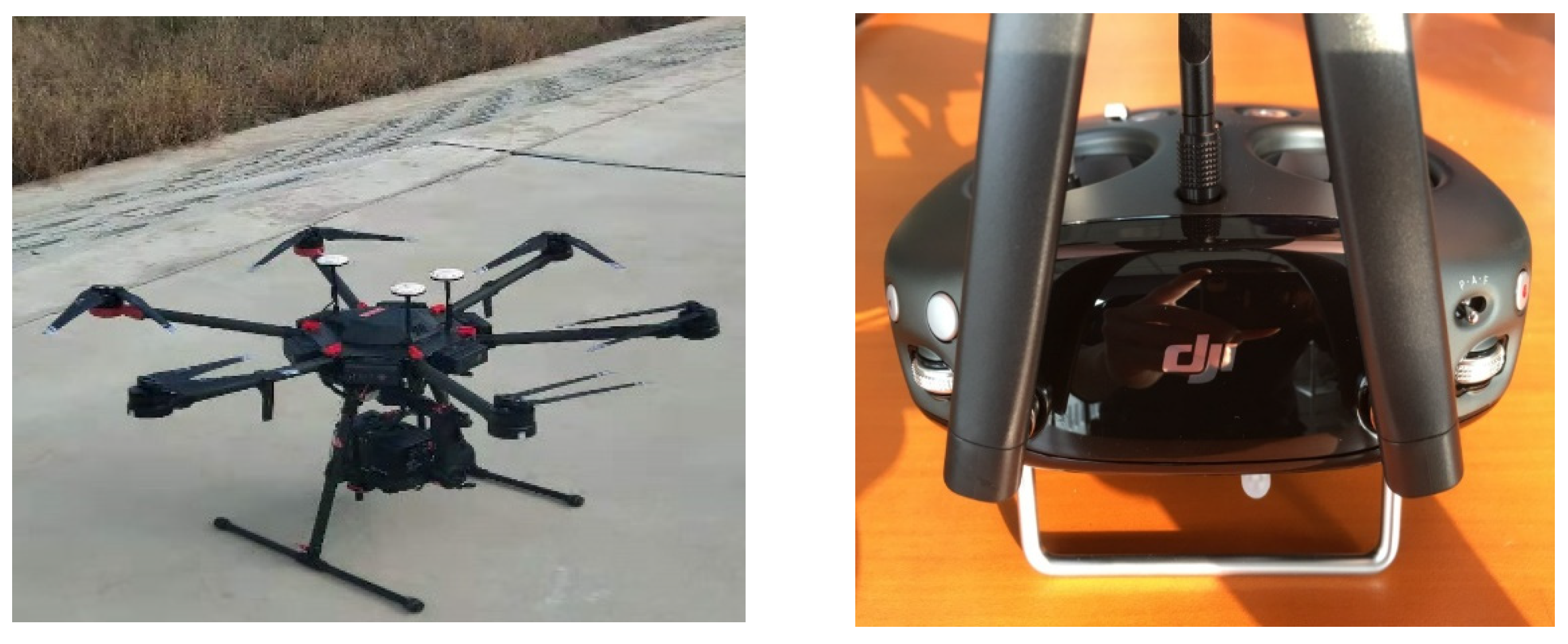
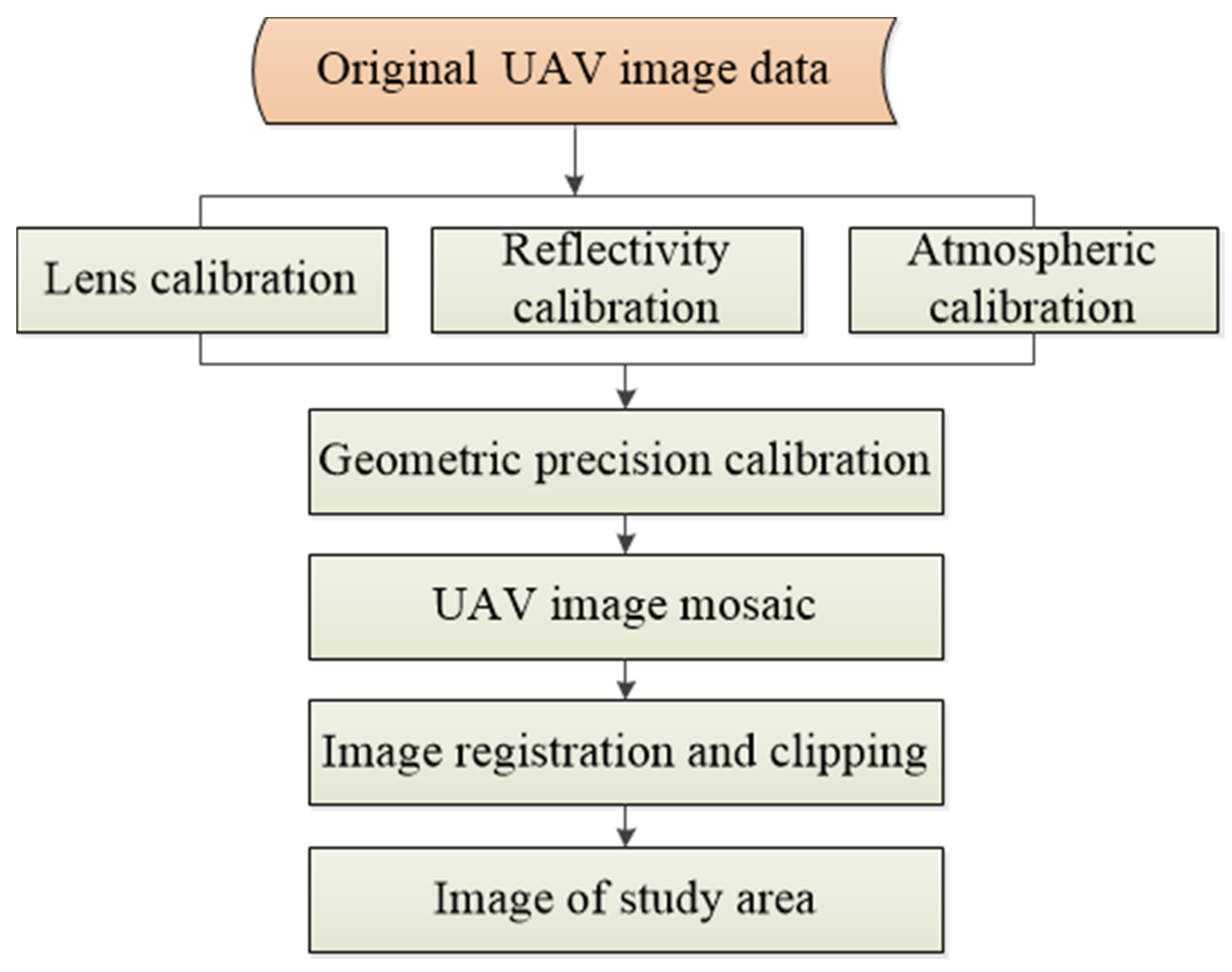
2.2.3. UAV Data Acquisition and Preprocessing
- (1)
- Introductionofthe UAV sensor parameters
- (2)
- UAV hyperspectral data acquisition and preprocessing
2.3. Harmonic Analysis
2.4. Hilbert Transformation Theory
2.5. Spectral Index and Frequency Index Calculation
2.5.1. Spectral Index Calculation
2.5.2. Frequency Index Calculation
2.6. Partial Least Squares Regression Theory
2.7. Research Technical Route
3. Results and Analysis
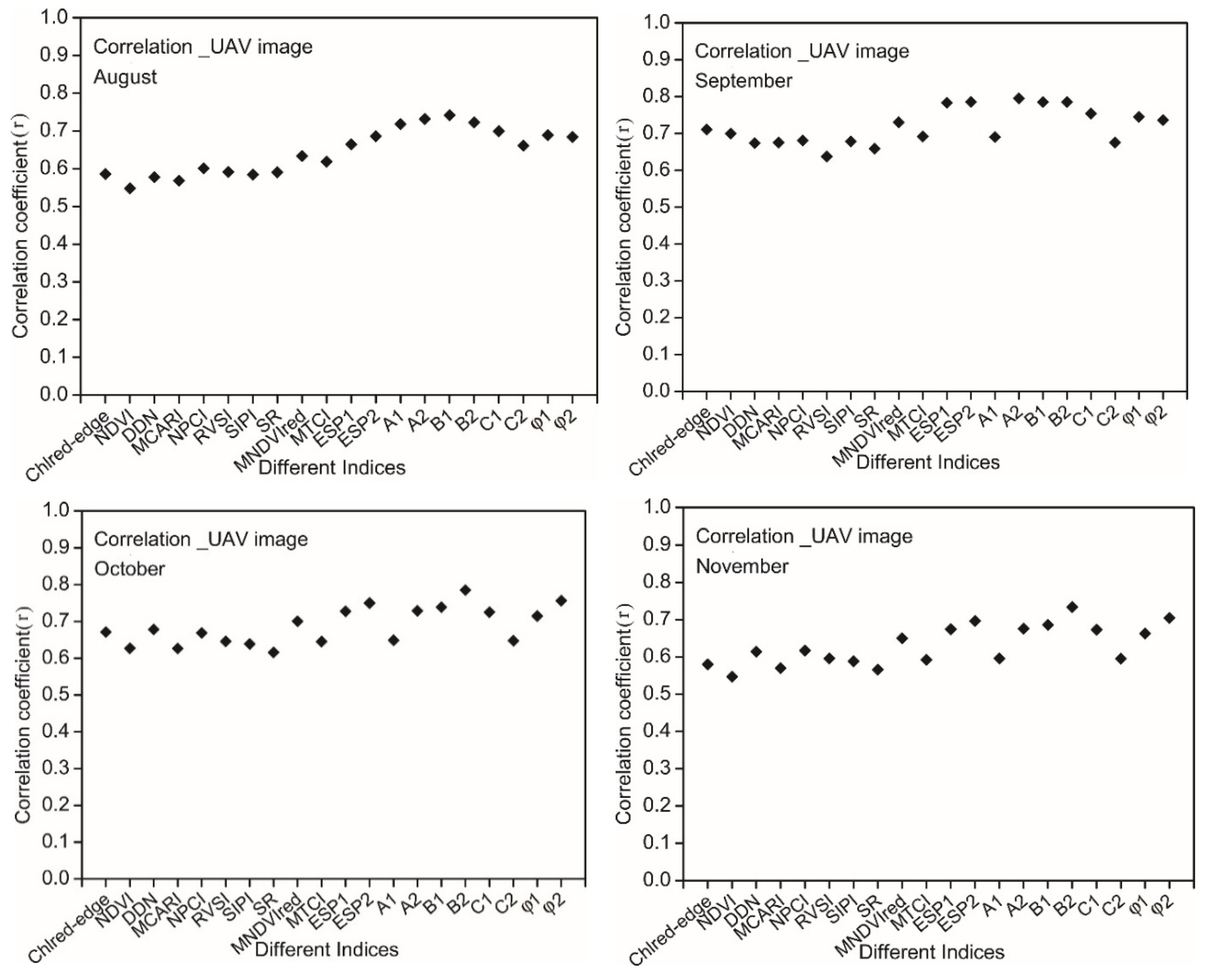
3.1. Correlation Analysis between the Indices and the Chlorophyll Content
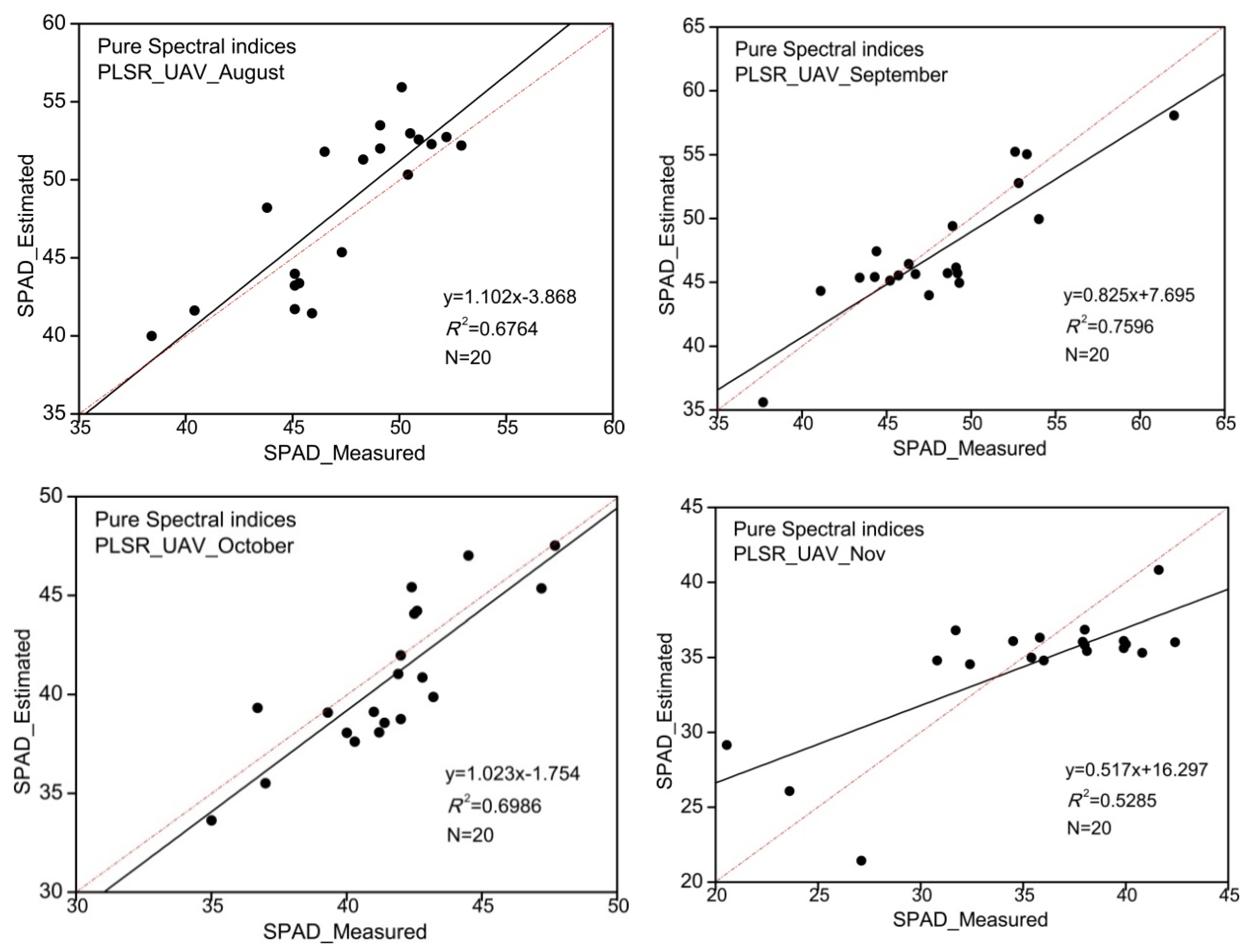
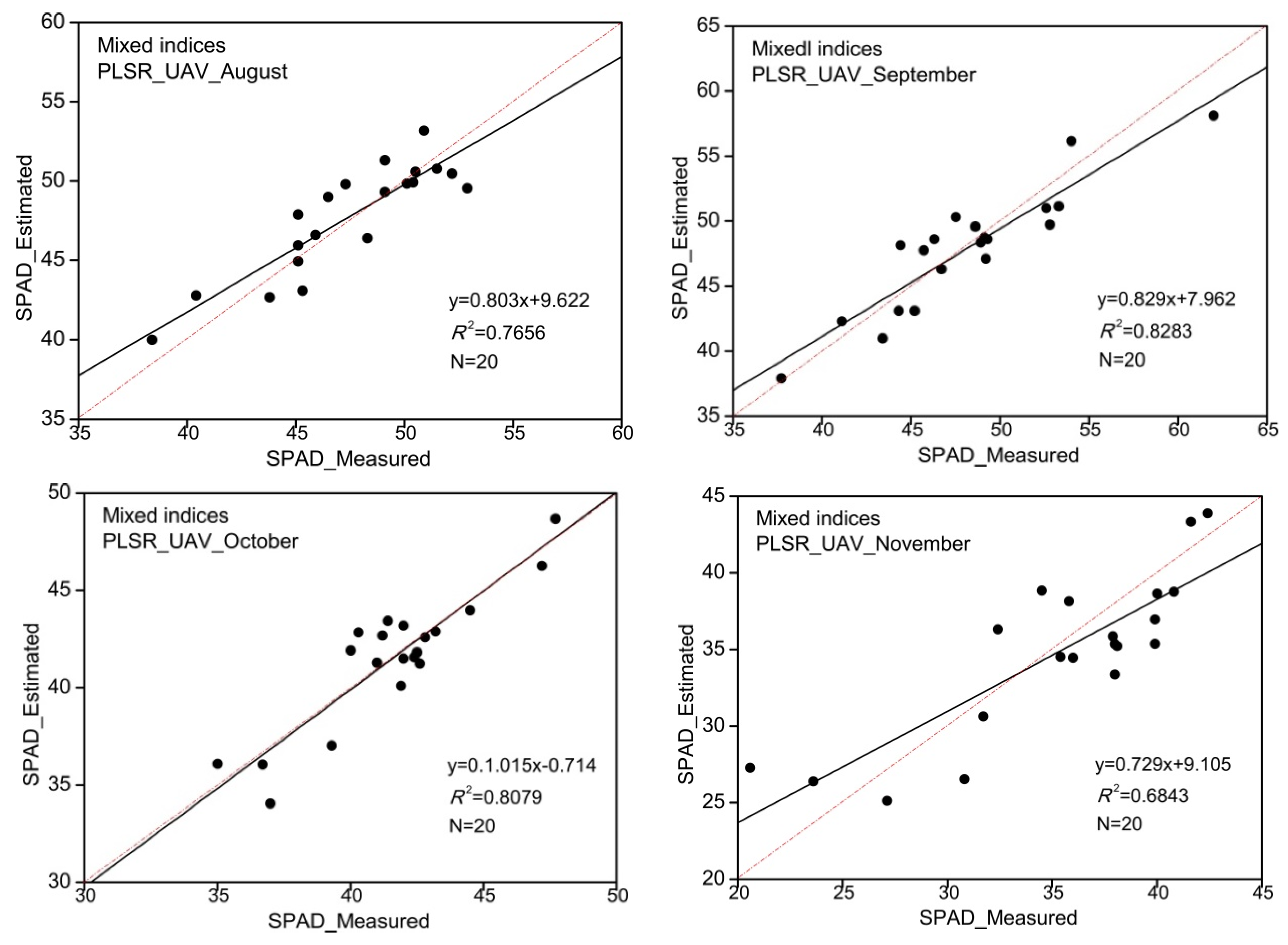
3.2. Construction of the Chlorophyll Content Estimation Model
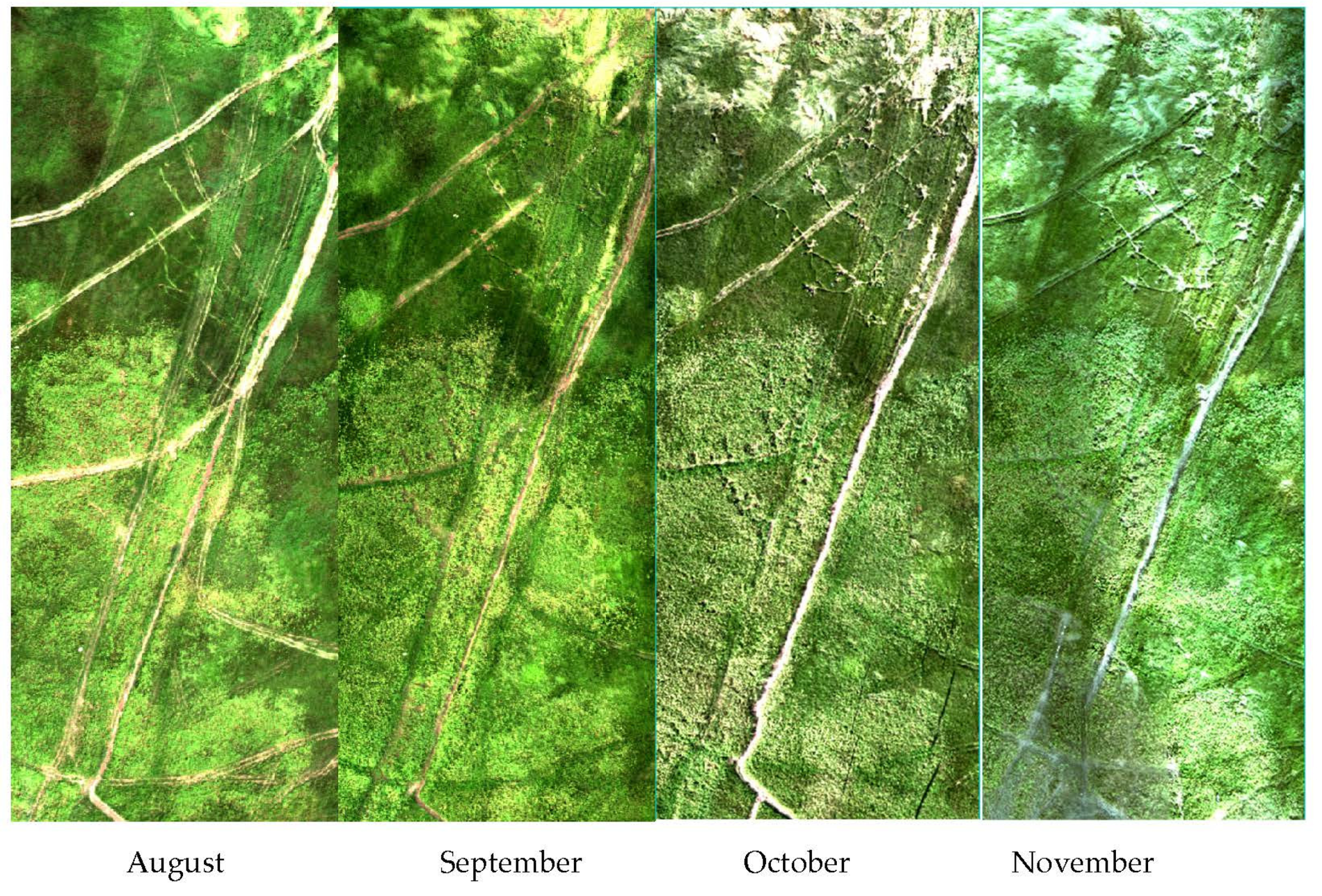
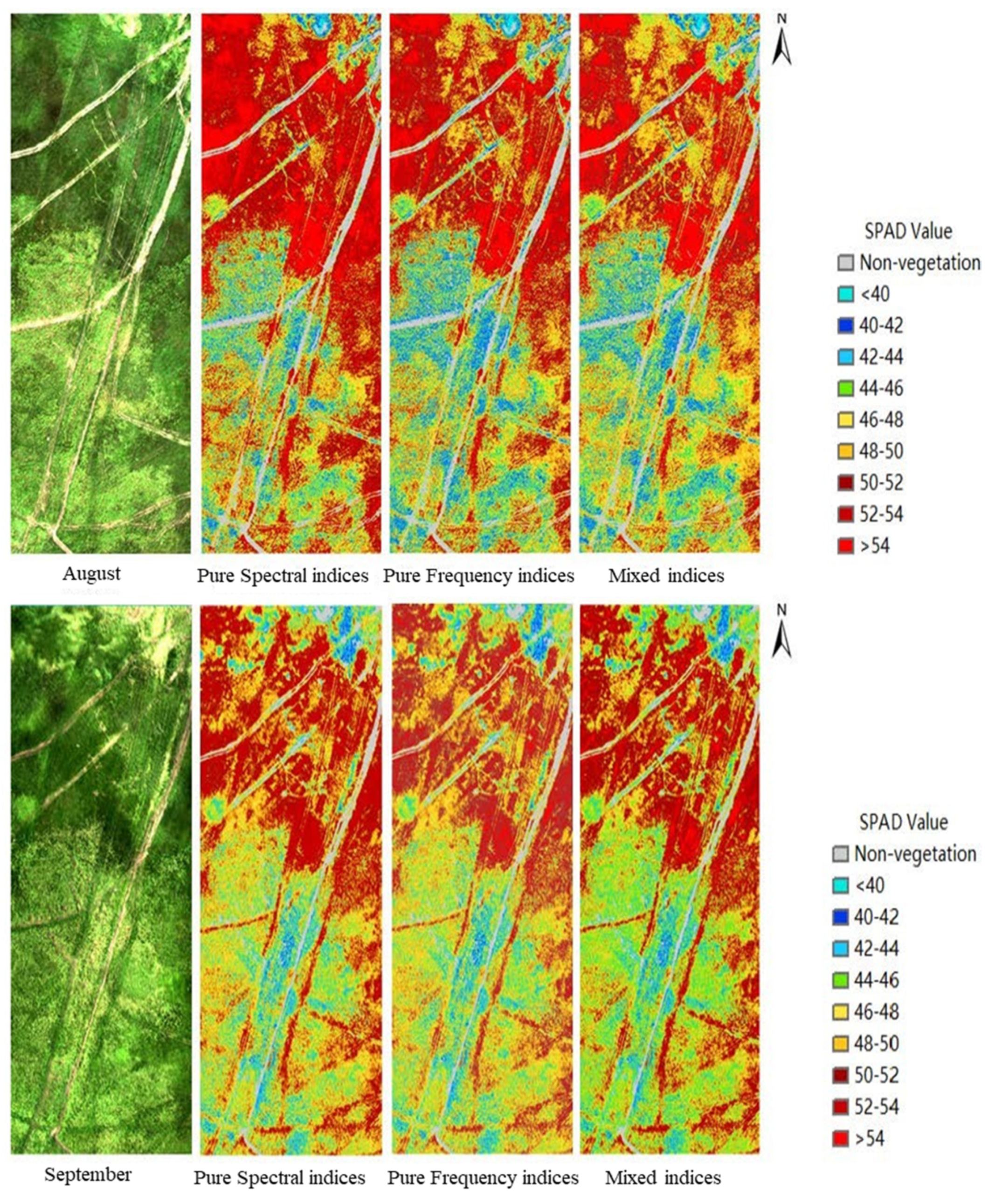
3.3. Chlorophyll Content Mapping Based on UAV Images
3.4. Verification of the Accuracy of the Chlorophyll Content Estimation Model
3.5. Analysis of SPAD Estimation in Time Series
4. Discussion
4.1. Effect of Mixed Growth on the Accuracy of Chlorophyll Content Estimation
4.2. The Influence of the Input Parameters on the Model Accuracy
5. Conclusions
Author Contributions
Funding
Institutional Review Board Statement
Informed Consent Statement
Data Availability Statement
Acknowledgments
Conflicts of Interest
References
- Rahimi, L.; Malekmohammadi, B.; Yavari, A.R. Assessing and Modeling the Impacts of Wetland Land Cover Changes on Water Provision and Habitat Quality Ecosystem Services. Nonrenewable Resour. 2020, 29, 3701–3718. [Google Scholar] [CrossRef]
- Wu, N.; Shi, R.; Zhuo, W.; Zhang, C.; Zhou, B.; Xia, Z.; Tao, Z.; Gao, W.; Tian, B. A Classification of Tidal Flat Wetland Vegetation Combining Phenological Features with Google Earth Engine. Remote Sens. 2021, 13, 443. [Google Scholar] [CrossRef]
- Moffett, K.B.; Nardin, W.; Silvestri, S.; Wang, C.; Temmerman, S. Multiple Stable States and Catastrophic Shifts in Coastal Wetlands: Progress, Challenges, and Opportunities in Validating Theory Using Remote Sensing and Other Methods. Remote Sens. 2015, 7, 10184–10226. [Google Scholar] [CrossRef] [Green Version]
- Zhuo, W.; Shi, R.; Wu, N.; Zhang, C.; Tian, B. Spectral response and the retrieval of canopy chlorophyll content under interspecific competition in wetlands—case study of wetlands in the Yangtze River Estuary. Earth Sci. Inform. 2021, 14, 1467–1486. [Google Scholar] [CrossRef]
- Ai, J.Q.; Gao, W.; Gao, Z.Q.; Shi, R.H.; Zhang, C. Phenology-based S. alterniflora mapping in coastal wetland of the Yangtze Estuary using time series of GaoFen satellite no. 1 wide field of view imagery. J. Appl. Remote Sens. 2017, 11, 026020. [Google Scholar] [CrossRef]
- Wu, N.; Shi, R.; Zhuo, W.; Zhang, C.; Tao, Z. Identification of native and invasive vegetation communities in a tidal flat wetland using gaofen-1 imagery. Wetlands 2021, 41, 46. [Google Scholar] [CrossRef]
- Han, X.; Pan, J.; Devlin, A. Remote sensing study of wetlands in the Pearl River Delta during 1995–2015 with the support vector machine method. Front. Earth Sci. 2017, 12, 521–531. [Google Scholar] [CrossRef]
- Ren, G.-B.; Wang, J.-J.; Wang, A.-D.; Wang, J.-B.; Zhu, Y.-L.; Wu, P.-Q.; Ma, Y.; Zhang, J. Monitoring the Invasion of Smooth Cordgrass Spartina alterniflora within the Modern Yellow River Delta Using Remote Sensing. J. Coast. Res. 2019, 90, 135–145. [Google Scholar] [CrossRef]
- Sun, L.; Shao, D.; Xie, T.; Gao, W.; Ma, X.; Ning, Z.; Cui, B. How Does Spartina alterniflora Invade in Salt Marsh in Relation to Tidal Channel Networks? Patterns and Processes. Remote Sens. 2020, 12, 2983. [Google Scholar] [CrossRef]
- Ma, H.; Liu, Y.; Ren, Y.; Wang, D.; Yu, L.; Yu, J. Improved CNN Classification Method for Groups of Buildings Damaged by Earthquake, Based on High Resolution Remote Sensing Images. Remote Sens. 2020, 12, 260. [Google Scholar] [CrossRef] [Green Version]
- Wu, W.; Wang, W.; Meadows, M.E.; Yao, X.; Peng, W. Cloud-based typhoon-derived paddy rice flooding and lodging detection using multi-temporal Sentinel-1&2. Front. Earth Sci. 2019, 13, 682–694. [Google Scholar] [CrossRef]
- Jin, J.; Hao, M. Registration of UAV Images Using Improved Structural Shape Similarity Based on Mathematical Morphology and Phase Congruency. IEEE J. Sel. Top. Appl. Earth Obs. Remote Sens. 2020, 13, 1503–1514. [Google Scholar] [CrossRef]
- Duan, B.; Liu, Y.; Gong, Y.; Peng, Y.; Wu, X.; Zhu, R.; Fang, S. Remote estimation of rice LAI based on Fourier spectrum texture from UAV image. Plant Methods 2019, 15, 124. [Google Scholar] [CrossRef] [Green Version]
- Al-Ali, Z.M.; Abdullah, M.; Asadalla, N.B.; Gholoum, M. A comparative study of remote sensing classification methods for monitoring and assessing desert vegetation using a UAV-based multispectral sensor. Environ. Monit. Assess. 2020, 192, 389. [Google Scholar] [CrossRef]
- Fenger-Nielsen, R.; Hollesen, J.; Matthiesen, H.; Andersen, E.S.; Westergaard-Nielsen, A.; Harmsen, H.; Michelsen, A.; Elberling, B. Footprints from the past: The influence of past human activities on vegetation and soil across five archaeological sites in Greenland. Sci. Total Environ. 2018, 654, 895–905. [Google Scholar] [CrossRef] [PubMed]
- Kattenborn, T.; Eichel, J.; Wiser, S.; Burrows, L.; Fassnacht, F.E.; Schmidtlein, S. Convolutional Neural Networks accurately predict cover fractions of plant species and communities in Unmanned Aerial Vehicle imagery. Remote. Sens. Ecol. Conserv. 2020, 6, 472–486. [Google Scholar] [CrossRef] [Green Version]
- Mazzia, V.; Comba, L.; Khaliq, A.; Chiaberge, M.; Gay, P. UAV and Machine Learning Based Refinement of a Satellite-Driven Vegetation Index for Precision Agriculture. Sensors 2020, 20, 2530. [Google Scholar] [CrossRef]
- Li, C.; Ma, C.; Cui, Y.; Lu, G.; Wei, F. UAV Hyperspectral Remote Sensing Estimation of Soybean Yield Based on Physiological and Ecological Parameter and Meteorological Factor in China. J. Indian Soc. Remote Sens. 2020, 49, 873–886. [Google Scholar] [CrossRef]
- Xu, J.-X.; Ma, J.; Tang, Y.-N.; Wu, W.-X.; Shao, J.-H.; Wu, W.-B.; Wei, S.-Y.; Liu, Y.-F.; Wang, Y.-C.; Guo, H.-Q. Estimation of Sugarcane Yield Using a Machine Learning Approach Based on UAV-LiDAR Data. Remote Sens. 2020, 12, 2823. [Google Scholar] [CrossRef]
- Mink, R.; Linn, A.I.; Santel, H.; Gerhards, R. Sensor-based evaluation of maize (Zea mays) and weed response to post-emergence herbicide applications of Isoxaflutole and Cyprosulfamide applied as crop seed treatment or herbicide mixing partner. Pest Manag. Sci. 2019, 76, 1856–1865. [Google Scholar] [CrossRef]
- Banerjee, B.; Raval, S.; Cullen, P.J. UAV-hyperspectral imaging of spectrally complex environments. Int. J. Remote Sens. 2020, 41, 4136–4159. [Google Scholar] [CrossRef]
- Zhang, X.; Han, L.; Dong, Y.; Shi, Y.; Huang, W.; Han, L.; González-Moreno, P.; Ma, H.; Ye, H.; Sobeih, T. A Deep Learning-Based Approach for Automated Yellow Rust Disease Detection from High-Resolution Hyperspectral UAV Images. Remote Sens. 2019, 11, 1554. [Google Scholar] [CrossRef] [Green Version]
- Zhu, X.; Meng, L.; Zhang, Y.; Weng, Q.; Morris, J. Tidal and Meteorological Influences on the Growth of Invasive Spartina alterniflora: Evidence from UAV Remote Sensing. Remote Sens. 2019, 11, 1208. [Google Scholar] [CrossRef] [Green Version]
- Shukla, A.; Jain, K. Automatic extraction of urban land information from unmanned aerial vehicle (UAV) data. Earth Sci. Inform. 2020, 13, 1225–1236. [Google Scholar] [CrossRef]
- Kolanuvada, S.R.; Ilango, K.K. Automatic Extraction of Tree Crown for the Estimation of Biomass from UAV Imagery Using Neural Networks. J. Indian Soc. Remote Sens. 2020, 49, 651–658. [Google Scholar] [CrossRef]
- Wu, C.; Niu, Z.; Tang, Q.; Huang, W. Estimating chlorophyll content from hyperspectral vegetation indices: Modeling and validation. Agric. For. Meteorol. 2008, 148, 1241. [Google Scholar] [CrossRef]
- Main, R.; Cho, M.A.; Mathieu, R.; O’Kennedy, M.M.; Ramoelo, A.; Koch, S. An investigation into robust spectral indices for leaf chlorophyll estimation. ISPRS J. Photogramm. Remote Sens. 2011, 66, 751–761. [Google Scholar] [CrossRef]
- Liu, P.; Shi, R.; Zhang, C.; Zeng, Y.; Wang, J.; Tao, Z.; Gao, W. Integrating multiple vegetation indices via an artificial neural network model for estimating the leaf chlorophyll content of S. alterniflora under interspecies competition. Environ. Monit. Assess. 2017, 189, 596. [Google Scholar] [CrossRef]
- Zhuo, W.; Shi, R.; Zhang, C.; Gao, W.; Liu, P.; Wu, N.; Tao, Z. A novel method for leaf chlorophyll retrieval based on harmonic analysis: A case study on Spartina alterniflora. Earth Sci. Inform. 2020, 13, 747–762. [Google Scholar] [CrossRef]
- Cloutis, E.A. Review Article Hyperspectral geological remote sensing: Evaluation of analytical techniques. Int. J. Remote Sens. 1996, 17, 2215–2242. [Google Scholar] [CrossRef]
- Jakubauskas, M.E.; Legates, D.R.; Kastens, J.H. Crop identification using harmonic analysis of time-series AVHRR NDVI data. Comput. Electron. Agric. 2002, 37, 127–139. [Google Scholar] [CrossRef]
- Huang, N.E.; Shen, Z.; Long, S.R.; Wu, M.C.; Shih, H.H.; Zheng, Q.; Yen, N.-C.; Tung, C.C.; Liu, H.H. The empirical mode decomposition and the Hilbert spectrum for nonlinear and non-stationary time series analysis. Proc. R. Soc. Lond. A 1998, 454, 903–995. [Google Scholar] [CrossRef]
- Gitelson, A.A.; Keydan, G.P.; Merzlyak, M.N. Three-band model for noninvasive estimation of chlorophyll, carotenoids, and anthocyanin contents in higher plant leaves. Geophys. Res. Lett. 2006, 33, L11402. [Google Scholar] [CrossRef] [Green Version]
- Defries, R.S.; Townshend, J.R.G. NDVI-derived land cover classifications at a global scale. Int. J. Remote Sens. 1994, 15, 3567–3586. [Google Scholar] [CrossRef]
- le Maire, G.; Franois, C.; Soudani, K.; Berveiller, D.; Pontailler, J.-Y.; Bréda, N.; Genet, H.; Davi, H.; Dufrêne, E. Calibration and validation of hyperspectral indices for the estimation of broadleaved forest leaf chlorophyll content, leaf mass per area, leaf area index and leaf canopy biomass. Remote Sens. Environ. 2008, 112, 3846–3864. [Google Scholar] [CrossRef]
- Viswanath, S.K.; Tripathi, N.K.; Salin, K.R. Mapping of Marine Chl-a and Suspended Solid Concentration Using OCM-2 Sensor. J. Indian Soc. Remote Sens. 2018, 46, 675–685. [Google Scholar] [CrossRef]
- Peñuelas, J.; Gamon, J.A.; Fredeen, A.L.; Merino, J.; Field, C.B. Reflectance indices associated with physiological changes in nitrogen- and water-limited sunflower leaves. Remote Sens. Environ. 1994, 48, 135–146. [Google Scholar] [CrossRef]
- Martin, M.E.; Newman, S.D.; Aber, J.D.; Congalton, R.G. Determining Forest Species Composition Using High Spectral Resolution Remote Sensing Data. Remote Sens. Environ. 1998, 65, 249–254. [Google Scholar] [CrossRef]
- Filella, I.; Porcar-Castell, A.; Munné-Bosch, S.; Bäck, J.; Garbulsky, M.F.; Peñuelas, J. PRI assessment of long-term changes in carotenoids/chlorophyll ratio and short-term changes in de-epoxidation state of the xanthophyll cycle. Int. J. Remote Sens. 2009, 30, 4443–4455. [Google Scholar] [CrossRef]
- Alves, E.G.; Harley, P.; Gonçalves, J.F.C.; da Silva Moura, C.E.; Jardine, K. Effects of light and temperature on isoprene emission at different leaf developmental stages of Eschweilera coriacea in central Amazon. Acta Amaz. 2013, 44, 9–18. [Google Scholar] [CrossRef]
- Jürgens, C. The modified normalized difference vegetation index (mNDVI) a new index to determine frost damages in agriculture based on Landsat TM data. Int. J. Remote Sens. 1997, 18, 3583–3594. [Google Scholar] [CrossRef]
- Nagler, P.L. Leaf area index and normalized difference vegetation index as predictors of canopy characteristics and light interception by riparian species on the Lower Colorado River. Agric. For. Meteorol. 2004, 125, 1–17. [Google Scholar] [CrossRef]
- Mishra, P.; Nikzad-Langerodi, R. Partial least square regression versus domain invariant partial least square regression with application to near-infrared spectroscopy of fresh fruit. Infrared Phys. Technol. 2020, 111, 103547. [Google Scholar] [CrossRef]


| Spectral Range | Frame Pixels | Spectral Resolution | Sensor | Lens Parameter | Carrying Platform |
|---|---|---|---|---|---|
| 400–1000 nm | 1392 × 1040 | 3.5 nm ± 0.5 nm | CCD ICX285 | 23 mm | Load > 3 kg |
| Spectral Index Definition | Abbreviation | Calculation | Ref. |
|---|---|---|---|
| Chlorophyll Red-edge Index (Chlred-edge) | Chlred-edge | (R780/R705) − 1 | [33] |
| Normalized Difference Vegetation Index | NDVI | (R800 − R670)/(R800 + R670) | [34] |
| Double Difference Index (DDN) | DDN | 2 R710 − R660 − R760 | [35] |
| Modified Chlorophyll Absorption in Reflectance Index (MCARI) | MCARI | [(R701 − R671) − 0.2(R701 − R549)]/(R701/R671) | [36] |
| Normalized Pigment Chlorophyll Index | NPCI | (R680 − R430)/(R680 + R430) | [37] |
| Red edge Vegetation Stress Index (RVSI) | RVSI | (R712 + R752)/2 − R732 | [38] |
| Structure-insensitive Pigment Index (SIPI) | SIPI | (R800 − R445)/(R800 − R680) | [39] |
| Simple Ratio (SR) | SR | R800/R670 | [40] |
| Modified Red-edge Normalized Difference Vegetation Index | MNDVIred | (R750 − R705)/(R750 + R705 − R445) | [41] |
| Meris Terrestrial Chlorophyll Index | MTCI | (R754 − R709)/(R709 − R681) | [42] |
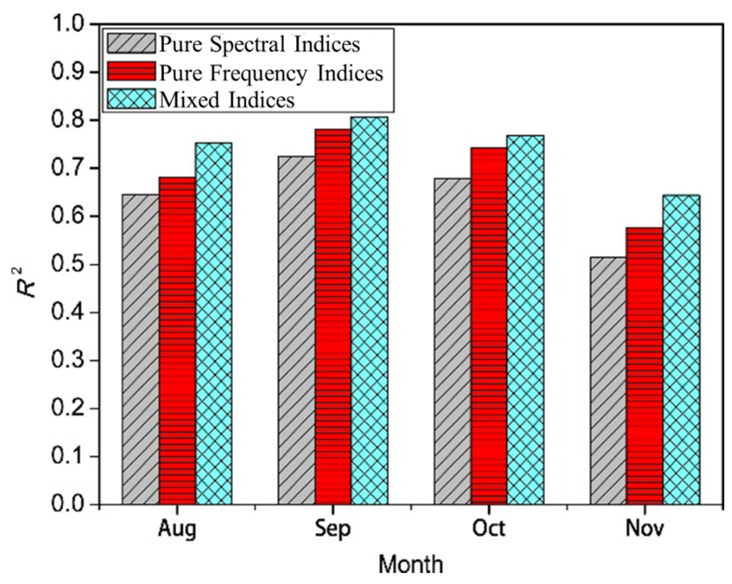
| Index | August | September | October | November | ||||
|---|---|---|---|---|---|---|---|---|
| R2 | RMSE | R2 | RMSE | R2 | RMSE | R2 | RMSE | |
| Pure Spectral Indices | 0.6459 | 2.9618 | 0.7246 | 2.5768 | 0.6784 | 2.3675 | 0.5143 | 4.4254 |
| Pure Spectral Indices | 0.6817 | 2.6835 | 0.7817 | 2.3876 | 0.7421 | 1.9879 | 0.5767 | 3.7585 |
| Mixed Indices | 0.7525 | 2.1757 | 0.8073 | 2.0943 | 0.7684 | 1.5685 | 0.6438 | 3.1548 |
Publisher’s Note: MDPI stays neutral with regard to jurisdictional claims in published maps and institutional affiliations. |
© 2022 by the authors. Licensee MDPI, Basel, Switzerland. This article is an open access article distributed under the terms and conditions of the Creative Commons Attribution (CC BY) license (https://creativecommons.org/licenses/by/4.0/).
Share and Cite
Zhuo, W.; Wu, N.; Shi, R.; Wang, Z. UAV Mapping of the Chlorophyll Content in a Tidal Flat Wetland Using a Combination of Spectral and Frequency Indices. Remote Sens. 2022, 14, 827. https://doi.org/10.3390/rs14040827
Zhuo W, Wu N, Shi R, Wang Z. UAV Mapping of the Chlorophyll Content in a Tidal Flat Wetland Using a Combination of Spectral and Frequency Indices. Remote Sensing. 2022; 14(4):827. https://doi.org/10.3390/rs14040827
Chicago/Turabian StyleZhuo, Wei, Nan Wu, Runhe Shi, and Zuo Wang. 2022. "UAV Mapping of the Chlorophyll Content in a Tidal Flat Wetland Using a Combination of Spectral and Frequency Indices" Remote Sensing 14, no. 4: 827. https://doi.org/10.3390/rs14040827