Mapping Key Indicators of Forest Restoration in the Amazon Using a Low-Cost Drone and Artificial Intelligence

Abstract

Monitoring the vegetation structure and species composition of forest restoration (FR) in the Brazilian Amazon is critical to ensuring its long-term benefits. Since remotely piloted aircrafts (RPAs) associated with deep learning (DL) are becoming powerful tools for vegetation monitoring, this study aims to use DL to automatically map individual crowns of Vismia (low resilience recovery indicator), Cecropia (fast recovery indicator), and trees in general (this study refers to individual crowns of all trees regardless of species as All Trees). Since All Trees can be accurately mapped, this study also aims to propose a tree crown heterogeneity index (TCHI), which estimates species diversity based on: the heterogeneity attributes/parameters of the RPA image inside the All Trees results; and the Shannon index measured by traditional fieldwork. Regarding the DL methods, this work evaluated the accuracy of the detection of individual objects, the quality of the delineation outlines and the area distribution. Except for Vismia delineation (IoU = 0.2), DL results presented accurate values in general, as F1 and IoU were always greater than 0.7 and 0.55, respectively, while Cecropia presented the most accurate results: F1 = 0.85 and IoU = 0.77. Since All Trees results were accurate, the TCHI was obtained through regression analysis between the canopy height model (CHM) heterogeneity attributes and the field plot data. Although TCHI presented robust parameters, such as p-value < 0.05, its results are considered preliminary because more data are needed to include different FR situations. Thus, the results of this work show that low-cost RPA has great potential for monitoring FR quality in the Amazon, because Vismia, Cecropia, and All Trees can be automatically mapped. Moreover, the TCHI preliminary results showed high potential in estimating species diversity. Future studies must assess domain adaptation methods for the DL results and different FR situations to improve the TCHI range of action.

1. Introduction

Forest restoration (FR) projects [1] aim for benefits, such as the provision of ecosystem services [2] and social well-being [3]. However, FR monitoring is a must to ensure a proper provision of such benefits [4,5,6,7]. When it comes to the Brazilian Amazon, which is a threatened biome [8], and has increased deforestation in the last years [9], the success of FR projects is considerably relevant to ensure the forest structure and species composition that mitigate climate changes [10].

The rate of forest recovery in the Amazon varies as functions of forest resilience [11,12] and restoration methods [13,14]. In the first two decades of forest recovery, the dominance of Cecropia ssp. in the canopy indicates high resilience, while Vismia ssp. canopy dominance indicates low resilience; thus, monitoring these two species is significantly relevant to FR in the Amazon [11,15]. Moreover, a successful FR project is similar to undisturbed forests [7], which have a diverse and heterogeneous canopy [16,17]. Active restoration with high species diversity also presents a more heterogeneous canopy in general when compared to the Cecropia and Vismia natural regeneration routes due to a greater species diversity [14].

Remotely piloted aircrafts (RPA), popularly known as drones, have high potential in monitoring FR efficiently due to high-resolution remote sensing data [18]. For instance, RPA coupled with red–green–blue (RGB) sensors can be used to measure the structural parameters of the vegetation, such as tree cover and tree height, and such measurements are accurate especially in open canopy conditions [19,20,21,22]. RPA coupled with RGB sensors also have high potential to estimate the biomass of FR projects [18].

Despite accurately measuring the structural parameters, measuring the FR biodiversity indicators in high diverse forests is a great challenge [22,23]. Computer vision techniques, such as deep learning [24], have high potential in improving this field of research because they have revolutionized image processing [25,26,27]. When applied to low-cost RPA images, deep learning accurately identified palm species [28], six usual tree species in the Amazon [29] and the tree species of a German forest [30]. However, the Amazon biome is a high biodiversity biome [31,32,33,34]; thus, more species identification via remote sensing will be needed in the future. Therefore, applying deep learning to the map indicator species of FR in the Amazon (such as the Cecropia sp. and Vismia sp.) and the forest canopy structure complexity may improve FR monitoring, especially the monitoring issues that evaluate FR quality.

When calling upon deep learning, results can be a semantic segmentation, where two objects of the same class are counted as one when touching each other, or an instance segmentation, where the touching objects of the same class are discriminated [35,36]. To estimate canopy structure complexity and to get the number of individuals in the RPA imagery, individual tree crowns must be properly delineated and separated when touching each other [28,37]. Braga et al. [37] showed that the mask region-based convolutional neural network (Mask R-CNN) [38] is an artificial convolutional neural network capable of accurately performing such a task in a tropical diverse forest using a high resolution satellite image.

When considering low-cost RPA images, if an accurate delineation of all kinds of trees in general (regardless of species) is performed, it would be possible to estimate the species diversity of FR projects via heterogeneity measurements of the trees because point cloud data are available [17]. Therefore it is worth discussing the concept of the tree crown heterogeneity index (TCHI): an index that estimates the traditional Shannon index [39] based on the automatic detection and delineation of individual tree crowns and their corresponding structural heterogeneity parameters. The TCHI concept is nonexistent (as far as the authors of this manuscript know). If a proper TCHI is developed, the low-cost RPA potential to estimate species diversity on FR projects would be improved.

This study aims to assess an artificial neural network capacity, namely the Mask R-CNN, to identify and delineate in low-cost RPA images key canopy elements: Vismia sp. crown, as an early FR indicator of low-quality forest regeneration; Cecropia sp. crown, as an early FR indicator of high-quality forest regeneration; and the crowns of all kinds of trees in general, regardless of species. If accurate automatic detection and delineation of the crowns of all kinds of trees are performed, measuring the heterogeneity attributes to estimate species diversity becomes timely. Thus, this study proposes a first approach of TCHI: an equation that estimates species diversity in a site considering the structural heterogeneity attributes of the trees that are automatically detected and delineated.

2. Materials and Methods

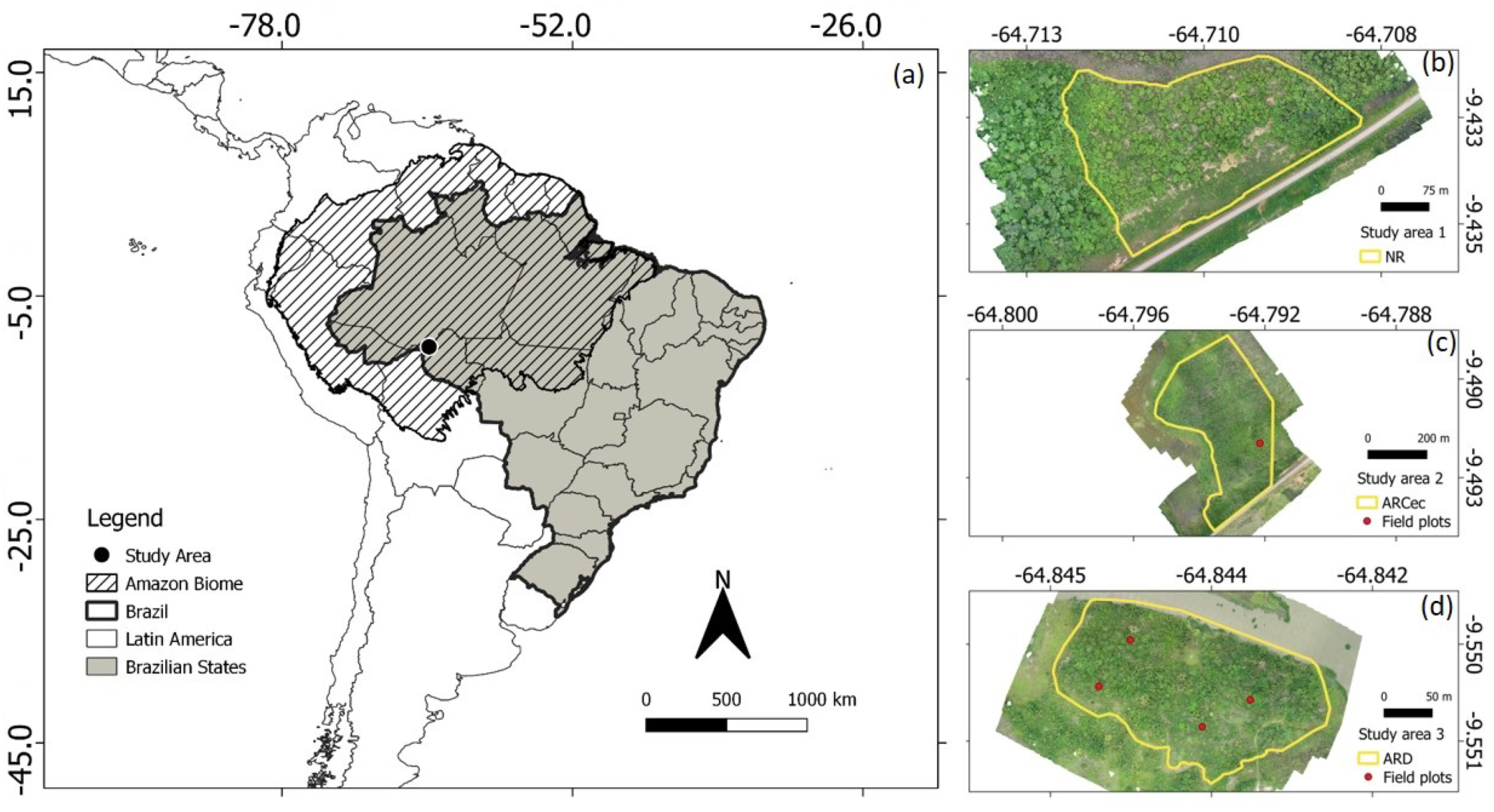
2.1. Study Area

The FR study sites were located in the south Amazon, in the Porto Velho Municipality, along the Madeira river, in Rondônia (RO) state, Brazil (Figure 1).

One site was a naturally regenerating (NR) forest with Vismia sp. occurrence. Another site was an actively restored forest with Cecropia (ARCec). The third site was an actively restored diverse forest (ARD). For better readability, NR, ARCec, and ARD will be referred to as the Vismia site, Cecropia site, and Diverse site, respectively, in plain text, as these abbreviation meanings will keep being used and described in the figures and tables of this manuscript.

The Cecropia site and Diverse site had traditional FR monitoring fieldwork of forest inventory performed in July 2019. The RPA flights were conducted in December 2019.

2.2. Materials

The RPA used in this study was a Phantom 4 Pro (a rotary wing). It was coupled with an RGB 1“CMOS 20MP sensor. For more information about this RPA model, see [40].

Ground control points (GCPs) were collected by the geodetic global navigation satellite system (GNSS) equipment Spectra Precision SP60. For more information about this GNSS equipment, see [41].

The flight planning was drafted using Map Pilot software [42]. Digital surface models (DSMs), digital terrain models (DTMs), and orthorectified mosaics were obtained using Agisoft Metashape [43] software. The deep learning processes were performed using Python [44], and linear regression and graphs in R [45]. The map layouts were generated using QGIS software [46].

2.3. Methods

Figure 2 illustrates the methods applied in this work, described from Section 2.3.2 to Section 2.3.4. From this part until the end of the manuscript, Vismia sp., Cecropia sp. and all kinds of trees in general (regardless of species) will be referred to as Vismia, Cecropia, and All Trees, respectively, for better readability.

2.3.1. Flight Patterns

All flights were in compliance with Brazil’s RPA laws [47] at 80 m above the ground, generating around 2 cm of ground sampling distance (GSD); the front and side overlaps were equal to, respectively, 90% and 80%. Vismia site, Cecropia site, and the Diverse site had 8, 3, and 6 ground control points, respectively.

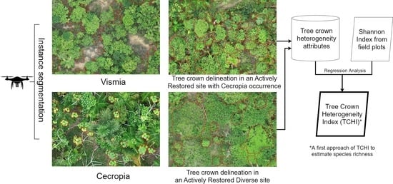
2.3.2. Deep Learning Methods

Deep learning was used to automatically identify three different canopy elements: crown of Vismia, Cecropia, and All Trees. The Mask R-CNN was used on these tasks because it performs instance segmentation and, thus, it counts the number of individuals in an area of interest [37], which is relevant for many ecological studies [28,48,49]. Mask R-CNN was also used because it is a reference instance segmentation algorithm in computer vision research [36,50].

Mask R-CNN is a faster R-CNN extension. Faster R-CNN is an artificial convolutional neural network that identifies each target in an image with a bounding box and classifies it. Mask R-CNN, besides the identification and classification of each target, performs a segmentation process that outputs the shape of the object that is inside each bounding box. The result is an instance segmentation, which allows assessing the shape and the number of targets in an image. For more information about Mask R-CNN, see [38].

Since the Amazon is a high biodiversity biome [31,32,33,34,51,52], it is not possible to know which species are present in a site; thus, the Mask R-CNN for mapping Vismia and Cecropia were assessed as a one-class remote sensing classification process. Such a process is recommended when one specific target is desired among many other complex and unknown features [53,54]. Therefore, in high biodiversity sites, mapping each species using a one-class classification process is a relevant first step. If high accuracy is achieved, future works may develop a single Mask R-CNN that maps Vismia and Cecropia, as well as other relevant species for FR.

For the manual delineation of the samples of Cecropia and Vismia, both had precise GNSS coordinates that were collected to confirm how they look in the RPA images. Figure 3 and Figure 4 illustrates examples of field plot coordinates with manually delineated samples of these targets, as well as ground photos. As Figure 3 and Figure 4 show, Cecropia is much more easily identified visually than Vismia, which suggests that the Cecropia accuracy may be higher.

Regarding All Trees, precise GNSS coordinates were not necessary for manual delineation of samples, which occurred by photointerpretation. The All Trees target was not assessed in the Vismia site because it did not have field plots.

The sampling process is a notable disadvantage of deep learning because a great amount of samples is needed [55]. To help deal with such an issue, Braga et al. [37] developed an algorithm that generates synthetic images with augmentation processes. Such synthetic images improve the neural network classification results because it simulates an increased number of samples. Such a simulation allocates each sample to different locations and performs some brightness changes, vertical or horizontal flips, and rotations in the artificial image. For more details about the use of synthetic images, see Braga et al. [37].

Table 1. Deep learning samples manually delineated according to target and study area.

Delineation Target	Study Area	Epochs	Training Samples	Validation Samples	Test Samples	Samples in Synthetic Images	Total of Synthetic Train Images	Total of Synthetic Validation Images
Vismia sp.	Naturally regenerating site (NR)	150	144	48	48	1	6000	2000
Cecropia sp.	Actively restored site with Cecropia (ARCec)	150	240	80	80	5	1800	600
	Actively restored diverse site (ARD)	-	-	-	50	-	-	-
All Trees	Actively restored site with Cecropia (ARCec)	150	369	123	50	50	9000	3000
	Actively restored diverse site (ARD)	110	150	50	50	50	27,000	9000

illustrates the number of synthetic images generated in this work, as well as the number of samples per synthetic image. Table 1 also illustrates the number of epochs and samples collected for the Mask R-CNN in this work.

The Diverse site only had test samples of Cecropia to evaluate the data shift phenomena, which is a common issue in the remote sensing classification processes: it happens when an algorithm that was trained in a single image is applied to another one and then presents less accurate results due to differences on imaging conditions and local characteristics [56].

Fine-tuning was performed on all Mask R-CNN training processes shown in Table 1 after 30 epochs, which trained only the heads of the convolution neural network with a learning rate equal to 0.001. Then, the whole network was trained. From epochs 31 to 70, the learning rate remained equal to 0.001, but from epochs 71 to 110, the learning rate was divided by 10; from epochs 111 to 150, the learning rate was divided by 100 (except for All Trees at the Diverse site, which had 110 epochs in the training process). ResNet50 and feature pyramid network (FPN) were used as the backbone. The code for the Mask R-CNN process can be seen in Braga et al. [37].

Table 1 and Figure 5 show that each synthetic image had more samples for All Trees than for Cecropia and Vismia. It was due to the spatial resolution of the images, or the GSD. A pixel degradation from 2 to around 30 cm considerably increased the All Trees results accuracy because the 2-centimeter GSD results were inaccurate. Such pixel degradation intended to simulate a satellite image where an accurate All Trees assessment was performed [37]. Moreover, poor results in the original 2-centimeter GSD were somehow expected because individual tree crowns are not clearly distinguishable via photointerpretation after the canopy closes [28,30].

Each synthetic image had more Cecropia than Vismia samples due to the target sizes (Table 1). Cecropia has a smaller crown size than Vismia, so hardware limitations allowed 5 and 1 samples, respectively, on each Cecropia and Vismia 2 cm GSD synthetic image. The amount of Vismia synthetic images, therefore, was considerably higher than Cecropia (see columns “total of synthetic train images” and “total of synthetic validation images” in Table 1). Idem to the amount of synthetic images for All Trees: the Cecropia site area (14.07 ha) is larger than the Diverse site area (3.32 ha); thus, the Cecropia site presented more sample availability (consequently, the Diverse site presented more synthetic images than the Cecropia site for All Trees). Figure 5 shows examples of synthetic images used in this study to train Vismia, Cecropia, and All Trees.

In Cecropia and Vismia mapping, the synthetic images had 1024 × 1024 pixels, as the tests using 128 × 128 pixels images generated inaccurate results. Increasing the background-size for Vismia and Cecropia mapping was necessary to include the different possible background objects that confused the algorithm, such as grass, bare soil, palm trees, and general trees. The processing time of 1024 × 1024 images was slower than 128 × 128 images, but results were much better.

In the All Trees mapping, which was around 30 cm GSD, the synthetic images had 128 × 128 pixels and the background involving only grass generated the most accurate results. After the training and prediction steps, the All Trees polygons with a maximum canopy height model (CHM, which is the difference between DSM and DTM) value less than 2 m and 0.3 m in height in the Cecropia site and the Diverse site, respectively, were excluded because they were bulky grass.

Mapping All Trees in the Diverse site not only involved the Mask R-CNN trained in this site but also the Mask R-CNN trained in the Cecropia site. Since the tree crowns in the Diverse site were usually large, the Mask R-CNN trained in this site usually detected the larger ones, as the smaller ones were omitted in the prediction process. To improve the accuracy of All Trees (by detecting the smaller tree crowns) in the Diverse site, the Mask R-CNN trained in the Cecropia site was also applied. As a result, two different automatic predictions in the same area generated overlapping tree crowns, which was not an “instance segmentation” characteristic. To handle the overlapping results, the tree crowns predicted by the Mask R-CNN trained in the Cecropia site (which detected smaller tree crowns) were excluded when its polygon overlapped with polygons predicted by the Mask R-CNN trained in the Diverse site (which generally detected large tree crowns). This procedure improved the accuracy of the All Trees final result in the Diverse site.

2.3.3. Regression Analysis for Generating the TCHI after Mapping All Trees

Less disturbed and undisturbed forests have species diversity that characterize heterogeneous CHM, while less diverse sites present a homogeneous CHM [16,17]. To evaluate the low-cost RPA capacity for estimating species diversity, a regression analysis between the tree crowns heterogeneity attributes measured by the RPA and the classic Shannon index [57], measured by traditional fieldwork, was performed.

For the regression analysis, the RPA database was generated from the All Trees results (Section 2.3.2), which then had some CHM attributes extracted for each polygon that represented a tree. The attributes of each polygon (of All Trees results) were: area, perimeter, CHM mean, CHM maximum, and principal component analysis (PCA) of the Fourier-based textural ordination (FOTO) statistics (mean and standard deviation). In this work, the defined acronyms of the attributes of the two principal components of FOTO are Fourier textural principal component one (FTPC1) and Fourier textural principal component two (FTPC2).

FOTO evaluated the CHM heterogeneity by a Fourier transform and was implemented using the python package Fototex [58]. FOTO assesses how the pixel values vary along the area and output different values according to the amount of the variation. If the pixels present similar values, FOTO detects a high frequency of these values, which is typical of homogeneous areas, whereas non-frequent values characterize heterogeneous areas. Thus, FOTO numerically expresses patches with more or less heterogeneity. For more information about FOTO, see Bourgoin et al. [16] and Couteron et al. [59].

The traditional fieldwork database consisted of five field plots with a size 25 × 10 m: one plot was located in the Cecropia site (14.07 ha); and four plots were located in the Diverse site (3.32 ha). Cecropia site, although larger, had only one plot because, unfortunately, a fire event between the forest inventory and the RPA flight damaged the vegetation in many patches (it is possible to see patches without trees, some of them with burnt palms, in Appendix A).

A Shannon index [57] (Equation (1)) was calculated for each field plot. The Shannon index considers the species richness and the number of representatives of each species. A site with ten trees that has nine species A, and one species B, is considered less diverse than another site with ten trees that has five species A and five species B. The greater the diversity, the greater the Shannon index value. For more information about the Shannon index, see Spellerberg and Fedor [39] and Pommerening [60].

$$H^{\prime }=-\sum _{i=1}^n{p}_i·ln{p}_i$$

(1)

where $H^{\prime }$ is the Shannon index, $p_i$ is the probability of a randomly selected tree to belong to the tree species i, and n is the number of tree species in the site.

Since the data of five field plots were available, only the automatic trees that intersected these plots were considered on the regression analysis. Thus, each field plot presented a number of trees (automatically identified by the RPA) that corresponded to a Shannon index value (measured by traditional fieldwork). However, the All Trees results are subject to omission errors (when one or more trees are not mapped automatically) and commission errors (when one or more trees do not exist but were automatically mapped); thus, the field plots intersected different amounts of trees. Since the different plots varied on the number of trees associated with a Shannon index value, the average of the crowns’ attributes was used. Thus, for each field plot, the average of each tree crown attribute was used in a simple linear regression to estimate the corresponding Shannon index value. Since the average of each attribute was used, the interpretation of the attribute Fourier textural principal component one mean—FTPC1 mean—and the attribute Fourier textural principal component two mean—FTPC2 mean—may be confusing, but it is relevant to emphasize that each tree crown has a FTPC1 mean value and a FTPC2 mean value. Thus, the average of these values were used in the simple linear regressions to estimate the corresponding Shannon index. Appendix B presents the data that were used in this work.

A simple linear regression shows that results are statistically significant and the variables are significantly related to each other when the p-value is < 0.05 and when a clear linear relation exists between the two variables [61]. For linear regressions with p-value < 0.005, R2adj values close to one and residual standard errors close to zero usually indicate a clear linear relation between two variables [62], while R2 > 0.75 are also usually a good fit in simple linear regressions [63]. If one of the tree crown attributes presents such parameters in the simple linear regression, a preliminary equation that defines the TCHI will show potential for estimating species diversity. However, even if one or more tree crown attributes fill these criteria, it is relevant to emphasize that more field plots are going to be needed in the future to cover a whole range of different FR situations. The TCHI presented in this study is therefore a preliminary result, consisting of a first approach that may lead to relevant studies in the future.

2.3.4. Accuracy Evaluation of the Deep Learning Methods

The omission and commission errors, or the amount of false-positive (FP) and false-negative (FN) occurrences, as well as the overall accuracy [64], allows calculating the recall, precision, and F1 indexes [65], according to Equations (2)–(4), respectively.

$$r=\frac{\mathrm{TP}}{(\mathrm{TP}+\mathrm{FN})}$$

(2)

$$p=\frac{\mathrm{TP}}{(\mathrm{TP}+\mathrm{FP})}$$

(3)

$$\mathrm{F}1=2\ast \frac{(r\ast p)}{(r+p)}$$

(4)

where TP = True Positive, FN = False Negative, FP = False Positive, r = recall, p = precision.

The Mask R-CNN capacity of detecting individual objects must be evaluated as well as the quality of the delineation outlines [37]. In this work, the target objects were the individual crown of Vismia, Cecropia, and All Trees.

A tree crown test sample is properly identified (true-positive) when at least 50% of its area is intersected with an automatically delineated tree crown. Regarding the delineation quality of the true-positives, the accuracy indices recall, precision, F1, and intersection over union (IoU) were used. The IoU calculation is in Figure 6. According to Braga et al. [37], an object is correctly delineated when IoU ≥ 0.5, while IoU > 0.7 indicates high fidelity to the reference data.

Besides evaluating individual object detection and its delineation quality, omission and commission errors must be assessed as areas instead of object detection to avoid overestimation accuracy bias [66]. Object detection considers that the overlap between prediction and test must be higher than 50% while area assessment evaluates the whole reference data, which may degrade the accuracy indices even when overlap is greater than 50%. The area accuracy evaluation also occurred with the indices overall accuracy, recall, precision, and F1.

3. Results

Results of Vismia, Cecropia, and All Trees are illustrated from Figure 7, Figure 8, Figure 9 and Figure 10. The deep learning prediction results for the whole study areas can be seen in Appendix A.

Regarding TCHI after mapping All Trees, Figure 11 shows the simple linear regression results, which should be considered preliminary due to the limited amount of samples. Despite being preliminary, the attribute Fourier textural principal component one mean (FTPC1 mean) presented the most accurate results and showed potential for the low-cost RPA images to estimate species diversity. Figure 11 also shows that the tree crown area and the tree crown perimeter were highly related to the Shannon index.

Results Accuracy

Table 2. Mask R-CNN accuracy for delineation and area distribution. Results were accurate in general, except Vismia’s delineation, which was inaccurate. NR is a naturally regenerating forest with Vismia occurrence, ARCec is an actively restored forest with Cecropia, and ARD is an actively restored diverse forest.

		Cecropia: ARCec	Vismia: NR	Trees: ARCec	Trees: ARD	Cecropia: ARD (Test Only)
Delineation Accuracy	Identified trees	91.25%	72.92%	72.00%	56.00%	80.00%
	Tree crowns correctly delineated	0.918	0.086	0.667	0.607	1.000
	IoU	0.772	0.202	0.563	0.558	0.790
	Precision	0.937	0.221	0.730	0.764	0.989
	Recall	0.820	0.888	0.764	0.738	0.798
	F1	0.875	0.354	0.746	0.751	0.883
Area Accuracy	Overall Accuracy	0.993	0.926	0.902	0.642	0.981
	Precision	0.976	0.760	0.893	0.932	0.943
	Recall	0.752	0.796	0.616	0.565	0.669
	F1	0.849	0.777	0.729	0.704	0.783

shows that Mask R-CNN results were accurate in general, except Vismia delineation, which was poor. However, Vismia area distribution was accurate, which means that its contour errors were somehow compensated, for instance, by projecting a shape part on the left where it should be on the right. Cecropia was very accurate, not only in the Cecropia site, but also in the Diverse site, which only had test samples; thus, the data shift issue did not significantly decrease the prediction accuracy of this target (for Cecropia mapping, the Diverse site was the target image considering the domain adaption terminology). Figure 12 and Figure 13 show in histograms the information in Table 2.

Regarding TCHI after mapping All Trees, the regression analysis showed that, despite the small number of samples, FTPC1mean has high potential in estimating species diversity via low-cost RPA. Thus, the preliminary TCHI is defined in Equation (5).

$$\mathrm{TCHI}=0.7095141\ast \mathrm{FTPC}1\mathrm{mean}+1.5064680$$

(5)

where TCHI is the tree crown heterogeneity index and FTPC1mean is Fourier textural principal component one mean.

4. Discussion

Results showed that, via low-cost RPA images, Mask R-CNN identifies three different canopy elements in the Amazon FR: Vismia crown, Cecropia crown, and the crowns of all trees in general (regardless of species). Moreover, since the automatic delineation of All Trees was accurate, TCHI was assessed and, despite the small number of samples, its preliminary results showed high potential in estimating the Shannon index, which measures the species diversity.

The Mask R-CNN automatic predictions for the whole extension of the three FR sites is available in Appendix A. Cecropia was very accurate because: (1) it has a considerable distinguishing crown that presented specific responses even to SAR data [67]; and (2) many samples were available in the Cecropia site. Vismia automatic delineation was not accurate, but its canopy area was accurately mapped. Vismia mapping was challenging because: (1) Vismia’s crown edges were not easily identifiable via photointerpretation due to an irregular overlap between two or more individuals; and (2) the Vismia site did not contain many Vismia individuals (as did the Cecropia site for Cecropia individuals); thus, fewer samples were available. Regarding the All Trees mapping in the Cecropia site and in the Diverse site, results were accurate.

Mapping the number of representatives of each species is relevant for planning forest management with conservation or economic purposes because it is possible to know the protection status of each representative, as well as patches that have more or less abundance of the species representatives [48,49]. Besides the relevance of mapping the number of representatives of each species (which is possible via instance segmentation), the spatial distribution and the distance between the representatives of each tree species (which is possible via instance segmentation or semantic segmentation) are also relevant for checking fragmentation, adjacency [49], proper distribution of each species, pollination, and FR indicators assessment [48]. The percentage of canopy that Vismia or Cecropia covers is also a relevant indicator of the Amazon FR and is possible via instance segmentation or semantic segmentation.

Like Ferreira et al. [28] and Moura et al. [29], this study demonstrates that RPA has high potential to map relevant species in the Amazon biome automatically. Besides mapping species, this study also showed that low-cost RPA is capable of automatic mapping and delineating individual crowns of all kinds of trees in a tropical high diverse forest. Due to such capacity (of mapping all kinds of trees), a high potential to estimate species diversity in general via TCHI was also demonstrated in this study, although more studies in the future are mandatory to involve a broader range of FR situations that may improve the generalization capacity of the proposed index.

In other studies on Cecropia, Wagner et al. [68] accurately identified Cecropia hololeuca using deep learning (U-Net algorithm, which performs semantic segmentation) applied on a satellite image of the Brazilian Atlantic Forest biome. Moura et al. [29] accurately mapped Cecropia using faster_R-CNN_inception_v2_pets model on an RPA image, which generates a bounding box in its results. In this work, each Cecropia crown was delineated in an instance segmentation process.

Since Cecropia results were very accurate in this study, the Diverse site, where there were not many Cecropia representatives, had only Cecropia test samples to assess the data shift issue. The data shift did not affect the quality of the delineation of Cecropia crowns, but identified a shorter amount of Cecropia individuals and decreased the accuracy of its area distribution. Future studies must assess domain adaptation alternatives to enable the automatic identification of Cecropia without the requirements of sample acquisition.

The All Trees training in the Diverse site was capable of detecting larger trees only, as described in Section 2.3.2. After applying the Mask R-CNN trained in the Cecropia site, the detection of smaller trees improved the accuracy of the All Trees results in the Diverse site. The All Trees accuracy in both the Cecropia site and the Diverse site presented mean IoU equal to 0.56, which is similar to the 0.61 achieved by Braga et al. [37]. Even so, improving tree crown detection and delineation may improve FR monitoring because the proposed TCHI depends on the automatic delineation of tree crowns regardless of species, which reinforces such automatic delineation as a specific research branch.

Despite the limited amount of samples available, the statistical parameters of the preliminary TCHI suggest that the methodology applied in this work, which is unprecedented as far as the authors know, has high potential in estimating species diversity. The preliminary TCHI therefore reinforced the relation between canopy heterogeneity and species diversity, and a hypothesis mentioned by Camarretta et al. [17] that a proper delineation of tree crowns would improve heterogeneity detection, which is related to species diversity. Although presenting accurate statistical parameters, the potential of TCHI in estimating species diversity must be confirmed by future studies because a significant range of different FR situations must be evaluated. Such potential of species diversity estimation would also map, in a single area, where the FR is more-or-less diverse, which would contribute for the concept of precision forest restoration [69].

Nuijten et al. [70] also stated that canopy heterogeneity is related to species composition in FR by using different remote sensing structural metrics and a statistical analysis to classify a hexagonal tessellation in an RPA image of a Canadian boreal forest. While Nuijten et al. [70] defined structural classes inside random hexagons considering statistical CHM attributes in a boreal forest, this work automatically delineated tree crowns and related them to field data of a tropical forest to estimate species diversity.

This study performed instance segmentation processes, where Mask R-CNN was used. Although the Mask R-CNN training process is slow [28,37], this disadvantage will not be an issue if no more samples are needed. In deep learning, sampling and training processes are a notable disadvantage [55], but, ideally, a convolutional neural network should work like in the human face verification in photos [71], where no additional samples are required for accurate prediction results. However, in remote sensing, new samples are frequently required when classifying new images due to different geographic and temporal conditions, which is a phenomenon known as a data shift [56]. To handle the data shift, domain adaptation became a specific field of research [56], for instance, by collecting samples in many places and times of the year [72] or by developing transfer learning python packages to reduce the number of samples required for training [73]. Thus, when considering that an ideal convolutional neural network does not require more samples for training, Mask R-CNN becomes a good deep learning alternative because its prediction process is fast.

Despite being relevant, domain adaptation is a specific field of research. In remote sensing, machine learning processes are a relevant first step to check if the classifier maps the targets accurately. Then, after mapping the targets accurately, a domain adaptation effort may deal with the data shift issue [74]. In this study, this first step was performed as the Mask R-CNN showed high potential to identify individual crowns of important tree genders (Vismia and Cecropia) and of all trees (regardless of species) on Amazonian FR. The automatic mapping of these targets therefore must present domain adaptation studies in the future.

This work generated four different Mask R-CNN with different weights to perform one-class remote sensing classification. Each Mask R-CNN had one target class and one background class for detecting: Vismia (1); Cecropia (2); All Trees in the Cecropia site (3); and All Trees in the Diverse site (4). Instead of developing different Mask R-CNN for different goals, future studies should also evaluate creating one robust Mask R-CNN with more than one target class and more than one background class. In addition, the background class was essential for accurate results, so future studies should collect more samples in other FR areas with different background contexts, which generally are grass and bare soil. Thus, more target and background classes may develop a single robust neural network that quickly identifies relevant Amazon FR monitoring parameters.

5. Conclusions

Mask R-CNN is capable of detecting the crowns of Vismia and Cecropia, as well as the crowns of all kinds of trees, regardless of species in low-cost RPA images. When assessing species diversity estimation after mapping all kinds of trees, the preliminary TCHI showed high potential in mapping more or less diverse sites. These findings play an important role in FR monitoring, as low-cost RPA proved its potential in estimating quality indicators of Amazon FR projects, which improves FR management and monitoring.

Since low-cost RPA has high potential in detecting relevant Amazon biodiversity FR issues, future studies should evaluate more areas and domain adaptation techniques so that deep learning methods may be accurately applied with high generalization capacity. Moreover, after collecting more data by mapping All Trees in different FR situations, the TCHI equation parameters may improve its range of action. When such high generalization capacity is achieved, and no more samples are required, a user-friendly plugin for open-source geographic information system (GIS) software may be created in the future for the automatic detection of Vismia, Cecropia, general trees, and TCHI.

References

1. SER. Princípios da Society for Ecological Restoration (SER) International Sobre a Restauração Ecológica. Technical Report, Embrapa Florestas. 2021. Available online: https://cdn.ymaws.com/www.ser.org/resource/resmgr/custompages/publications/SER_Primer/ser-primer-portuguese.pdf (accessed on 11 October 2021).
2. Muradian, R.; Corbera, E.; Pascual, U.; Kosoy, N.; May, P.H. Reconciling theory and practice: An alternative conceptual framework for understanding payments for environmental services. Ecol. Econ. 2010, 69, 1202–1208. [Google Scholar] [CrossRef]
3. Adams, C.; Rodrigues, S.T.; Calmon, M.; Kumar, C. Impacts of large-scale forest restoration on socioeconomic status and local livelihoods: What we know and do not know. Biotropica 2016, 48, 731–744. [Google Scholar] [CrossRef]
4. Brancalion, P.H.S.; Viani, R.A.G.; Rodrigues, R.R.; Gandolfi, S. Avaliação e monitoramento de áreas em processo de restauração. In Restauração Ecológica de Ecossistemas Degradados; Martins, S., Ed.; Editora UFV: Viçosa, Brazil, 2012; pp. 262–293. Available online: http://www.esalqlastrop.com.br/img/aulas/Cumbuca%206(2).pdf (accessed on 31 October 2021).
5. PRMA. Protocolo de Monitoramento para Programas e Projetos de Restauração Florestal. Monitoring Protocol for Forest Restoration Programs & Projects. Technical Report, PACTO PELA RESTAURAÇÃO DA MATA ATLÂNTICA. 2013. Available online: http://media.wix.com/ugd/5da841_c228aedb71ae4221bc95b909e0635257.pdf (accessed on 10 July 2021).
6. Chaves, R.B.; Durigan, G.; Brancalion, P.H.; Aronson, J. On the need of legal frameworks for assessing restoration projects success: New perspectives from São Paulo state (Brazil). Restor. Ecol. 2015, 23, 754–759. [Google Scholar] [CrossRef]
7. McDonald, T.; Gann, G.; Jonson, J.; Dixon, K. International Standards for the Practice of Ecological Restoration—Including Principles and Ley Concepts; Technical Report; Society for Ecological Restoration: Washington, DC, USA, 2016; Available online: http://www.seraustralasia.com/wheel/image/SER_International_Standards.pdf (accessed on 9 August 2021).
8. Lovejoy, T.E.; Nobre, C. Amazon Tipping Point. Sci. Adv. 2018, 4, eaat2340. [Google Scholar] [CrossRef] [Green Version]
9. Silva-Junior, C.H.L.; Pessôa, A.C.M.; Carvalho, N.S.; Reis, J.B.C.; Anderson, L.O.; Aragão, L.E.O.C. The Brazilian Amazon deforestation rate in 2020 is the greatest of the decade. Nat. Ecol. Evol. 2021, 5, 144–145. [Google Scholar] [CrossRef]
10. Rödig, E.; Cuntz, M.; Rammig, A.; Fischer, R.; Taubert, F.; Huth, A. The importance of forest structure for carbon fluxes of the Amazon rainforest. Environ. Res. Lett. 2018, 13, 054013. [Google Scholar] [CrossRef]
11. Jakovac, C.C.; Bongers, F.; Kuyper, T.W.; Mesquita, R.C.; Peña-Claros, M. Land use as a filter for species composition in Amazonian secondary forests. J. Veg. Sci. 2016, 27, 1104–1116. [Google Scholar] [CrossRef] [Green Version]
12. Poorter, L.; Bongers, F.; Aide, T.M.; Zambrano, A.M.A.; Balvanera, P.; Becknell, J.M.; Boukili, V.; Brancalion, P.H.; Broadbent, E.N.; Chazdon, R.L.; et al. Biomass resilience of Neotropical secondary forests. Nature 2016, 530, 211–214. [Google Scholar] [CrossRef]
13. Freitas, M.G.; Rodrigues, S.B.; Campos-Filho, E.M.; do Carmo, G.H.P.; da Veiga, J.M.; Junqueira, R.G.P.; Vieira, D.L.M. Evaluating the success of direct seeding for tropical forest restoration over ten years. For. Ecol. Manag. 2019, 438, 224–232. [Google Scholar] [CrossRef]
14. Vieira, D.L.M.; Rodrigues, S.B.; Jakovac, C.C.; da Rocha, G.P.E.; Reis, F.; Borges, A. Active Restoration Initiates High Quality Forest Succession in a Deforested Landscape in Amazonia. Forests 2021, 12, 1022. [Google Scholar] [CrossRef]
15. Mesquita, R.C.; Ickes, K.; Ganade, G.; Williamson, G.B. Alternative successional pathways in the Amazon Basin. J. Ecol. 2001, 89, 528–537. [Google Scholar] [CrossRef] [Green Version]
16. Bourgoin, C.; Betbeder, J.; Couteron, P.; Blanc, L.; Dessard, H.; Oszwald, J.; Le Roux, R.; Cornu, G.; Reymondin, L.; Mazzei, L.; et al. UAV-based canopy textures assess changes in forest structure from long-term degradation. Ecol. Indic. 2020, 115, 106386. [Google Scholar] [CrossRef] [Green Version]
17. Camarretta, N.; Harrison, P.A.; Bailey, T.; Potts, B.; Lucieer, A.; Davidson, N.; Hunt, M. Monitoring forest structure to guide adaptive management of forest restoration: A review of remote sensing approaches. New For. 2020, 51, 573–596. [Google Scholar] [CrossRef]
18. Zahawi, R.A.; Dandois, J.P.; Holl, K.D.; Nadwodny, D.; Reid, J.L.; Ellis, E.C. Using lightweight unmanned aerial vehicles to monitor tropical forest recovery. Biol. Conserv. 2015, 186, 287–295. [Google Scholar] [CrossRef] [Green Version]
19. Chen, S.; McDermid, G.; Castilla, G.; Linke, J. Measuring vegetation height in linear disturbances in the boreal forest with UAV photogrammetry. Remote Sens. 2017, 9, 1257. [Google Scholar] [CrossRef] [Green Version]
20. Wu, X.; Shen, X.; Cao, L.; Wang, G.; Cao, F. Assessment of individual tree detection and canopy cover estimation using unmanned aerial vehicle based light detection and ranging (UAV-LiDAR) data in planted forests. Remote Sens. 2019, 11, 908. [Google Scholar] [CrossRef] [Green Version]
21. Belmonte, A.; Sankey, T.; Biederman, J.A.; Bradford, J.; Goetz, S.J.; Kolb, T.; Woolley, T. UAV-derived estimates of forest structure to inform ponderosa pine forest restoration. Remote Sens. Ecol. Conserv. 2020, 6, 181–197. [Google Scholar] [CrossRef]
22. Albuquerque, R.W.; Ferreira, M.E.; Olsen, S.I.; Tymus, J.R.C.; Balieiro, C.P.; Mansur, H.; Moura, C.J.R.; Costa, J.V.S.; Branco, M.R.C.; Grohmann, C.H. Forest Restoration Monitoring Protocol with a Low-Cost Remotely Piloted Aircraft: Lessons Learned from a Case Study in the Brazilian Atlantic Forest. Remote Sens. 2021, 13, 2401. [Google Scholar] [CrossRef]
23. Almeida, D.R.A.D.; Stark, S.C.; Chazdon, R.; Nelson, B.W.; César, R.G.; Meli, P.; Gorgens, E.; Duarte, M.M.; Valbuena, R.; Moreno, V.S.; et al. The effectiveness of lidar remote sensing for monitoring forest cover attributes and landscape restoration. For. Ecol. Manag. 2019, 438, 34–43. [Google Scholar] [CrossRef]
24. LeCun, Y.; Bengio, Y.; Hinton, G. Deep learning. Nature 2015, 521, 436–444. [Google Scholar] [CrossRef]
25. Zhao, B.; Feng, J.; Wu, X.; Yan, S. A survey on deep learning-based fine-grained object classification and semantic segmentation. Int. J. Autom. Comput. 2017, 14, 119–135. [Google Scholar] [CrossRef]
26. Zhu, X.X.; Tuia, D.; Mou, L.; Xia, G.S.; Zhang, L.; Xu, F.; Fraundorfer, F. Deep learning in remote sensing: A comprehensive review and list of resources. IEEE Geosci. Remote Sens. Mag. 2017, 5, 8–36. [Google Scholar] [CrossRef] [Green Version]
27. Brodrick, P.G.; Davies, A.B.; Asner, G.P. Uncovering ecological patterns with convolutional neural networks. Trends Ecol. Evol. 2019, 34, 734–745. [Google Scholar] [CrossRef]
28. Ferreira, M.P.; de Almeida, D.R.A.; de Almeida Papa, D.; Minervino, J.B.S.; Veras, H.F.P.; Formighieri, A.; Santos, C.A.N.; Ferreira, M.A.D.; Figueiredo, E.O.; Ferreira, E.J.L. Individual tree detection and species classification of Amazonian palms using UAV images and deep learning. For. Ecol. Manag. 2020, 475, 118397. [Google Scholar] [CrossRef]
29. Moura, M.M.; de Oliveira, L.E.S.; Sanquetta, C.R.; Bastos, A.; Mohan, M.; Corte, A.P.D. Towards Amazon Forest Restoration: Automatic Detection of Species from UAV Imagery. Remote Sens. 2021, 13, 2627. [Google Scholar] [CrossRef]
30. Schiefer, F.; Kattenborn, T.; Frick, A.; Frey, J.; Schall, P.; Koch, B.; Schmidtlein, S. Mapping forest tree species in high resolution UAV-based RGB-imagery by means of convolutional neural networks. ISPRS J. Photogramm. Remote Sens. 2020, 170, 205–215. [Google Scholar] [CrossRef]
31. Haffer, J. Speciation in Amazonian forest birds. Science 1969, 165, 131–137. [Google Scholar] [CrossRef]
32. Prance, G.T. A comparison of the efficacy of higher taxa and species numbers in the assessment of biodiversity in the neotropics. Philos. Trans. R. Soc. Lond. Ser. B Biol. Sci. 1994, 345, 89–99. [Google Scholar]
33. Antonelli, A.; Zizka, A.; Carvalho, F.A.; Scharn, R.; Bacon, C.D.; Silvestro, D.; Condamine, F.L. Amazonia is the primary source of Neotropical biodiversity. Proc. Natl. Acad. Sci. USA 2018, 115, 6034–6039. [Google Scholar] [CrossRef] [Green Version]
34. Ter Steege, H.; de Oliveira, S.M.; Pitman, N.C.; Sabatier, D.; Antonelli, A.; Andino, J.E.G.; Aymard, G.A.; Salomão, R.P. Towards a dynamic list of Amazonian tree species. Sci. Rep. 2019, 9, 3501. [Google Scholar] [CrossRef] [Green Version]
35. Ruiz-Santaquiteria, J.; Bueno, G.; Deniz, O.; Vallez, N.; Cristobal, G. Semantic versus instance segmentation in microscopic algae detection. Eng. Appl. Artif. Intell. 2020, 87, 103271. [Google Scholar] [CrossRef]
36. Hafiz, A.M.; Bhat, G.M. A survey on instance segmentation: State of the art. Int. J. Multimed. Inf. Retr. 2020, 9, 171–189. [Google Scholar] [CrossRef]
37. Braga, J.R.G.; Peripato, V.; Dalagnol, R.; Ferreira, M.P.; Tarabalka, Y.; Aragão, L.E.O.C.; Campos Velho, H.F.; Shiguemori, E.H.; Wagner, F.H. Tree Crown Delineation Algorithm Based on a Convolutional Neural Network. Remote Sens. 2020, 12, 1288. [Google Scholar] [CrossRef] [Green Version]
38. He, K.; Gkioxari, G.; Dollár, P.; Girshick, R. Mask r-cnn. In Proceedings of the IEEE International Conference on Computer Vision, Venice, Italy, 22–29 October 2017; pp. 2961–2969. [Google Scholar]
39. Spellerberg, I.F.; Fedor, P.J. A tribute to Claude Shannon (1916–2001) and a plea for more rigorous use of species richness, species diversity and the ‘Shannon–Wiener’Index. Glob. Ecol. Biogeogr. 2003, 12, 177–179. [Google Scholar] [CrossRef] [Green Version]
40. DJI. Phantom 4PRO. Available online: https://www.dji.com/br/phantom-4-pro (accessed on 12 January 2022).
41. SPECTRA GEOSPATIAL. SP60 Product Details. Available online: https://spectrageospatial.com/sp60-gnss-receiver/ (accessed on 12 January 2022).
42. DRONESMADEEASY. Map Pilot for DJI. 2020. Available online: https://support.dronesmadeeasy.com/hc/en-us/categories/200739936-Map-Pilot-for-iOS (accessed on 25 February 2021).
43. AGISOFT. Discover Intelligent Photogrammetry with Metashape. 2020. Available online: https://www.agisoft.com/ (accessed on 25 February 2021).
44. Python Core Team. Python: A dynamic, Open Source Programming Language. Python Softw. Found. Available online: https://www.python.org/ (accessed on 17 June 2021).
45. R Core Team. R: A language and Environment for Statistical Computing; R Foundation for Statistical Computing: Vienna, Austria, 2013; Available online: http://www.R-project.org (accessed on 17 June 2021).
46. QGIS Development Team. QGIS Geographic Information System. QGIS Association. 2021. Available online: https://www.qgis.org (accessed on 17 June 2021).
47. ANAC. Agência Nacional de Aviação Civil. Requisitos Gerais para Aeronaves não Tripuladas de uso Civil. Resolução Número 419, de 2 de maio de 2017. Regulamento Brasileiro da Aviação Civil Especial, RBAC-E Número 94. 2017. Available online: https://www.anac.gov.br/assuntos/legislacao/legislacao-1/rbha-e-rbac/rbac/rbac-e-94/@@display-file/arquivo_norma/RBACE94EMD00.pdf (accessed on 17 June 2021).
48. Guariguata, M.R.; Pinard, M.A. Ecological knowledge of regeneration from seed in neotropical forest trees: Implications for natural forest management. For. Ecol. Manag. 1998, 112, 87–99. [Google Scholar] [CrossRef]
49. Varma, V.K.; Ferguson, I.; Wild, I. Decision support system for the sustainable forest management. For. Ecol. Manag. 2000, 128, 49–55. [Google Scholar] [CrossRef]
50. Minaee, S.; Boykov, Y.Y.; Porikli, F.; Plaza, A.J.; Kehtarnavaz, N.; Terzopoulos, D. Image Segmentation Using Deep Learning: A Survey. IEEE Trans. Pattern Anal. Mach. Intell. 2021. [Google Scholar] [CrossRef]
51. Antonelli, A.; Sanmartín, I. Why are there so many plant species in the Neotropics? Taxon 2011, 60, 403–414. [Google Scholar] [CrossRef]
52. Ter Steege, H.; Sabatier, D.; Mota de Oliveira, S.; Magnusson, W.E.; Molino, J.F.; Gomes, V.F.; Pos, E.T.; Salomão, R.P. Estimating species richness in hyper-diverse large tree communities. Ecology 2017, 98, 1444–1454. [Google Scholar] [CrossRef]
53. Bellinger, C.; Sharma, S.; Japkowicz, N. One-Class versus Binary Classification: Which and When? In Proceedings of the 2012 11th International Conference on Machine Learning and Applications, Boca Raton, FL, USA, 12–15 December 2012; Volume 2, pp. 102–106. [Google Scholar] [CrossRef]
54. Deng, X.; Li, W.; Liu, X.; Guo, Q.; Newsam, S. One-class remote sensing classification: One-class vs. binary classifiers. Int. J. Remote. Sens. 2018, 39, 1890–1910. [Google Scholar] [CrossRef]
55. Dargan, S.; Kumar, M.; Ayyagari, M.R.; Kumar, G. A survey of deep learning and its applications: A new paradigm to machine learning. Arch. Comput. Methods Eng. 2020, 27, 1071–1092. [Google Scholar] [CrossRef]
56. Zhang, J.; Liu, J.; Pan, B.; Shi, Z. Domain Adaptation Based on Correlation Subspace Dynamic Distribution Alignment for Remote Sensing Image Scene Classification. IEEE Trans. Geosci. Remote Sens. 2020, 58, 7920–7930. [Google Scholar] [CrossRef]
57. Shannon, C.E. A mathematical theory of communication. Bell Syst. Tech. J. 1948, 27, 379–423. [Google Scholar] [CrossRef] [Green Version]
58. PyPI. Fototex. Available online: https://pypi.org/project/fototex/ (accessed on 12 January 2022).
59. Couteron, P.; Barbier, N.; Gautier, D. Textural ordination based on Fourier spectral decomposition: A method to analyze and compare landscape patterns. Landsc. Ecol. 2006, 21, 555–567. [Google Scholar] [CrossRef]
60. Pommerening, A. Approaches to quantifying forest structures. For. Int. J. For. Res. 2002, 75, 305–324. [Google Scholar] [CrossRef]
61. Alexopoulos, E.C. Introduction to multivariate regression analysis. Hippokratia 2010, 14, 23. [Google Scholar]
62. Pal, M.; Bharati, P. Introduction to correlation and linear regression analysis. In Applications of Regression Techniques; Springer: Singapore, 2019; pp. 1–18. [Google Scholar]
63. Lewis, S. Regression analysis. Pract. Neurol. 2007, 7, 259–264. [Google Scholar] [CrossRef]
64. Congalton, R.G. A review of assessing the accuracy of classifications of remotely sensed data. Remote Sens. Environ. 1991, 37, 35–46. [Google Scholar] [CrossRef]
65. Goutte, C.; Gaussier, E. A probabilistic interpretation of precision, recall and F-score, with implication for evaluation. In European Conference on Information Retrieval; Springer: Berlin/Heidelberg, Germany, 2005; pp. 345–359. [Google Scholar]
66. Radoux, J.; Bogaert, P. Good practices for object-based accuracy assessment. Remote Sens. 2017, 9, 646. [Google Scholar] [CrossRef] [Green Version]
67. Foody, G.M.; Green, R.M.; Lucas, R.; Curran, P.J.; Honzák, M.; Do Amaral, I. Observations on the relationship between SIR-C radar backscatter and the biomass of regenerating tropical forests. Int. J. Remote Sens. 1997, 18, 687–694. [Google Scholar] [CrossRef]
68. Wagner, F.H.; Sanchez, A.; Tarabalka, Y.; Lotte, R.G.; Ferreira, M.P.; Aidar, M.P.; Gloor, E.; Phillips, O.L.; Aragao, L.E. Using the U-net convolutional network to map forest types and disturbance in the Atlantic rainforest with very high resolution images. Remote Sens. Ecol. Conserv. 2019, 5, 360–375. [Google Scholar] [CrossRef] [Green Version]
69. Castro, J.; Morales-Rueda, F.; Navarro, F.B.; Löf, M.; Vacchiano, G.; Alcaraz-Segura, D. Precision restoration: A necessary approach to foster forest recovery in the 21st century. Restor. Ecol. 2021, 29, e13421. [Google Scholar] [CrossRef]
70. Nuijten, R.J.; Coops, N.C.; Watson, C.; Theberge, D. Monitoring the Structure of Regenerating Vegetation Using Drone-Based Digital Aerial Photogrammetry. Remote Sens. 2021, 13, 1942. [Google Scholar] [CrossRef]
71. Guo, G.; Zhang, N. A survey on deep learning based face recognition. Comput. Vis. Image Underst. 2019, 189, 102805. [Google Scholar] [CrossRef]
72. Brandt, M.; Tucker, C.J.; Kariryaa, A.; Rasmussen, K.; Abel, C.; Small, J.; Chave, J.; Rasmussen, L.V.; Hiernaux, P.; Diouf, A.A.; et al. An unexpectedly large count of trees in the West African Sahara and Sahel. Nature 2020, 587, 78–82. [Google Scholar] [CrossRef]
73. Weinstein, B.G.; Marconi, S.; Aubry-Kientz, M.; Vincent, G.; Senyondo, H.; White, E.P. DeepForest: A Python package for RGB deep learning tree crown delineation. Methods Ecol. Evol. 2020, 11, 1743–1751. [Google Scholar] [CrossRef]
74. Zhu, L.; Ma, L. Class centroid alignment based domain adaptation for classification of remote sensing images. Pattern Recognit. Lett. 2016, 83, 124–132. [Google Scholar] [CrossRef]
Figure 1. Location of the FR study sites: (a) in South America, Brazil, and Amazon biome. (b) Study site 1 (8.19 hectares) is a naturally regenerating (NR) forest with Vismia spp. occurrence, which will be called, in this work, the Vismia site (no field plots of forest inventory were available on this site). (c) Study site 2 (14.07 hectares) is an actively restored site with Cecropia spp. (ARCec) occurrence, which will be called, in this work, the Cecropia site (only one field plot was not damaged after a fire event on this site). (d) Study site 3 (3.32 hectares) is an actively restored diverse (ARD) site, which will be called, in this work, the Diverse site.
Remotesensing 14 00830 g001
Figure 2. Deep learning methods for automatically mapping of Vismia, Cecropia and All Trees and regression analysis methods to assess the tree crown heterogeneity index (TCHI) after mapping All Trees.
Remotesensing 14 00830 g002
Figure 3. Example of Vismia: manually delineated samples with precise GNSS coordinates that confirm how these targets look in the RPA image (a); and ground photo (b).
Remotesensing 14 00830 g003
Figure 4. Example of Cecropia: manually delineated samples with precise GNSS coordinates that confirm how these targets look in the RPA image (a); and ground photo (b).
Remotesensing 14 00830 g004
Figure 5. Examples of synthetic images that were used to train Vismia, Cecropia, and All Trees. In these images, the samples are artificially added to a background image.
Remotesensing 14 00830 g005
Figure 6. Recall, precision, and IoU to evaluate the quality of the automatic delineation.
Remotesensing 14 00830 g006
Figure 7. (a) Vismia training process; (b) and the prediction results in the naturally regenerating (NR) site. The loss values reduced considerably from epoch 31 due to the transfer learning process, where the whole network started to be trained instead of only the heads.
Remotesensing 14 00830 g007
Figure 8. (a) Cecropia training process; (b) and the prediction results in the actively restored site with Cecropia (ARCec). The loss values reduced considerably from epoch 31 due to the transfer learning process, where the whole network started to be trained instead of only the heads.
Remotesensing 14 00830 g008
Figure 9. (a) All Trees training process in the actively restored site with Cecropia (ARCec); (b) and the corresponding prediction results. The loss values reduced considerably from epoch 31 due to the transfer learning process, where the whole network started to be trained instead of only the heads.
Remotesensing 14 00830 g009
Figure 10. (a) All Trees training process in the Actively restored diverse (ARD) site, which was not accurate; and (b) the prediction results that also used the convolutional neural network trained in ARCec (Figure 9) to map small trees, as mentioned in Section 2.3.2 (b). The loss values reduced considerably from epoch 31 due to the transfer learning process, where the whole network started to be trained instead of only the heads.
Remotesensing 14 00830 g010
Figure 11. Simple linear regression results. Each simple linear regression relates the average value of a crown attribute of the trees that were automatically delineated in a field plot to the corresponding Shannon index.
Remotesensing 14 00830 g011
Figure 12. Mask R-CNN accuracy on the delineation of the targets: (a) identified trees; (b) tree crowns correctly delineated; (c) intersection over union; (d) precision; (e) recall; (f) and F1. ARCec is actively restored site with Cecropia and ARD is actively restored diverse site.
Remotesensing 14 00830 g012
Figure 13. Mask R-CNN accuracy on the area distribution of the targets: (a) overall accuracy; (b) precision; (c) recall; (d) and F1. ARCec is actively restored site with Cecropia and ARD is actively restored diverse site.
Remotesensing 14 00830 g013