Article

Interannual Relationship between Haze Days in December–January and Satellite-Based Leaf Area Index in August–September over Central North China

School of Atmospheric Sciences, Sun Yat-sen University, and Southern Marine Science and Engineering Guangdong Laboratory (Zhuhai), Zhuhai 519082, China
*
Author to whom correspondence should be addressed.
Remote Sens. 2022, 14(4), 884; https://doi.org/10.3390/rs14040884
Submission received: 17 December 2021 / Revised: 4 February 2022 / Accepted: 8 February 2022 / Published: 12 February 2022

Abstract

:
Haze pollution in central North China has become a hot topic in recent decades due to its serious environmental and health effects. In this work, the interannual relationship between haze days in December–January (DJ_HD) and leaf area index in August–September (AS_LAI) over central North China, along with the possible physical mechanisms involved, are investigated. The relationship varies in different periods, being significant during 1982–2000 (P1) but insignificant during 2001–2014 (P2). During P1, there is an in-phase relationship between AS_LAI and surface evaporation, and an out-of-phase relationship between AS_LAI and surface albedo in August–September. The surface evaporation and albedo anomalies persist to October–November and are associated with lower top-layer volumetric soil water, upward sensible heat flux and downward latent heat flux anomalies in October–November, which act as the bridge in the relationship between AS_LAI and DJ_HD. Both the volumetric soil water and heat fluxes anomalies persist to December–January and correspond to atmospheric circulations similar to the weakened East Asian winter monsoon pattern, which is the dominant system for winter haze events. Thus, the ventilation conditions in December–January are favorable for the accumulation of haze particles. However, during P2, the relationships are not significant between AS_LAI and volumetric soil water or surface soil temperature during October–January. Meanwhile, the East Asian winter monsoon is likely strengthened and tends to be more significantly affected by factors including Arctic sea ice, Arctic Oscillation, etc. Therefore, the effects of AS_LAI on the monsoon may become insignificant and, in turn, the relationship between AS_LAI and DJ_HD becomes insignificant during P2.

1. Introduction

Haze is a phenomenon whereby a large number of fine particles float evenly in the air and reduce visibility [1]. Haze pollution has become a hot topic in China, having caused serious environmental and health problems [2,3,4]. The increasing concentration of haze particles leads to changes in the amount of solar irradiance reaching the Earth’s surface; the temperature structure of the atmosphere; rainfall; and the hydrological cycle, which connects directly to the availability and quality of fresh water—a major global environmental issue [5,6,7]. Meanwhile, haze particles have been found to be capable of penetrating the lungs and bloodstream and, in turn, cause respiratory and cardiovascular diseases [8,9,10]. The human population is dense in central North China, and the frequent haze pollution in winter here exerts a considerable influence on people’s daily lives [11,12,13,14]. For example, in the winter of 2013, a series of extreme haze events happened in eastern China and Beijing witnessed its first orange haze warning (the second-highest level) in its meteorological history [15,16,17]. These severe haze events with thick clouds of smog spread over millions of square kilometers and affected the health of millions, leading to a significant increase in the number of patients with respiratory and cardiovascular diseases [18,19,20].
To alleviate the influence and improve the prediction skill for haze events, the mechanisms of haze pollution have been investigated in recent studies [21,22,23]. On long-term timescales, haze events are dominated by anthropogenic emissions including agricultural burning, chemical production, coal combustion, and so on [24,25,26]. On the other hand, the interannual–decadal variabilities of haze pollution are mainly affected by climatic aspects [27,28,29]. Local and large-scale atmospheric circulations dominate the dispersion of haze particles [30,31,32]. Meanwhile, some of the precursory climate drivers of haze pollution have been revealed in recent studies [23]. For example, Yang and Yuan [33] revealed that the number of haze days in the North China Plain region in late winter is closely related to Arctic sea ice in October, and the Pacific Sea surface temperature plays a key role in delivering the effects of the sea ice on the atmospheric circulation and diffusion conditions linked with the accumulation and growth of haze pollutants. Zhao et al. [34] indicated that during the negative phase of the Pacific Decadal Oscillation, the weakened Mongolia High and corresponding ascending motion anomalies tend to make the air unstable and conducive to the spread of haze pollutants in eastern China. Furthermore, land–atmosphere interactions have also been suggested to substantially modulate haze pollution in China. Zhang et al. [35] revealed that autumn negative soil moisture anomalies could induce the positive phase of the eastern Atlantic/western Russia pattern, meaning the associated anticyclonic circulations would occur more frequently and strongly to limit the conditions needed locally for the vertical and horizontal dispersion of haze. Yin and Wang [36] indicated that the relationship between Eurasian snow cover and the number of haze days in winter in central North China strengthened significantly after the mid-1990s. They attributed this to effective connections among the snow cover, soil moisture and land-surface radiation related to the northward shift of the East Asian jet stream, which induces anticyclonic circulation anomalies over central North China.
Vegetation plays a vital role in the exchanges of energy and matter between land and atmosphere owing to its albedo and radiation effects, transpiration, roughness length, and so on [37,38,39]. These biophysical processes modulate local and global air temperatures, processes in the atmospheric boundary layer, cloud cover, rainfall, differential heating, and atmospheric circulations to different degrees [40,41,42]. In central North China, the vegetation mainly consists of evergreen–deciduous mixed forest, temperate deciduous forest, and croplands. The spatiotemporal variations of the vegetation in central North China have been found to be related to the local air temperature, rainfall, and strength of drought events [43,44,45]. It is known that from a biochemical perspective, vegetation provides a source for haze pollution through the formation of secondary organic aerosols—that is, biogenic volatile organic compounds [46,47]. However, from the biophysical perspective, the relationships between vegetation and haze pollution in central North China and the possible feedback processes are complex and largely unexplored. There have been a few studies on the effects of vegetation on winter climate, when the frequency of haze events in central North China is at its highest [48]. For example, Bonan et al. [49] carried out global climate model simulations and found that the removal of vegetation reduces the global winter temperature through change in the surface albedo. Considering the vegetation feeds back to the local and large-scale climate, we speculate that it is highly possible that vegetation is linked to winter haze pollution in central North China.
Therefore, this study aims to reveal the possible relationship between vegetation and the number of winter haze days in central North China, as well as the possible underlying physical processes involved, to improve our level of understanding of the mechanisms of land–atmosphere interactions and the prediction skill for haze events in central North China. The rest of the paper is organized as follows: In Section 2, the data and methods used in this study are introduced. In Section 3, the spatiotemporal variabilities of haze pollution in central North China are illustrated, followed by an examination of the relationship between haze pollution and vegetation and the possible physical processes involved. Finally, conclusions and some further discussions are provided in Section 4.

2. Materials and Methods

In this work, haze days are defined as days with visibility less than 10 km, relative humidity less than 90%, surface wind speed less than 7 m s−1, and an absence of precipitation [50,51,52]. The humidity threshold of 90% is for distinguishing haze from fog, and the surface wind speed threshold of 7 m s−1 is for distinguishing haze from dust [53,54]. The observed visibility, relative humidity (calculated based on temperature and dewpoint temperature), surface wind speed, and precipitation data are derived from the National Climatic Data Center (NCDC) Global Summary of Day (GSOD) database during 1980 to 2018. After quality control, there are 119 meteorological stations available over the mainland of eastern China and 42 meteorological stations available over central North China (31°–42°N, 112°–121°E). Monthly haze days are calculated as the sum of the haze days in that month, and the regional mean index—the December–January haze days index (hereafter referred to as DJ_HD)—is computed as the average haze days of the meteorological stations within the region.
Leaf area index (LAI) products have been widely used to characterize biophysical variations of vegetation. In this work, the Global Land Surface Satellite (GLASS) LAI product spanning from 1982 to 2014 is used to assess vegetation growth [55]. This long-term product is generated based on Advanced Very High Resolution Radiometer reflectance data in a geographic latitude/longitude projection during 1982–1999, and Moderate Resolution Imaging Spectroradiometer surface-reflectance data in a sinusoidal projection during 2000–2014. The original GLASS LAI data at a spatial resolution of 0.05° and a temporal resolution of eight days are processed to a spatial resolution of 1° and a temporal resolution of one month for the convenience of analysis. Meanwhile, the LAI3g product [56] is used to verify if the relationship between haze days and LAI is independent of dataset selection. The LAI3g dataset is generated biweekly at a 1/12° spatial resolution from the third-generation normalized difference vegetation index dataset supplied by the Global Inventory Modeling and Mapping Studies, which is also processed into a spatial resolution of 1° and a temporal resolution of one month. The regional mean index—the August–September LAI index (hereafter referred to as AS_LAI)—is calculated as the average LAI of the grids within central North China using the weighting approach of the area of each grid cell.
Meteorological data in this work are mainly derived from the ERA5 reanalysis data, including variables of monthly 2-m temperature, sea level pressure, zonal and meridional wind, geopotential height, 10-m wind speed, evaporation, sensible and latent heat flux, surface longwave and shortwave radiation, the volume of water in the soil layer 1 (0–7 cm), and the temperature of the soil at level 1 (0–7 cm) at the spatial resolution of 1° [57]. Monthly surface albedo data are derived from the Satellite Application Facility on Climate Monitoring datasets of the European Meteorological Satellite at the spatial resolution of 0.25°, which is also processed into a spatial resolution of 1° [58]. The time span of all data used in this work is 1982–2014, which is consistent with the time span of the GLASS LAI product.
In this study, the multivariate empirical orthogonal function (MV-EOF) is used to capture the coupled modes and corresponding time coefficients between December and January haze days [59]. Linear regression, Pearson correlation, composite analyses, and 13-year-sliding correlation are applied to explore the linkage between haze days and LAI, as well as the related climate fields. Statistical significance is determined by the Student’s t-test. In correlation analyses, the Pearson correlation coefficients and significance levels are shown as the key statistics in climatic dynamic analyses considering that it is hardly possible to present all the correlation matrices at all the grid points. Further, in the regression analyses, the linear regression coefficients and significance levels are shown as the key statistics. All the analyses are carried out using detrended data. Meanwhile, the net energy flux (Qnet) at the surface is calculated based on the following equation:
Qnet  =  DLR  −  ULR  +  DSR  −  USR  + SH + LH,
where Qnet represents the net heat flux transferred from the atmosphere to the surface, DLR represents the downward longwave radiation, ULR represents the upward longwave radiation, DSR represents the downward shortwave radiation, USR represents the upward shortwave radiation, SH represents the downward sensible heat flux, and LH represents the downward latent heat flux.

3. Results

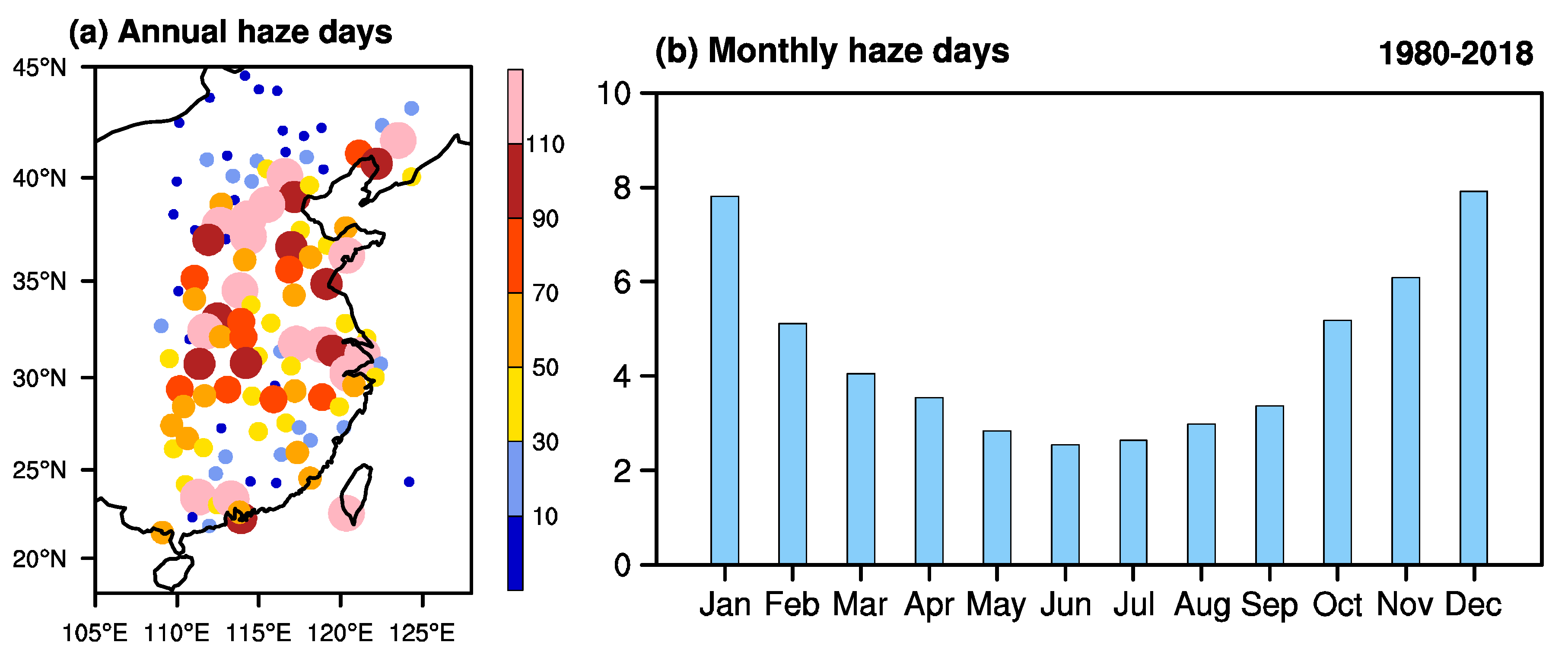
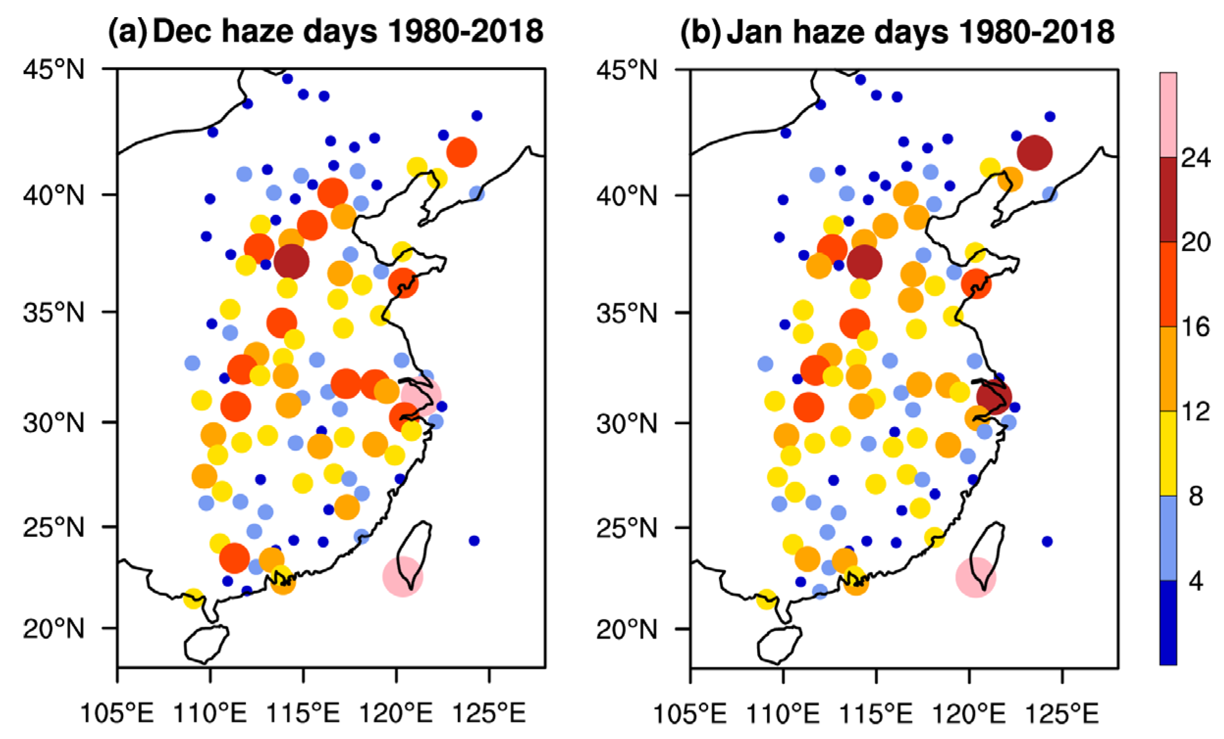
3.1. Spatiotemporal Characteristics of Haze Days in Eastern China

Studies have suggested that more than 40% of haze day occurrences can be observed in boreal winter in China owing to the favorable meteorological conditions [27]. In eastern China, the average number of haze days at 119 stations is the most in autumn and winter, with the maximum happening in December–January when it reaches 7.9 days, and the minimum in June (Figure 1). Hence, we focus on December–January haze days.
Meanwhile, among all stations, the stations in central North China (31°–42°N, 112°–121°E) experience the most haze days in December–January, with an average of 9.2 days and a maximum of 23.2 days (Figure 1 and Figure 2). The spatial patterns of the first mode of the MV-EOF of December and January haze days in central North China show positive values presented over most stations and in-phase spatial patterns from December to January (Figure 3). The leading mode accounts for 29.7% of the total covariance for the December and January haze days together. The time series of the first EOF exhibits the characteristic of interannual variability. Given the importance of central North China to the country in terms of its influence on national economic development, as well as the considerable losses that can be incurred in relation to haze days, this work focuses on the DJ_HD in central North China.

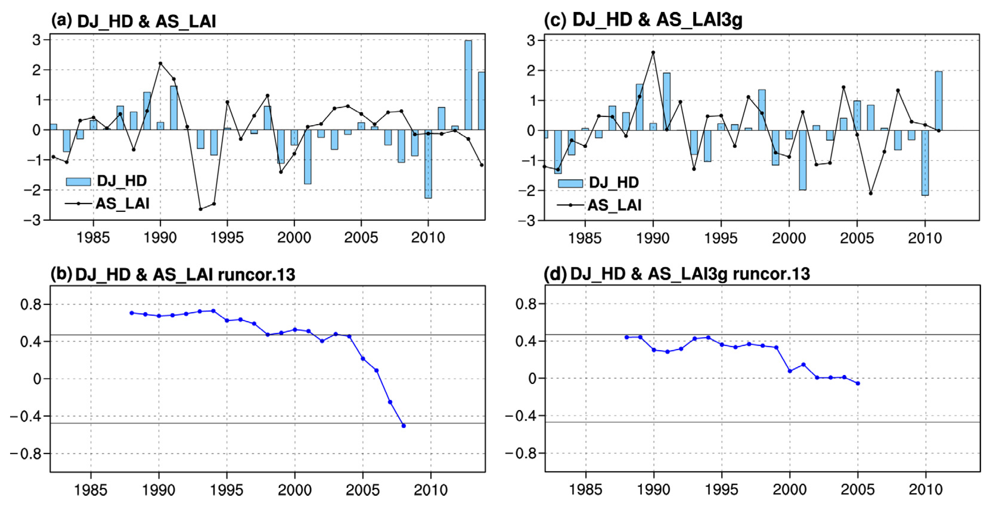
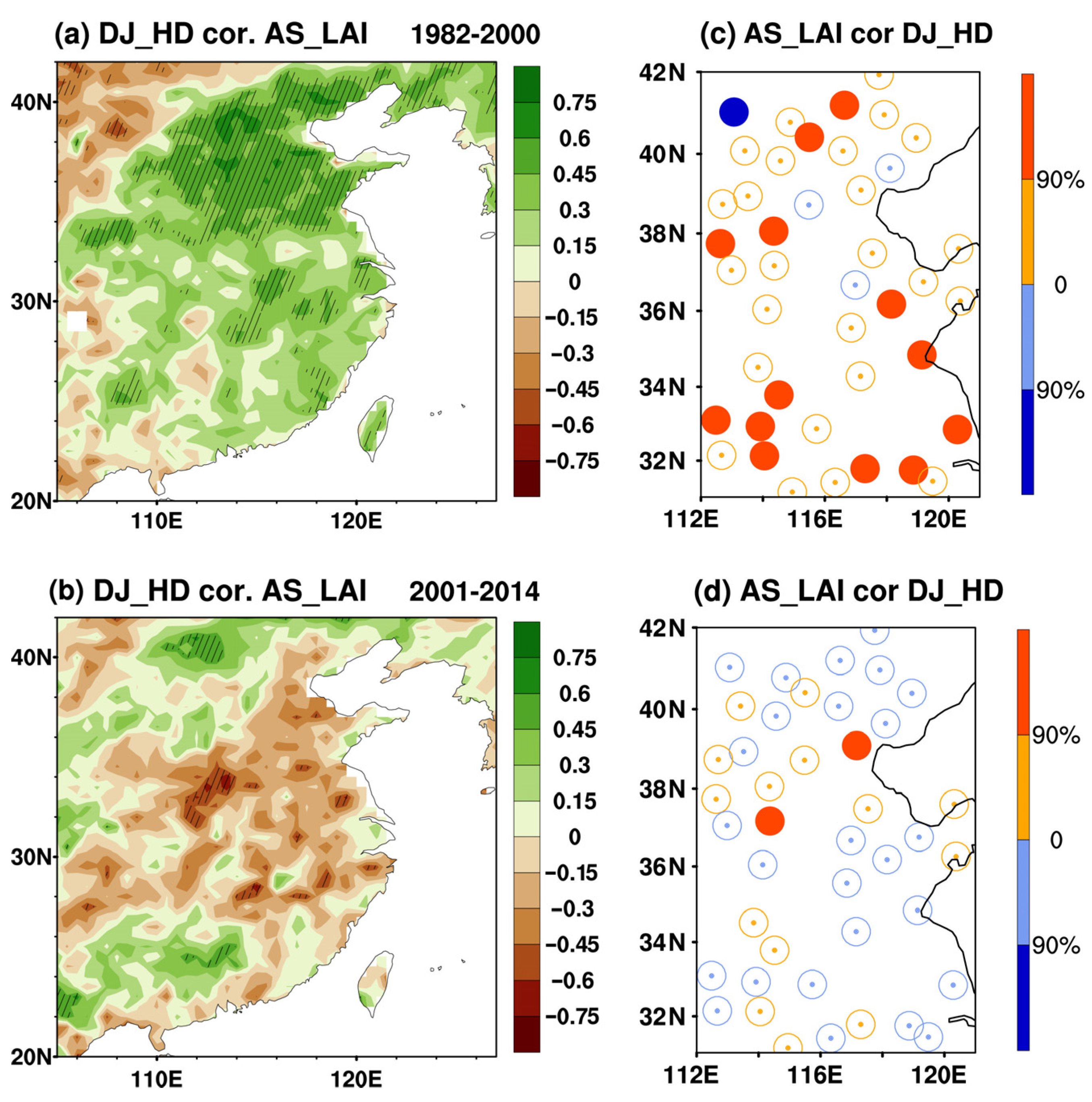
3.2. Relationships between December–January Haze Days and LAI

Monthly correlation analyses show significant correlations between DJ_HD and AS_LAI in both LAI datasets in central North China (31°–42°N, 112°–121°E; figure not shown). Figure 4a shows the time series of DJ_HD and AS_LAI based on the GLASS LAI dataset from 1982 to 2014, both of which exhibit strong interannual variabilities. Meanwhile, it appears that their variations are relatively more in-phase before 2000, whereas the opposite is the case after 2001, which is more out-of-phase. The correlations of the time series are 0.20 for the entire period; 0.71 during 1982–2000 (hereafter referred to as P1), exceeding the 99% significant level; and −0.16 during 2001–2014 (hereafter referred to as P2), which is not statistically significant. Here, we calculate the 13-year sliding correlation coefficients between DJ_HD and AS_LAI based on the GLASS LAI product. As shown in Figure 4b, the correlations are stronger and statistically significant before 2001, meaning that higher-than-normal LAI in August–September is associated with more frequent haze days during P1 and vice versa. However, this relationship is not significant in P2. Based on the LAI3g product, the correlations are 0.12 for the entire period, 0.45 during P1 (90% significant level), and −0.30 during P2 (insignificant; Figure 4c). Moreover, the 13-year sliding correlation coefficients show a sharp decrease in the correlation coefficient around the year 2000, though less significant (Figure 4d).
Figure 5a,b show the correlation coefficients and significance levels of DJ_HD index and AS_LAI at each grid point during P1 and P2, respectively. During P1, LAI anomalies in large parts of central North China show a strong in-phase relationship with DJ_HD, which is statistically significant at the 90% level. In contrast, during P2, barely scattered significant negative correlations are found in central North China. Further, the correlations between AS_LAI index and DJ_HD at each station in central North China are calculated during P1 and P2 (Figure 5c,d), from which we can see that widespread, significant positive correlations only appear during P1. On average, the LAI in central North China shows high values in August and September (Figure 6a). Meanwhile, the monthly correlations show their highest values in August and September throughout the year during 1982–2000 (Figure 6b). Thus, we speculate that AS_LAI has played an important role in the interannual variability of DJ_HD during 1982–2000 but has an insignificant relationship in 2001–2014. The correlation results are similar but less significant based on the LAI3g dataset (Figure 7). Considering the relatively clearer relationships between LAI and haze days based on the GLASS LAI product, subsequent discussion of results in the rest of this paper is related to the GLASS LAI product.

3.3. Possible Physical Mechanisms for the Significant Relationship during 1982–2000 (P1)

3.3.1. Winter Climatic Anomalies Related to December–January Haze Days during 1982–2000 (P1)

One of the most important winter climatic systems for haze is the East Asian winter monsoon [60]. Studies have revealed that a weak East Asian winter monsoon corresponds to anomalous southerly wind in the middle and lower troposphere, which is favorable for haze concentrating in eastern China [15]. The horizontal dispersion of winter haze is mostly dominated by the near-surface and low-level wind, and the vertical dispersion is affected by the vertical instabilities [61]. Thus, during a weak East Asian winter monsoon, the reduction in surface wind velocity and vertical shear of horizontal wind in the middle and lower troposphere that weakens the synoptic disturbances and vertical mixing of the atmosphere is conducive to the maintenance and development of haze [62].
Therefore, firstly, we analyze the climatic anomalies associated with high haze days so that we can proceed with the following analyses of how the August–September LAI affect these key climatic anomalies and, in turn, affect the December–January haze days. Based on the criterion that the normalized DJ_HD index is larger than 0.5 or less than −0.5 times the standard deviation, the high DJ_HD years and low DJ_HD years are selected in the composite analyses. Figure 8 illustrates the averaged winter climatic anomalies including the 850-hPa wind, 2-m temperature, 10-m wind, and boundary layer height in the high DJ_HD years minus those in low DJ_HD years, which indicate the climatic anomalies associated with high haze days. In December–January, frequent haze days are significantly associated with southerly and southeasterly wind, higher near-surface 2-m air temperature, lower near-surface 10-m wind speed, and lower boundary layer height in central North China (Figure 8). It is noted that these anomalies correspond to a weaker East Asian winter monsoon, which is consistent with previous findings [60,63]. Further, we composited the anomalies of these winter climatic factors in extreme AS_LAI years (high minus low AS_LAI years, Figure 9), and the results are similar to those in extreme DJ_HD years with the weakened East Asian winter monsoon pattern. More specifically, AS_LAI corresponds to significant southerly and southeasterly wind anomalies, positive near-surface 2-m air temperature anomalies, negative near-surface 10-m wind speed anomalies, and negative boundary layer height anomalies. Therefore, in the next section, we focus on how LAI in August–September is related to the winter climate.

3.3.2. Possible Physical Mechanisms during 1982–2000 (P1)

Figure 10 shows the evaporation anomalies associated with AS_LAI based on the linear regression coefficients and significance levels at each grid point. There are three primary components of the total near-surface evaporation, namely, vegetation transpiration, soil evaporation, and canopy evaporation [64]. Among them, vegetation transpiration indicates the root extraction, meaning the amount of water extracted from the soil. The Global Soil Wetness Project 2 estimated that vegetation transpiration and soil evaporation account for 84% of total evaporation; so, we focus on these two components [65]. Note that the downward evaporation fluxes are positive. Therefore, negative values indicate evaporation and positive values indicate condensation [57]. In August–September, soil evaporation is significantly high, and transpiration is higher in parts of central North China corresponding to higher AS_LAI (Figure 10a,b). There is an in-phase relationship between LAI and evaporation at surface (including vegetation transpiration and soil evaporation) over central North China (Figure 10c). The evaporation anomalies in association with high AS_LAI persist until October–November (Figure 10d–f). Note that vegetation transpiration is anomalously high, meaning that the amount of water extracted from the soil is high. Figure 11a shows that the volumetric soil water over most parts south of 40°N in October–November is lower in association with high AS_LAI. Previous studies have revealed that more vegetation boosts the consumption of water, causing the depletion of soil water [66,67], which is consistent with our analyses.
In general, soil water anomalies can last for months. Specifically, the “memory” of the topsoil water is about 2.5 month-long in northern China [68]. This long-term memory makes it a valuable factor for climate anomalies. Figure 11b shows that soil water anomalies in central North China have good persistence from October–November to December–January. Meanwhile, the volumetric soil water in December–January is less in central North China, corresponding to high AS_LAI (Figure 11c). Liu et al. [69] indicated that although frozen soil occurs in December–January in central North China, the surface sensible and latent heat flux anomalies can still persist from October–November to December–January—that is, the occurrence of frozen soil does not interrupt the persistence of surface heat fluxes. In this study, it is noted that the sensible heat anomalies are significantly negative and that the latent heat anomalies are positive in central North China but negative in northern and western parts in October–November (Figure 12a,b; note that the downward heat fluxes are positive; so, negative values indicate that the land surface heats the air). When the near-surface soil dries as a result of transpiration and vegetation becomes water-stressed, stomata tend to close in order to conserve the remaining water, meaning that a larger fraction of the net radiation is realized as sensible heat flux [70]. After that, in December–January, there is less downward sensible heat flux and more downward surface latent heat flux corresponding to high AS_LAI (Figure 12c,d). Meanwhile, the Qnet is calculated and shows positive anomalies, which means the land surface in central North China is likely heated owing to the drier soil corresponding to high AS_LAI (Figure 12e). Thus, Figure 12f shows higher soil temperature in the top layer.
Research has shown that the thermal condition of the land surface plays an important role in regulating the development of the East Asian monsoon [71]. The abnormally dry soil and high soil temperature in the eastern part of China narrows the land–sea temperature difference through reduced surface air temperatures [72] and weakens the East Asian winter monsoon (Figure 13). Therefore, the climatic responses of the December–January volumetric soil water (abbreviated as SW; the index is calculated based on the area-averaged (31°–38°N, 112°–120°E) value) are given in Figure 13, and the SW index is multiplied by −1 for a clear comparison. In association with lower SW, the downward surface latent heat flux increases, the downward sensible heat flux decreases, and, in turn, soil temperature increase significantly in December–January (Figure 13a–c). Meanwhile, there are easterly wind anomalies over central North China, and the boundary layer height and near-surface 10-m wind speed decrease significantly (Figure 13d–f), consistent with previous findings [73]. Note that the climatic anomalies also correspond to a weaker East Asian winter monsoon, which is favorable for the accumulation of haze particles. Therefore, the possible physical processes involved might include higher-than-normal land-surface soil temperature weakening the monsoonal circulation, which is one of the most important systems for winter haze events.
In addition to the process of evaporation, it is known that by altering the surface albedo and through partitioning of the net radiation into sensible and latent heat, vegetation has a significant impact on local and global climate [74]. Climate model experiments have shown that high vegetation cover decreases the land-surface albedo and warms the surface [75]. Figure 14 shows low surface albedo in August–November and high surface downward net solar radiation anomalies corresponding to the increased AS_LAI. The albedo anomalies may be associated with the local temperature through modulation of the incoming solar radiation, which in turn corresponds to the thermal responses in Figure 12 together with soil water anomalies. The possible physical processes may include the decreased albedo and increased surface net solar radiation boosting the land-surface heating in October–November and, thus, contributing to higher soil temperatures and anomalous surface heat fluxes, which persist to December–January and affect the monsoonal circulation for the diffusion of haze particles (Figure 12 and Figure 13).
Meanwhile, anomalies in some abnormal AS_LAI years are analyzed. For example, in 1991, DJ_HD is highest during P1 (Figure 4). The October–January volumetric soil water anomalies are negative, which correspond to higher soil temperatures, southeasterly winds, and lower 10-m wind speed anomalies in December–January (Figure 15). These anomalies all correspond to the increased AS_LAI in 1991.
It can be concluded that the anomalous soil water and surface heat fluxes corresponding to high AS_LAI may act as the bridge between August–September and December–January climatic conditions, which tends to weaken the winter monsoonal circulation and is favorable for the accumulation of haze events.

3.4. Possible Reasons for the Insignificant Relationship during 2001–2014 (P2)

During P2, the relationship between AS_LAI and soil moisture is not significant in October–November or December–January (Figure 16), which indicates that AS_LAI may not be able to impact DJ_HD through effects on soil water. Meanwhile, the significant effects of AS_LAI on the surface albedo and net solar radiation do not exist in August–September or October–November during P2 (figure not shown). As a result, the soil temperature corresponds insignificantly to AS_LAI anomalies in October–November and December–January during P2 (Figure 16). The December–January climatic anomalies corresponding to AS_LAI show insignificant patterns of the East Asian winter monsoon, including insignificant 850-hPa wind and 10-m wind speed (Figure 16)—that is, the atmospheric circulations associated with AS_LAI are not significantly linked with the ventilation conditions over central North China. Therefore, we speculate that the insignificant relationship between AS_LAI and DJ_HD during P2 might be due to the insignificant effect of AS_LAI on the ventilation conditions of haze events related to the East Asian winter monsoon.
Studies have indicated that the East Asian winter monsoon has shown decadal variations in recent decades [76]. Wang and Chen [77] suggested that the East Asian winter monsoon was amplified in the mid-2000s, and they also found that Arctic sea-ice concentration was probably responsible for this strengthening. Huang et al. [78] pointed out that the East Asian winter monsoon strengthened in the late 1990s; further, they discussed the internal dynamical causes and physical mechanism of this interdecadal variability of the East Asian winter monsoon from the dynamical theories of the Arctic Oscillation and quasi-stationary planetary wave activity. This means that, as the dominant atmospheric circulation system of haze events, the East Asian winter monsoon is likely strengthened during P2 and tends to be more significantly affected by factors including Arctic sea ice, Arctic Oscillation, quasi-stationary planetary wave activity, etc. Therefore, the effects of AS_LAI on it may become insignificant, and, in turn, the relationship between AS_LAI and DJ_HD becomes insignificant during P2.
During P2, the relationships are not significant between AS_LAI and volumetric soil water; surface soil temperature during October–January; or, in turn, the ventilation conditions of haze events related to the East Asian winter monsoon during December–January. The East Asian winter monsoon is likely strengthened during P2 and tends to be more significantly affected by factors including the Arctic sea ice, Arctic Oscillation, etc.; therefore, the effects of AS_LAI on it may become insignificant, and consequently, the relationship between AS_LAI and DJ_HD becomes insignificant during P2.

4. Discussion

Haze pollution in central North China has become a hot topic in recent decades. Relevant physical and chemical processes were investigated, and stagnant weather conditions and high anthropogenic emissions were found to play dominant roles in haze events [79,80,81]. In addition to changes in large-scale circulation revealed in previous studies, land–atmosphere interactions have also been suggested to substantially modulate haze pollution in China [35,36,82]. Therefore, this study reveals the varied relationship between LAI in August–September (AS_LAI) and haze days in December–January (DJ_HD) and the associated physical mechanisms.
In this work, the interannual relationship between DJ_HD and AS_LAI and the possible physical mechanism involved in central North China is investigated. It is found that the relationship varies in different periods, being significant during 1982–2000 (P1) but insignificant during 2001–2014 (P2). Then, the possible physical mechanisms for the significant relationship during P1 are analyzed, which is summarized in Figure 17. In August–September, there is an in-phase relationship between LAI and surface evaporation. The surface evaporation anomalies in association with high AS_LAI persist to October–November, and the amount of water extracted from the soil is high. Thus, the volumetric soil water in October–November is smaller in association with high AS_LAI. Meanwhile, low surface albedo in August–November and high surface downward net solar radiation anomalies corresponding to the increased AS_LAI work together with the evaporation processes, and their thermal responses are reflected in significant heat flux anomalies and higher surface soil temperatures in October–November. In turn, both the volumetric soil water and heat flux anomalies persist to December–January, which corresponds to an anomalous winter climate associated with haze events, including easterly wind anomalies, lower boundary layer height, and decreased near-surface 10-m wind speed over central North China. However, during P2, the relationships are not significant between AS_LAI and evaporation or surface albedo in October–January, which, in turn, corresponds to insignificant soil water and soil temperature anomalies during October–January. The December–January climatic anomalies corresponding to AS_LAI show insignificant patterns of the East Asian winter monsoon, which are also not significantly linked with the ventilation conditions of haze events over central North China. Meanwhile, the East Asian winter monsoon is likely strengthened during P2 and tends to be more significantly affected by factors including the Arctic sea ice, Arctic Oscillation, etc. Therefore, the effects of AS_LAI on the East Asian winter monsoon may become insignificant, and, in turn, the relationship between AS_LAI and DJ_HD becomes insignificant during P2.
At present in meteorological studies, statistical analyses and climate dynamics diagnoses are still important tools to reveal the physical processes and mechanisms among climate variables. Based on multiple sets of data including observational haze data, satellite-based LAI data, meteorological reanalysis data, and so on, this work reveals that variations in previous LAIs are related to December to January haze days over central North China. Systematic climate dynamic analyses are carried out including multivariate empirical orthogonal function, 13-year-sliding correlation, linear regression, multiyear composite analyses, and typical case analysis to diagnose this relationship—that is, the detailed diagnoses of meteorological variables related to DJ_HD and AS_LAI, as well as the key dynamical and thermal processes involved, to reveal the possible physical mechanisms of their relationship. Therefore, we found that the variations of LAI, ahead of variations of haze days, are valuable to the prediction of haze days and can be used as an efficient predictor. On the other hand, limited by the simulation abilities of climate models for describing vegetation annual variations, efforts will be made to try more suitable models and to conduct more investigations in numerical model experiments designed for the verification of our data by analyzing results in our future work. Some studies have simulated haze events using numerical modelling [24,83], and our results provide the observational base for numerical studies. Moreover, in addition to the biophysical effects of vegetation, it is known that from the biochemical perspective vegetation provides an important source for haze pollution through the formation of secondary organic aerosols—that is, biogenic volatile organic compounds [46,47]. The cooperative biophysical–biochemical effect is still an open question that needs to be answered. Another question that deserves more discussion is why the relationship shifted around the year 2000 and why the relationships among AS_LAI, soil water, and soil temperature become insignificant during October–January. The questions mentioned above will be addressed in our group’s future work. Moreover, based on the previously revealed mechanisms, efforts have been made to predict haze pollution by using both numerical and statistical models [84,85]. The results were encouraging but there is still room for improvement [23]. Therefore, the significant relationship of LAI and haze days revealed in this work is likely to have the potential to improve the prediction skill of haze pollution in central North China, which can be considered in prediction models and help decision-making for pollutants control in the future.

Author Contributions

Conceptualization, K.F.; methodology, K.F. and L.J.; software, L.J.; validation, L.J.; formal analysis, L.J.; investigation, L.J.; resources, K.F.; data curation, L.J.; writing—original draft preparation, L.J.; writing—review and editing, K.F.; visualization, L.J.; supervision, K.F.; project administration, K.F.; funding acquisition, K.F. All authors have read and agreed to the published version of the manuscript.

Funding

This research was funded by the National Natural Science Foundation of China (NSFC) (grant numbers 42088101 and 41730964) and the Innovation Group Project of the Southern Marine Science and Engineering Guangdong Laboratory (Zhuhai) (grant number 311021001).

Institutional Review Board Statement

Not applicable.

Informed Consent Statement

Not applicable.

Data Availability Statement

The GSOD database is available at https://www.ncei.noaa.gov/access/metadata/landing-page/bin/iso?id=gov.noaa.ncdc:C00516 (accessed on 16 December 2021). The GLASS LAI product is available at http://www.glass.umd.edu/introduction.html (accessed on 16 December 2021). ERA5 data are available at https://cds.climate.copernicus.eu/cdsapp#!/home (accessed on 16 December 2021). Surface albedo data are available at https://wui.cmsaf.eu/safira/action/viewICDRDetails?acronym=CLARA_AVHRR_V002_ICDR (accessed on 16 December 2021).

Acknowledgments

The authors are grateful to the editors and anonymous reviewers. This research was jointly supported by the National Natural Science Foundation of China (grant numbers 42088101 and 41730964) and the Innovation Group Project of the Southern Marine Science and Engineering Guangdong Laboratory (Zhuhai) (grant number 311021001).

Conflicts of Interest

The authors declare no conflict of interest.

References

  1. Watson, J.G. Visibility: Science and Regulation. J. Air Waste Manag. 2002, 52, 628–713. [Google Scholar] [CrossRef] [Green Version]
  2. Zhang, X.Y.; Sun, J.Y.; Wang, Y.Q.; Li, W.J.; Zhang, Q.; Wang, W.G.; Quan, J.N.; Cao, G.L.; Wang, J.Z.; Yang, Y.Q.; et al. Factors contributing to haze and fog in China. Chin. Sci. Bull. 2013, 58, 1178–1187. [Google Scholar] [CrossRef]
  3. Lelieveld, J.; Evans, J.S.; Fnais, M.; Giannadaki, D.; Pozzer, A. The contribution of outdoor air pollution sources to premature mortality on a global scale. Nature 2015, 525, 367–371. [Google Scholar] [CrossRef] [PubMed]
  4. Li, J.; Sun, J.; Zhou, M.; Cheng, Z.; Li, Q.; Cao, X.; Zhang, J. Observational analyses of dramatic developments of a severe air pollution event in the Beijing area. Atmos. Chem. Phys. 2018, 18, 3919–3935. [Google Scholar] [CrossRef] [Green Version]
  5. Ramanathan, V.; Crutzen, P.J.; Kiehl, J.T.; Rosenfeld, D. Aerosols, Climate, and the Hydrological Cycle. Science 2001, 294, 2119–2124. [Google Scholar] [CrossRef] [PubMed] [Green Version]
  6. Wang, T.J.; Zhuang, B.L.; Li, S.; Liu, J.; Xie, M.; Yin, C.Q.; Zhang, Y.; Yuan, C.; Zhu, J.L.; Ji, L.Q.; et al. The interactions between anthropogenic aerosols and the East Asian summer monsoon using RegCCMS. J. Geophys. Res. Atmos. 2015, 120, 5602–5621. [Google Scholar] [CrossRef]
  7. Wang, Y.H.; Liu, Z.R.; Zhang, J.K.; Hu, B.; Ji, D.S.; Yu, Y.C.; Wang, Y.S. Aerosol physicochemical properties and implications for visibility during an intense haze episode during winter in Beijing. Atmos. Chem. Phys. 2015, 15, 3205–3215. [Google Scholar] [CrossRef] [Green Version]
  8. Cohen, A.J.; Brauer, M.; Burnett, R.; Anderson, H.R.; Frostad, J.; Estep, K.; Balakrishnan, K.; Brunekreef, B.; Dandona, L.; Dandona, R.; et al. Estimates and 25-year trends of the global burden of disease attributable to ambient air pollution: An analysis of data from the Global Burden of Diseases Study 2015. Lancet 2017, 389, 1907–1918. [Google Scholar] [CrossRef] [Green Version]
  9. Zhang, Q.; Jiang, X.; Tong, D.; Davis, S.J.; Zhao, H.; Geng, G.; Feng, T.; Zheng, B.; Lu, Z.; Streets, D.G.; et al. Transboundary health impacts of transported global air pollution and international trade. Nature 2017, 543, 705–709. [Google Scholar] [CrossRef] [Green Version]
  10. Gao, M.; Guttikunda, S.K.; Carmichael, G.R.; Wang, Y.; Liu, Z.; Stanier, C.O.; Saide, P.E.; Yu, M. Health impacts and economic losses assessment of the 2013 severe haze event in Beijing area. Sci. Total Environ. 2015, 511, 553–561. [Google Scholar] [CrossRef]
  11. Cleaner air for China. Nat. Geosci. 2019, 12, 497. [CrossRef]
  12. Cai, W.; Li, K.; Liao, H.; Wang, H.; Wu, L. Weather conditions conducive to Beijing severe haze more frequent under climate change. Nat. Clim. Chang. 2017, 7, 257–262. [Google Scholar] [CrossRef]
  13. Zhu, W.; Xu, X.; Zheng, J.; Yan, P.; Wang, Y.; Cai, W. The characteristics of abnormal wintertime pollution events in the Jing-Jin-Ji region and its relationships with meteorological factors. Sci. Total Environ. 2018, 626, 887–898. [Google Scholar] [CrossRef]
  14. Duan, F.K.; He, K.B.; Ma, Y.L.; Yang, F.M.; Yu, X.C.; Cadle, S.H.; Chan, T.; Mulawa, P.A. Concentration and chemical characteristics of PM2.5 in Beijing, China: 2001–2002. Sci. Total Environ. 2006, 355, 264–275. [Google Scholar] [CrossRef]
  15. Zhang, R.; Li, Q.; Zhang, R. Meteorological conditions for the persistent severe fog and haze event over eastern China in January 2013. Sci. China Earth Sci. 2014, 57, 26–35. [Google Scholar] [CrossRef]
  16. Wang, Y.; Yao, L.; Wang, L.; Liu, Z.; Ji, D.; Tang, G.; Zhang, J.; Sun, Y.; Hu, B.; Xin, J. Mechanism for the formation of the January 2013 heavy haze pollution episode over central and eastern China. Sci. China Earth Sci. 2014, 57, 14–25. [Google Scholar] [CrossRef]
  17. Li, K.; Liao, H.; Cai, W.; Yang, Y. Attribution of Anthropogenic Influence on Atmospheric Patterns Conducive to Recent Most Severe Haze Over Eastern China. Geophys. Res. Lett. 2018, 45, 2072–2081. [Google Scholar] [CrossRef]
  18. Sun, Y.; Jiang, Q.; Wang, Z.; Fu, P.; Li, J.; Yang, T.; Yin, Y. Investigation of the sources and evolution processes of severe haze pollution in Beijing in January 2013. J. Geophys. Res. Atmos. 2014, 119, 4380–4398. [Google Scholar] [CrossRef]
  19. Zhang, Z.; Wang, J.; Chen, L.; Chen, X.; Sun, G.; Zhong, N.; Kan, H.; Lu, W. Impact of haze and air pollution-related hazards on hospital admissions in Guangzhou, China. Environ. Sci. Pollut. Res. 2014, 21, 4236–4244. [Google Scholar] [CrossRef]
  20. Wang, X.; Wei, W.; Cheng, S.; Li, J.; Zhang, H.; Lv, Z. Characteristics and classification of PM2.5 pollution episodes in Beijing from 2013 to 2015. Sci. Total Environ. 2018, 612, 170–179. [Google Scholar] [CrossRef]
  21. Chen, H.; Wang, H. Haze Days in North China and the associated atmospheric circulations based on daily visibility data from 1960 to 2012. J. Geophys. Res. Atmos. 2015, 120, 5895–5909. [Google Scholar] [CrossRef]
  22. Wang, H.J.; Chen, H.P.; Liu, J.P. Arctic Sea Ice Decline Intensified Haze Pollution in Eastern China. Atmos. Ocean. Sci. Lett. 2015, 8, 1–9. [Google Scholar] [CrossRef]
  23. Yin, Z.; Zhou, B.; Chen, H.; Li, Y. Synergetic impacts of precursory climate drivers on interannual-decadal variations in haze pollution in North China: A review. Sci. Total Environ. 2021, 755, 143017. [Google Scholar] [CrossRef] [PubMed]
  24. Dang, R.; Liao, H. Severe winter haze days in the Beijing–Tianjin–Hebei region from 1985 to 2017 and the roles of anthropogenic emissions and meteorology. Atmos. Chem. Phys. 2019, 19, 10801–10816. [Google Scholar] [CrossRef] [Green Version]
  25. Huang, K.; Zhuang, G.; Lin, Y.; Fu, J.S.; Wang, Q.; Liu, T.; Zhang, R.; Jiang, Y.; Deng, C.; Fu, Q.; et al. Typical types and formation mechanisms of haze in an Eastern Asia megacity, Shanghai. Atmos. Chem. Phys. 2012, 12, 105–124. [Google Scholar] [CrossRef] [Green Version]
  26. Hao, J.; Tian, H.; Lu, Y. Emission Inventories of NOx from Commercial Energy Consumption in China, 1995−1998. Environ. Sci. Technol. 2002, 36, 552–560. [Google Scholar] [CrossRef]
  27. Wang, H.-J.; Chen, H.-P. Understanding the recent trend of haze pollution in eastern China: Roles of climate change. Atmos. Chem. Phys. 2016, 16, 4205–4211. [Google Scholar] [CrossRef] [Green Version]
  28. Yang, Y.; Liao, H.; Lou, S. Increase in winter haze over eastern China in recent decades: Roles of variations in meteorological parameters and anthropogenic emissions. J. Geophys. Res. Atmos. 2016, 121, 13050–13065. [Google Scholar] [CrossRef] [Green Version]
  29. He, C.; Liu, R.; Wang, X.; Liu, S.C.; Zhou, T.; Liao, W. How does El Niño-Southern Oscillation modulate the interannual variability of winter haze days over eastern China? Sci. Total Environ. 2019, 651, 1892–1902. [Google Scholar] [CrossRef] [Green Version]
  30. Liu, T.; Gong, S.; He, J.; Yu, M.; Wang, Q.; Li, H.; Liu, W.; Zhang, J.; Li, L.; Wang, X.; et al. Attributions of meteorological and emission factors to the 2015 winter severe haze pollution episodes in China’s Jing-Jin-Ji area. Atmos. Chem. Phys. 2017, 17, 2971–2980. [Google Scholar] [CrossRef] [Green Version]
  31. Wu, P.; Ding, Y.; Liu, Y. Atmospheric circulation and dynamic mechanism for persistent haze events in the Beijing–Tianjin–Hebei region. Adv. Atmos. Sci. 2017, 34, 429–440. [Google Scholar] [CrossRef] [Green Version]
  32. Jia, B.; Wang, Y.; Yao, Y.; Xie, Y. A new indicator on the impact of large-scale circulation on wintertime particulate matter pollution over China. Atmos. Chem. Phys. 2015, 15, 11919–11929. [Google Scholar] [CrossRef] [Green Version]
  33. Yang, Q.; Yuan, D. Central North Pacific SST anomalies linked late winter haze to Arctic sea ice. Int. J. Climatol. 2020, 40, 5542–5555. [Google Scholar] [CrossRef]
  34. Zhao, S.; Li, J.; Sun, C. Decadal variability in the occurrence of wintertime haze in central eastern China tied to the Pacific Decadal Oscillation. Sci. Rep. 2016, 6, 27424. [Google Scholar] [CrossRef] [PubMed]
  35. Zhang, Y.; Yin, Z.; Wang, H. Roles of climate variability on the rapid increases of early winter haze pollution in North China after 2010. Atmos. Chem. Phys. 2020, 20, 12211–12221. [Google Scholar] [CrossRef]
  36. Yin, Z.; Wang, H. The strengthening relationship between Eurasian snow cover and December haze days in central North China after the mid-1990s. Atmos. Chem. Phys. 2018, 18, 4753–4763. [Google Scholar] [CrossRef] [Green Version]
  37. McPherson, R.A. A review of vegetation—Atmosphere interactions and their influences on mesoscale phenomena. Prog. Phys. Geogr. Earth Environ. 2007, 31, 261–285. [Google Scholar] [CrossRef]
  38. Taylor, C.M.; Lebel, T. Observational evidence of persistent convective-scale rainfall patterns. Mon. Weather Rev. 1998, 126, 1597–1607. [Google Scholar] [CrossRef]
  39. Cox, P.M.; Betts, R.A.; Jones, C.D.; Spall, S.A.; Totterdell, I.J. Acceleration of global warming due to carbon-cycle feedbacks in a coupled climate model. Nature 2000, 408, 184–187. [Google Scholar] [CrossRef]
  40. Alkama, R.; Cescatti, A. Biophysical climate impacts of recent changes in global forest cover. Science 2016, 351, 600–604. [Google Scholar] [CrossRef] [Green Version]
  41. Duveiller, G.; Hooker, J.; Cescatti, A. The mark of vegetation change on Earth’s surface energy balance. Nat. Commun. 2018, 9, 679. [Google Scholar] [CrossRef] [Green Version]
  42. Zhao, K.; Jackson, R.B. Biophysical forcings of land-use changes from potential forestry activities in North America. Ecol. Monogr. 2014, 84, 329–353. [Google Scholar] [CrossRef]
  43. Duo, A.; Zhao, W.; Qu, X.; Jing, R.; Xiong, K. Spatio-temporal variation of vegetation coverage and its response to climate change in North China plain in the last 33 years. Int. J. Appl. Earth Obs. 2016, 53, 103–117. [Google Scholar] [CrossRef]
  44. Gong, Z.; Zhao, S.; Gu, J. Correlation analysis between vegetation coverage and climate drought conditions in North China during 2001–2013. J. Geogr. Sci. 2017, 27, 143–160. [Google Scholar] [CrossRef]
  45. Liu, Z.Y.; Notaro, M.; Kutzbach, J.; Liu, N. Assessing global vegetation-climate feedbacks from observations. J. Clim. 2006, 19, 787–814. [Google Scholar] [CrossRef]
  46. Chang, J.; Ren, Y.; Shi, Y.; Zhu, Y.; Ge, Y.; Hong, S.; Jiao, L.; Lin, F.; Peng, C.; Mochizuki, T.; et al. An inventory of biogenic volatile organic compounds for a subtropical urban–rural complex. Atmos. Environ. 2012, 56, 115–123. [Google Scholar] [CrossRef]
  47. Guenther, A.; Hewitt, C.N.; Erickson, D.; Fall, R.; Geron, C.; Graedel, T.; Harley, P.; Klinger, L.; Lerdau, M.; Mckay, W.A.; et al. A global model of natural volatile organic compound emissions. J. Geophys. Res. Atmos. 1995, 100, 8873–8892. [Google Scholar] [CrossRef]
  48. Kaufmann, R.K.; Zhou, L.; Myneni, R.B.; Tucker, C.J.; Slayback, D.; Shabanov, N.V.; Pinzon, J. The effect of vegetation on surface temperature: A statistical analysis of NDVI and climate data. Geophys. Res. Lett. 2003, 30, 2147. [Google Scholar] [CrossRef] [Green Version]
  49. Bonan, G.B.; Pollard, D.; Thompson, S.L. Effects of boreal forest vegetation on global climate. Nature 1992, 359, 716. [Google Scholar] [CrossRef]
  50. Ding, Y.; Liu, Y. Analysis of long-term variations of fog and haze in China in recent 50 years and their relations with atmospheric humidity. Sci. China Earth Sci. 2014, 57, 36–46. [Google Scholar] [CrossRef]
  51. Schichtel, B.A.; Husar, R.B.; Falke, S.R.; Wilson, W.E. Haze trends over the United States, 1980–1995. Atmos. Environ. 2001, 35, 5205–5210. [Google Scholar] [CrossRef]
  52. Yin, Z.; Wang, H.; Chen, H. Understanding severe winter haze events in the North China Plain in 2014: Roles of climate anomalies. Atmos. Chem. Phys. 2017, 17, 1641–1651. [Google Scholar] [CrossRef] [Green Version]
  53. Doyle, M.; Dorling, S. Visibility trends in the UK 1950–1997. Atmos. Environ. 2002, 36, 3161–3172. [Google Scholar] [CrossRef]
  54. Li, S.; Han, Z.; Chen, H. A comparison of the effects of interannual Arctic sea ice loss and ENSO on winter haze days: Observational analyses and AGCM simulations. J. Meteorol. Res. 2017, 31, 820–833. [Google Scholar] [CrossRef]
  55. Xiao, Z.; Liang, S.; Wang, J.; Xiang, Y.; Zhao, X.; Song, J. Long-Time-Series Global Land Surface Satellite Leaf Area Index Product Derived From MODIS and AVHRR Surface Reflectance. IEEE Trans. Geosci. Remote 2016, 54, 5301–5318. [Google Scholar] [CrossRef]
  56. Zhu, Z.; Bi, J.; Pan, Y.; Ganguly, S.; Anav, A.; Xu, L.; Samanta, A.; Piao, S.; Nemani, R.; Myneni, R. Global Data Sets of Vegetation Leaf Area Index (LAI)3g and Fraction of Photosynthetically Active Radiation (FPAR)3g Derived from Global Inventory Modeling and Mapping Studies (GIMMS) Normalized Difference Vegetation Index (NDVI3g) for the Period 1981 to 2011. Remote Sens. 2013, 5, 927. [Google Scholar]
  57. Hersbach, H.; Bell, B.; Berrisford, P.; Hirahara, S.; Horányi, A.; Muñoz-Sabater, J.; Nicolas, J.; Peubey, C.; Radu, R.; Schepers, D.; et al. The ERA5 global reanalysis. Q. J. R. Meteorol. Soc. 2020, 146, 1999–2049. [Google Scholar] [CrossRef]
  58. Karlsson, K.-G.; Riihelä, A.; Trentmann, J.; Stengel, M.; Meirink, J.F.; Solodovnik, I.; Devasthale, A.; Manninen, T.; Jääskeläinen, E.; Anttila, K.; et al. ICDR AVHRR—Based on CLARA-A2 Methods, Satellite Application Facility on Climate Monitoring. 2021. Available online: https://wui.cmsaf.eu/safira/action/viewICDRDetails?acronym=CLARA_AVHRR_V002_ICDR (accessed on 17 December 2021).
  59. Wang, B. The vertical structure and development of the ENSO anomaly mode during 1979-89. J. Atmos. Sci. 1992, 49, 698–712. [Google Scholar] [CrossRef] [Green Version]
  60. Li, Q.; Zhang, R.; Wang, Y. Interannual variation of the wintertime fog–haze days across central and eastern China and its relation with East Asian winter monsoon. Int. J. Climatol. 2016, 36, 346–354. [Google Scholar] [CrossRef]
  61. Yin, Z.; Wang, H. Role of atmospheric circulations in haze pollution in December 2016. Atmos. Chem. Phys. 2017, 17, 11673–11681. [Google Scholar] [CrossRef] [Green Version]
  62. Xu, X.; Zhao, T.; Liu, F.; Gong, S.L.; Kristovich, D.; Lu, C.; Guo, Y.; Cheng, X.; Wang, Y.; Ding, G. Climate modulation of the Tibetan Plateau on haze in China. Atmos. Chem. Phys. 2016, 16, 1365–1375. [Google Scholar] [CrossRef] [Green Version]
  63. Liu, Q.; Sheng, L.; Cao, Z.; Diao, Y.; Wang, W.; Zhou, Y. Dual effects of the winter monsoon on haze-fog variations in eastern China. J. Geophys. Res. Atmos. 2017, 122, 5857–5869. [Google Scholar] [CrossRef]
  64. Lawrence, D.M.; Slingo, J.M. An annual cycle of vegetation in a GCM. Part I: Implementation and impact on evaporation. Clim. Dyn. 2004, 22, 87–105. [Google Scholar] [CrossRef]
  65. Lawrence, D.M.; Thornton, P.E.; Oleson, K.W.; Bonan, G.B. The Partitioning of Evapotranspiration into Transpiration, Soil Evaporation, and Canopy Evaporation in a GCM: Impacts on Land–Atmosphere Interaction. J. Hydrometeorol. 2007, 8, 862–880. [Google Scholar] [CrossRef]
  66. Pielke Sr, R.A.; Avissar, R.; Raupach, M.; Dolman, A.J.; Zeng, X.; Denning, A.S. Interactions between the atmosphere and terrestrial ecosystems: Influence on weather and climate. Glob. Chang. Biol. 1998, 4, 461–475. [Google Scholar] [CrossRef]
  67. Wang, W.; Anderson, B.T.; Entekhabi, D.; Huang, D.; Kaufmann, R.K.; Potter, C.; Myneni, R.B. Feedbacks of Vegetation on Summertime Climate Variability over the North American Grasslands. Part II: A Coupled Stochastic Model. Earth Interact. 2006, 10, 1–30. [Google Scholar] [CrossRef] [Green Version]
  68. Entin, J.K.; Robock, A.; Vinnikov, K.Y.; Hollinger, S.E.; Liu, S.; Namkhai, A. Temporal and spatial scales of observed soil moisture variations in the extratropics. J. Geophys. Res.-Atmos. 2000, 105, 11865–11877. [Google Scholar] [CrossRef]
  69. Liu, L.; Zhang, R.; Zuo, Z. The Relationship between Soil Moisture and LAI in Different Types of Soil in Central Eastern China. J. Hydrometeorol. 2016, 17, 2733–2742. [Google Scholar] [CrossRef]
  70. Avissar, R.; Pielke, R.A. The impact of plant stomatal control on mesoscale atmospheric circulations. Agric. For. Meteorol. 1991, 54, 353–372. [Google Scholar] [CrossRef]
  71. Xue, Y.; Juang, H.-M.H.; Li, W.-P.; Prince, S.; DeFries, R.; Jiao, Y.; Vasic, R. Role of land surface processes in monsoon development: East Asia and West Africa. J. Geophys. Res. Atmos. 2004, 109, D03105. [Google Scholar] [CrossRef]
  72. Zhang, R.; Zuo, Z. Impact of Spring Soil Moisture on Surface Energy Balance and Summer Monsoon Circulation over East Asia and Precipitation in East China. J. Clim. 2011, 24, 3309–3322. [Google Scholar] [CrossRef]
  73. Liu, G.; Chen, J.-M.; Ji, L.-R.; Sun, S.-Q. Relationship of summer soil moisture with early winter monsoon and air temperature over eastern China. Int. J. Climatol. 2012, 32, 1513–1519. [Google Scholar] [CrossRef]
  74. Bonan, G.B.; Chapin, F.S.; Thompson, S.L. Boreal forest and tundra ecosystems as components of the climate system. Clim. Chang. 1995, 29, 145–167. [Google Scholar] [CrossRef]
  75. Dickinson, R.E.; Hanson, B. Vegetation-Albedo Feedbacks. In Climate Processes and Climate Sensitivity; Wiley: Hoboken, NJ, USA, 1984; pp. 180–186. [Google Scholar] [CrossRef]
  76. Miao, J.; Wang, T. Decadal variations of the East Asian winter monsoon in recent decades. Atmos. Sci. Lett. 2020, 21, e960. [Google Scholar] [CrossRef] [Green Version]
  77. Wang, L.; Chen, W. The East Asian winter monsoon: Re-amplification in the mid-2000s. Chin. Sci. Bull. 2014, 59, 430–436. [Google Scholar] [CrossRef]
  78. Huang, R.; Liu, Y.; Huangfu, J.; Feng, T. Characteristics and Internal Dynamical Causes of the Interdecadal Variability of East Asian Winter Monsoon near the Late 1990s. Chin. J. Atmos. Sci. 2014, 38, 627–644. [Google Scholar]
  79. Li, J.; Du, H.; Wang, Z.; Sun, Y.; Yang, W.; Li, J.; Tang, X.; Fu, P. Rapid formation of a severe regional winter haze episode over a mega-city cluster on the North China Plain. Environ. Pollut. 2017, 223, 605–615. [Google Scholar] [CrossRef]
  80. Zhao, X.J.; Zhao, P.S.; Xu, J.; Meng, W.; Pu, W.W.; Dong, F.; He, D.; Shi, Q.F. Analysis of a winter regional haze event and its formation mechanism in the North China Plain. Atmos. Chem. Phys. 2013, 13, 5685–5696. [Google Scholar] [CrossRef] [Green Version]
  81. Liu, X.G.; Li, J.; Qu, Y.; Han, T.; Hou, L.; Gu, J.; Chen, C.; Yang, Y.; Liu, X.; Yang, T.; et al. Formation and evolution mechanism of regional haze: A case study in the megacity Beijing, China. Atmos. Chem. Phys. 2013, 13, 4501–4514. [Google Scholar] [CrossRef] [Green Version]
  82. Zou, Y.; Wang, Y.; Zhang, Y.; Koo, J.-H. Arctic sea ice, Eurasia snow, and extreme winter haze in China. Sci. Adv. 2017, 3, e1602751. [Google Scholar] [CrossRef] [Green Version]
  83. Zhang, L.; Wang, T.; Lv, M.; Zhang, Q. On the severe haze in Beijing during January 2013: Unraveling the effects of meteorological anomalies with WRF-Chem. Atmos. Environ. 2015, 104, 11–21. [Google Scholar] [CrossRef]
  84. Yin, Z.; Wang, H. Seasonal prediction of winter haze days in the north central North China Plain. Atmos. Chem. Phys. 2016, 16, 14843–14852. [Google Scholar] [CrossRef] [Green Version]
  85. Yin, Z.; Wang, H. Statistical Prediction of Winter Haze Days in the North China Plain Using the Generalized Additive Model. J. Appl. Meteorol. Climatol. 2017, 56, 2411–2419. [Google Scholar] [CrossRef]
Figure 1. (a) Climatology of total haze days throughout a year at 119 meteorological stations in eastern China during 1980–2018 (unit: days); (b) the monthly area-averaged haze days at each station over eastern China during 1980–2018 (unit: days).
Remotesensing 14 00884 g001
Figure 2. Climatology of total haze days in (a) December and (b) January at 119 meteorological stations in eastern China during 1980–2018 (unit: days).
Remotesensing 14 00884 g002
Figure 3. First spatial mode of the MV-EOF of the (a) December and (b) January haze days at 42 meteorological stations in central North China; (c) the corresponding time series during 1980–2018. The variance explained by the EOF mode is shown above the right-hand corner in (c).
Remotesensing 14 00884 g003
Figure 4. Time series of normalized area-averaged DJ_HD (blue bars) and (a) AS_LAI (marked lines, GLASS dataset) and (c) AS_LAI3g (marked lines, LAI3g dataset). The 13-year-sliding correlation coefficient between area-averaged DJ_HD and (b) AS_LAI (GLASS dataset) and (d) AS_LAI3g (LAI3g dataset), where the two solid reference lines denote statistically significant correlations (α = 0.10; Student’s t-test).
Remotesensing 14 00884 g004
Figure 5. Correlation between area-averaged DJ_HD index and AS_LAI at each grid point during (a) 1982–2000 and (b) 2001–2014. Correlation between area-averaged AS_LAI index and DJ_HD at each station during (c) 1982–2000 and (d) 2001–2014. Slashes and solid dots represent significant (α = 0.10; Student’s t-test).
Remotesensing 14 00884 g005
Figure 6. (a) Monthly area-averaged LAIs over central North China and (b) their correlation coefficients with DJ_HD during 1982–2000.
Remotesensing 14 00884 g006
Figure 7. Correlation between area-averaged DJ_HD index and AS_LAI3g at each grid point during (a) 1982–2000 and (b) 2001–2014. Correlation between area-averaged AS_LAI3g index and DJ_HD at each station during (c) 1982–2000 and (d) 2001–2014. Slashes and solid dots represent significant (α = 0.10; Student’s t-test).
Remotesensing 14 00884 g007
Figure 8. Composite differences of the December–January (a) 850-hPa wind (unit: m s−1), (b) 2-m temperature (unit: K), (c) 10-m wind speed (unit: m s−1), and (d) boundary layer height (unit: m) between positive and negative DJ_HD years during 1982–2000. Shaded and slashed regions are significant (α = 0.10; Student’s t-test).
Remotesensing 14 00884 g008
Figure 9. Composite differences of the December–January (a) 850-hPa wind (unit: m s−1), (b) 2-m temperature (unit: K), (c) 10-m wind speed (unit: m s−1), and (d) boundary layer height (unit: m) between positive and negative AS_LAI years during 1982–2000. Shaded and slashed regions are significant (α = 0.10; Student’s t-test).
Remotesensing 14 00884 g009
Figure 10. Linear regression of the August–September (a) evaporation from soil (unit: mm of water equivalent), (b) evaporation from vegetation transpiration (unit: mm of water equivalent), and (c) evaporation at surface (unit: mm of water equivalent) and of the October–November (d) evaporation from soil, (e) evaporation from vegetation transpiration, and (f) evaporation at surface on AS_LAI index during 1982–2000. Slashed regions are significant (α = 0.10; Student’s t-test).
Remotesensing 14 00884 g010
Figure 11. Linear regression of the (a) October–November and (c) December–January volumetric soil water (layer: 0–7 cm; unit: m3 m−3) on AS_LAI index during 1982–2000. (b) Correlation between area-averaged October–November volumetric soil water index and December–January volumetric soil water during 1982–2000. Slashed regions are significant (α = 0.10; Student’s t-test).
Remotesensing 14 00884 g011
Figure 12. Linear regression of the October–November (a) surface sensible heat flux (unit: W m−2) and (b) surface latent heat flux (unit: W m−2), and of the December–January (c) surface sensible heat flux, (d) surface latent heat flux, (e) Qnet (unit: W m−2), and (f) soil temperature (layer: 0–7 cm; unit: K) on AS_LAI index during 1982–2000. Slashed regions are significant (α = 0.10; Student’s t-test).
Remotesensing 14 00884 g012
Figure 13. Linear regression of the December–January (a) surface latent heat flux (unit: W m−2), (b) surface sensible heat flux (unit: W m−2), (c) soil temperature (layer: 0–7 cm; unit: K), (d) 850-hPa wind (unit: m s−1), (e) boundary layer height (unit: m), and (f) 10-m wind speed (unit: m s−1) on negative December–January volumetric soil water index (layer: 0–7 cm; unit: m3 m−3; the index is multiplied by −1 for a clear comparison) during 1982–2000. Slashed and shaded regions are significant (α = 0.10; Student’s t-test).
Remotesensing 14 00884 g013
Figure 14. Linear regression of the (a) August–September and (b) October–November surface albedo (unit: %), and of the (c) October–November surface net solar radiation (unit: W m−2) on AS_LAI index during 1982–2000. Slashed regions are significant (α = 0.10; Student’s t-test).
Remotesensing 14 00884 g014
Figure 15. Anomalies of the (a) August–September LAI, (b) October–November volumetric soil water (layer: 0–7 cm; unit: m3 m−3), and of the December–January (c) volumetric soil water, (d) soil temperature (layer: 0–7 cm; unit: K), (e) 850-hPa wind (unit: m s−1), and (f) 10-m wind speed (unit: m s−1) in 1991.
Remotesensing 14 00884 g015
Figure 16. Linear regression of the October–November (a) volumetric soil water (layer: 0–7 cm; unit: m3 m−3), (b) soil temperature (layer: 0–7 cm; unit: K), and of the December–January (c) volumetric soil water (layer: 0–7 cm; unit: m3 m−3), (d) soil temperature (layer: 0–7 cm; unit: K), (e) 850-hPa wind (unit: m s−1), and (f) 10-m wind speed (unit: m s−1) on AS_LAI index during 2001–2014. Slashed and shaded regions are significant (α = 0.10; Student’s t-test).
Remotesensing 14 00884 g016
Figure 17. Possible physical mechanisms of the responses of DJ_HD to AS_LAI during P1 (SH indicates sensible heat flux anomalies; LH indicates latent heat flux anomalies).
Remotesensing 14 00884 g017
Publisher’s Note: MDPI stays neutral with regard to jurisdictional claims in published maps and institutional affiliations.

