
The Influence of Anisotropic Surface Reflection on Earth’s Outgoing Shortwave Radiance in the Lunar Direction

 , ,
, ,
Abstract
:1. Introduction
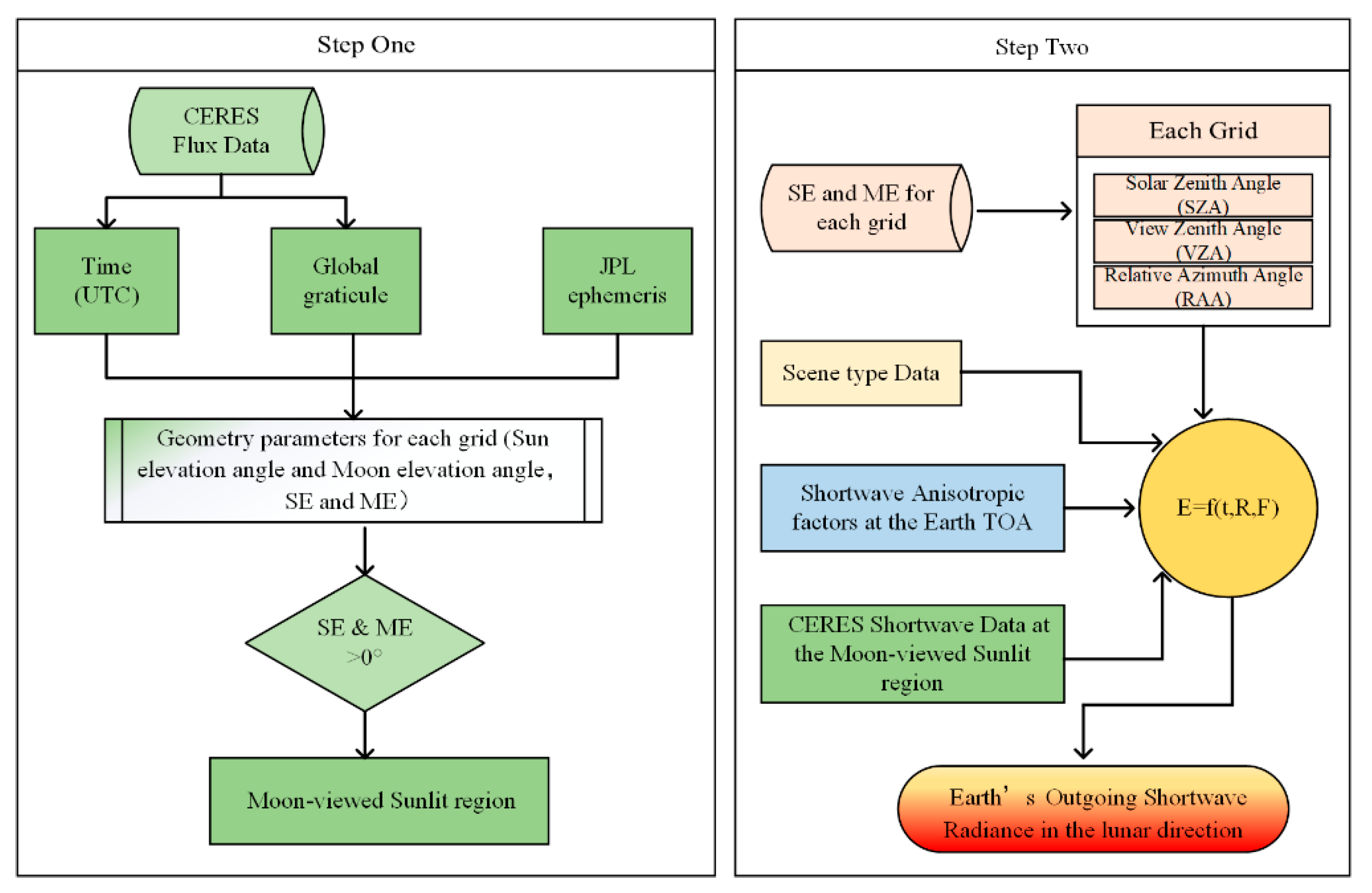
2. Methods
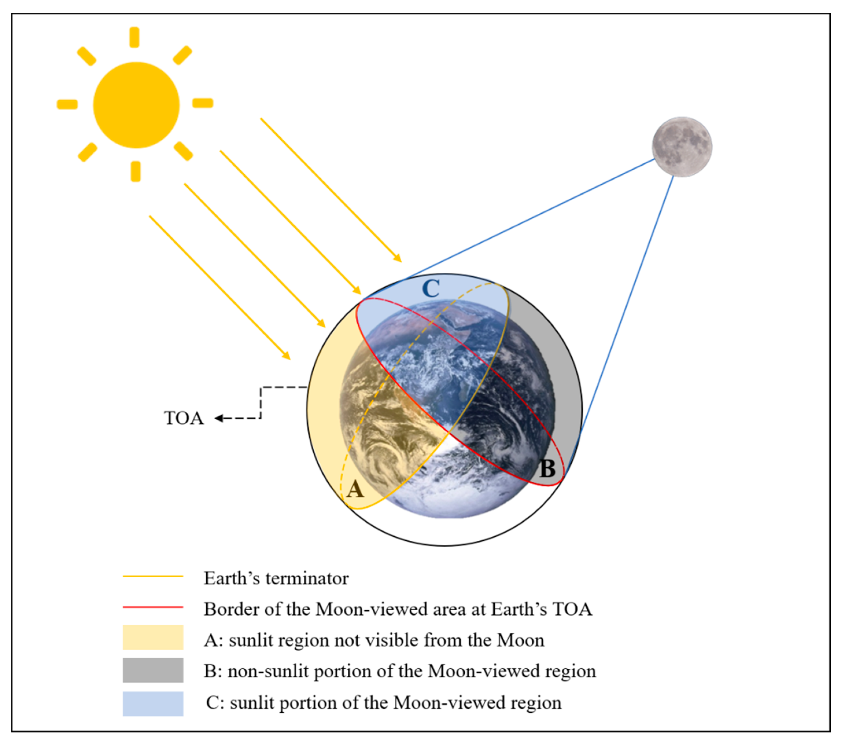
2.1. Spatiotemporal Distribution of the Moon-Viewed Sunlit Region
2.1.1. The Moon-Viewed Sunlit Region on Earth
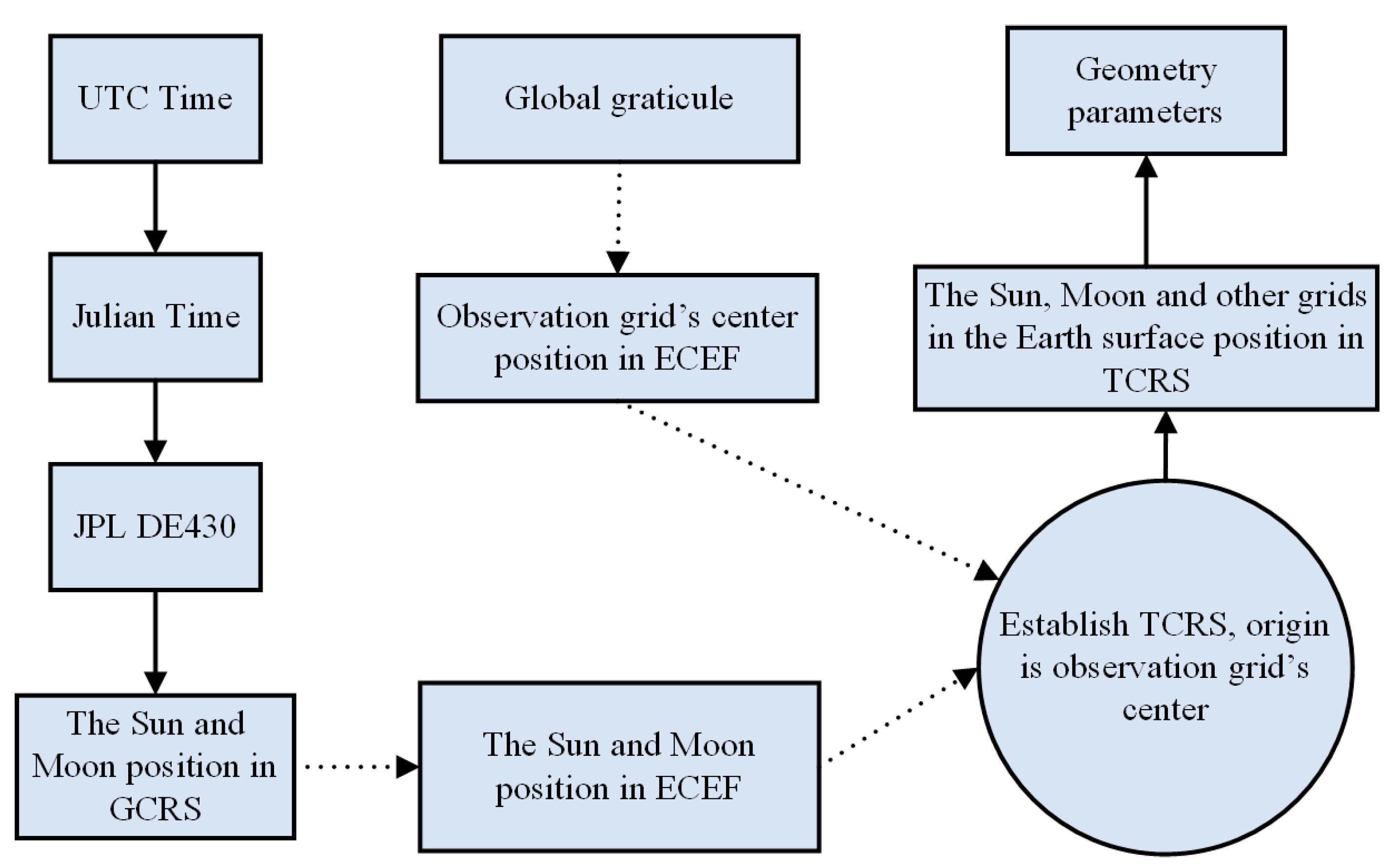
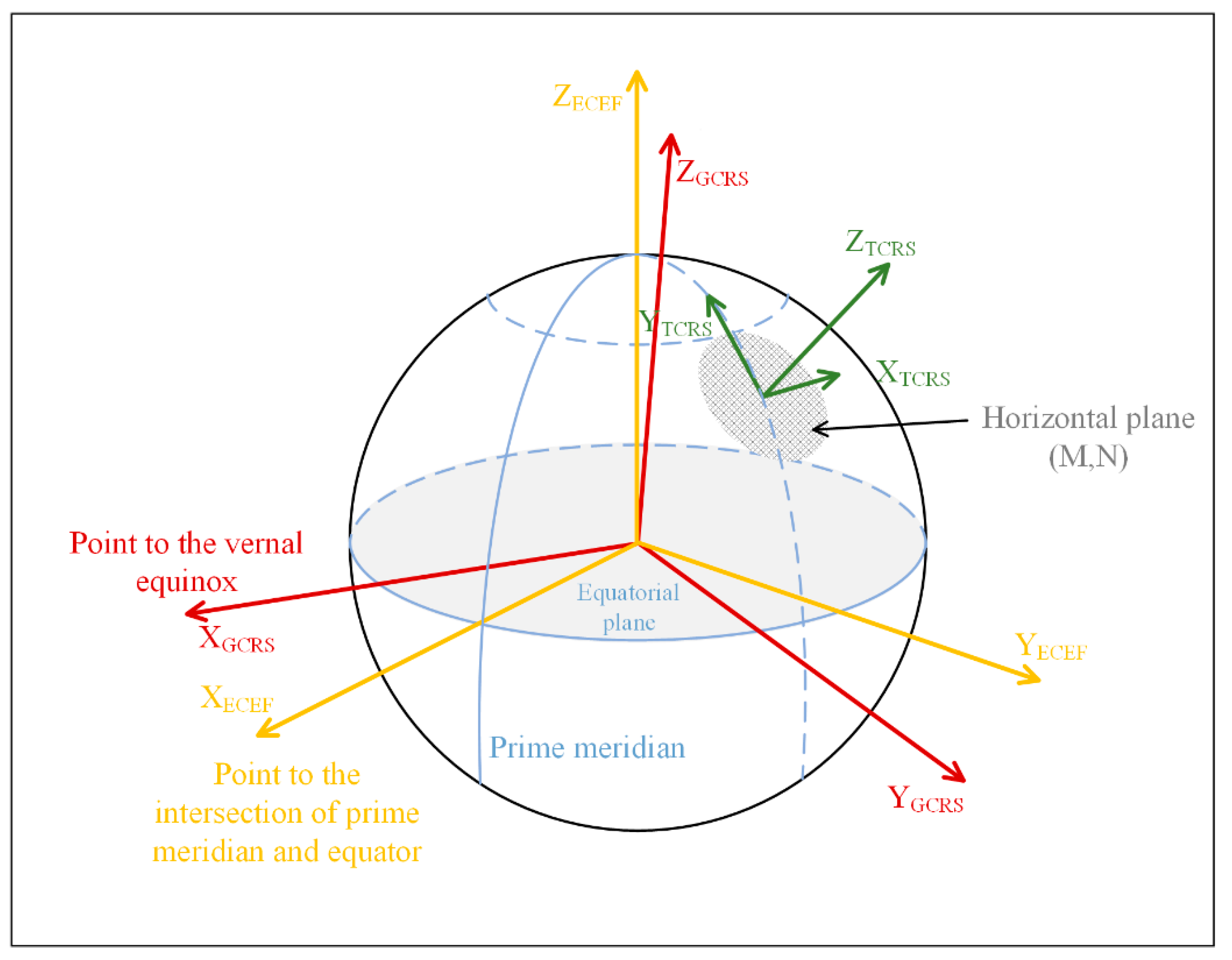
2.1.2. Transformation of the Reference Systems
2.1.3. Calculation of the Geometrical Parameters
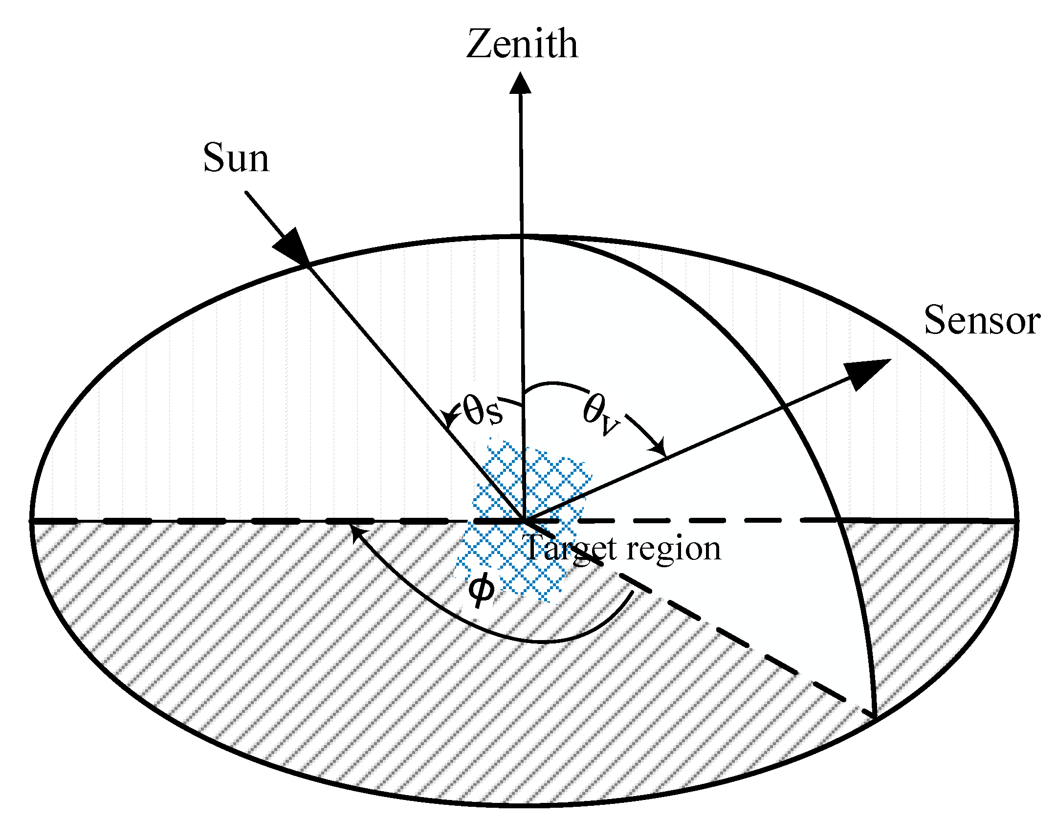
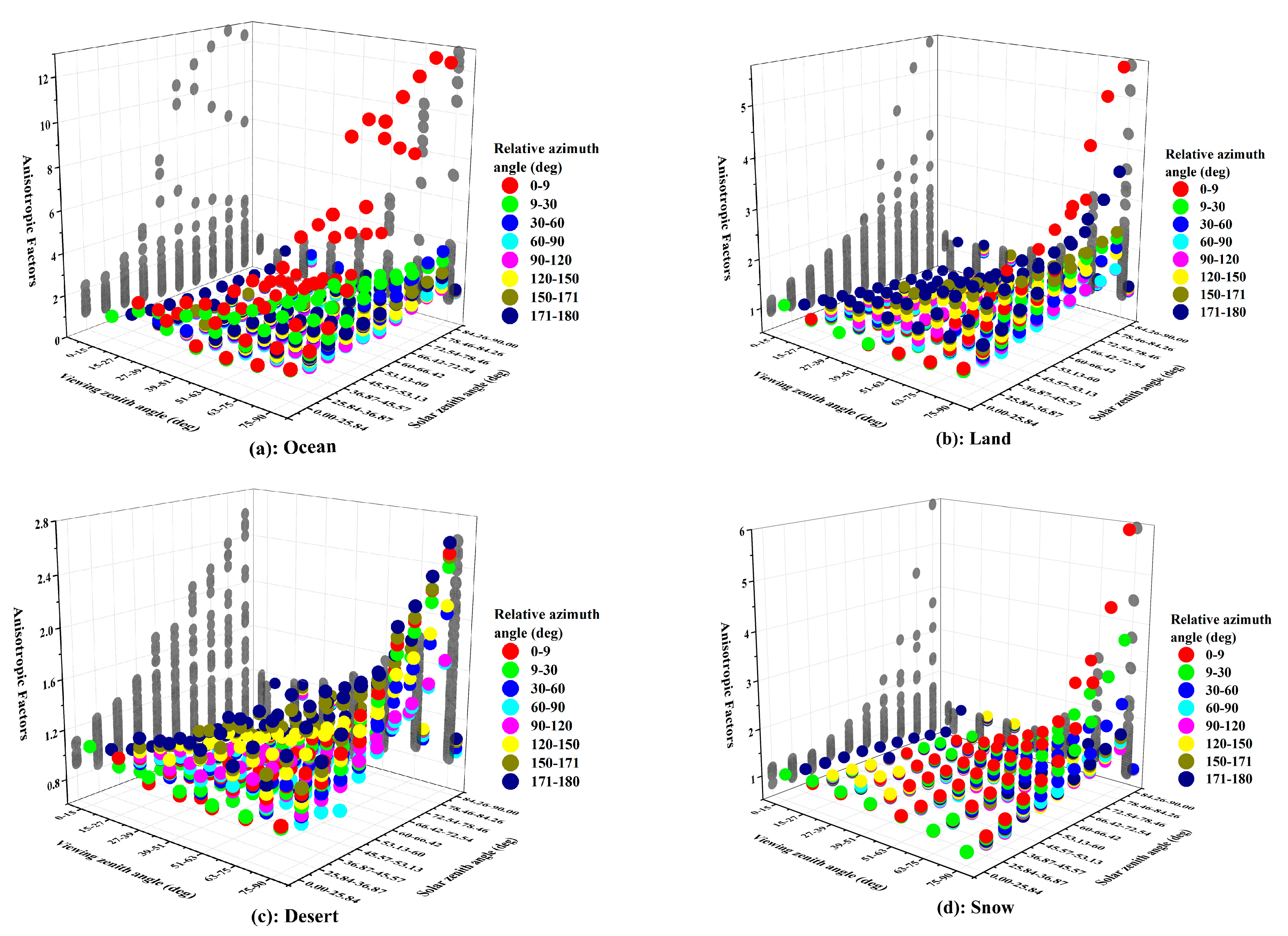
2.2. Anisotropic Factors from CERES/ERBE ADMs
2.3. Estimation of Earth’s OSR in the Lunar Direction
3. Results
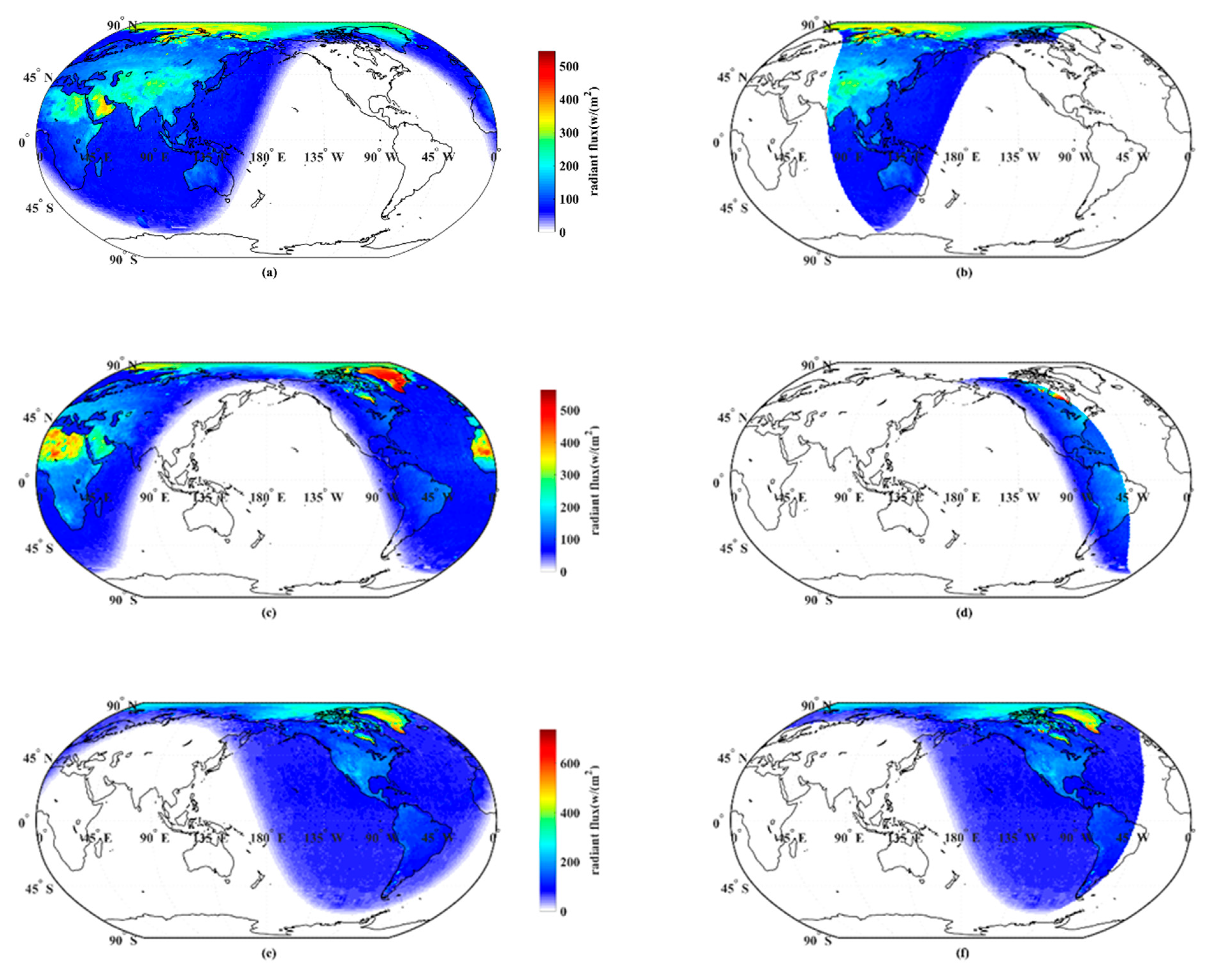
3.1. Distribution of Moon-Viewed Sunlit Region
3.2. Anisotropic EOSRiLD over Different Periods
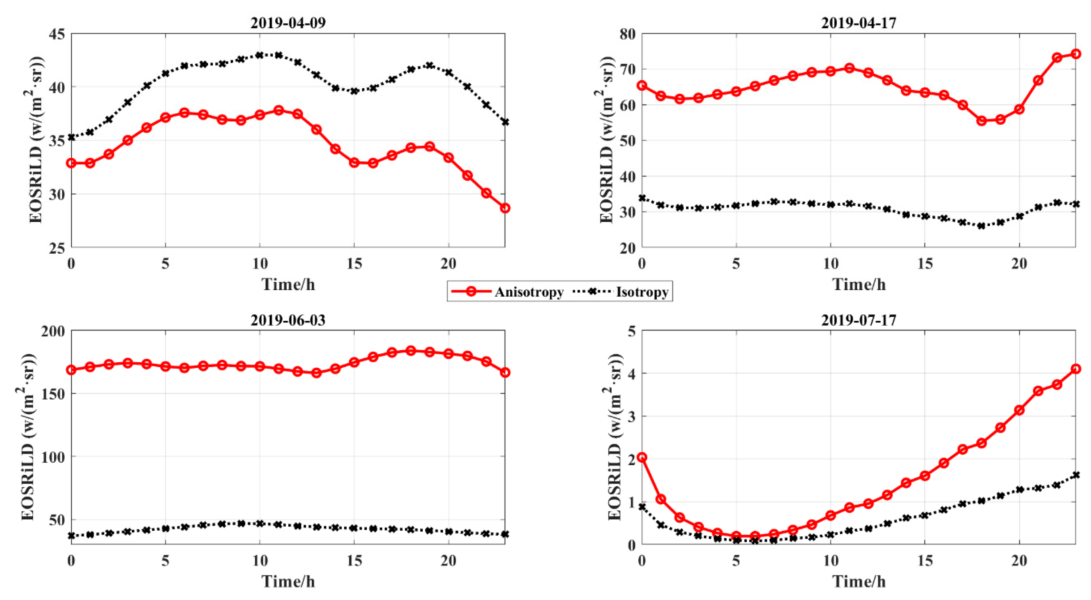
3.2.1. Anisotropic EOSRiLD over Earth’s Rotation Period
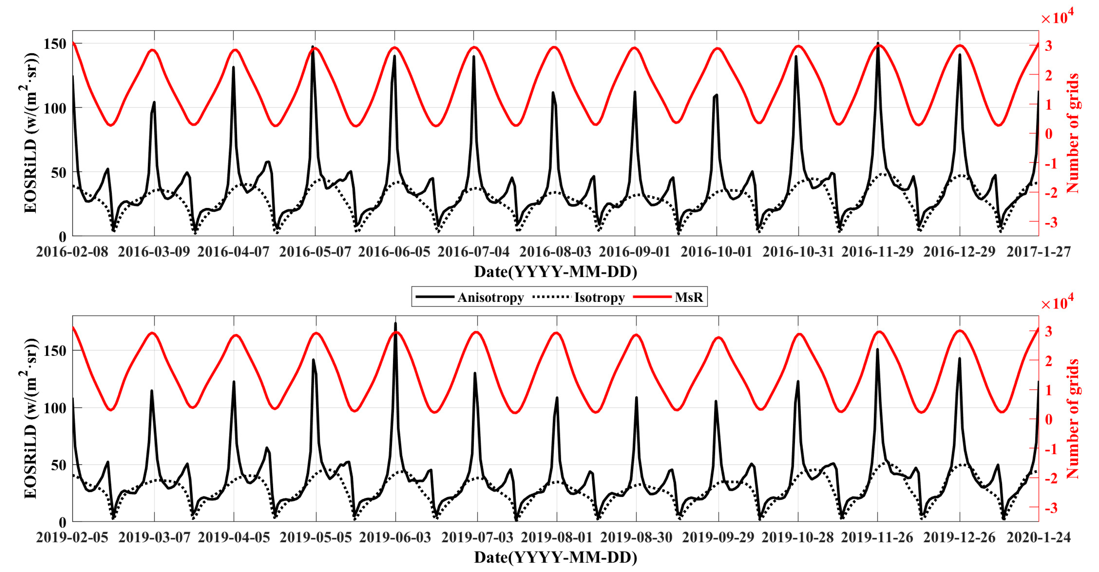
3.2.2. Anisotropic EOSRiLD over Earth’s Revolution Period
3.2.3. Anisotropic EOSRiLD over the Synodic Month Cycle
4. Discussion
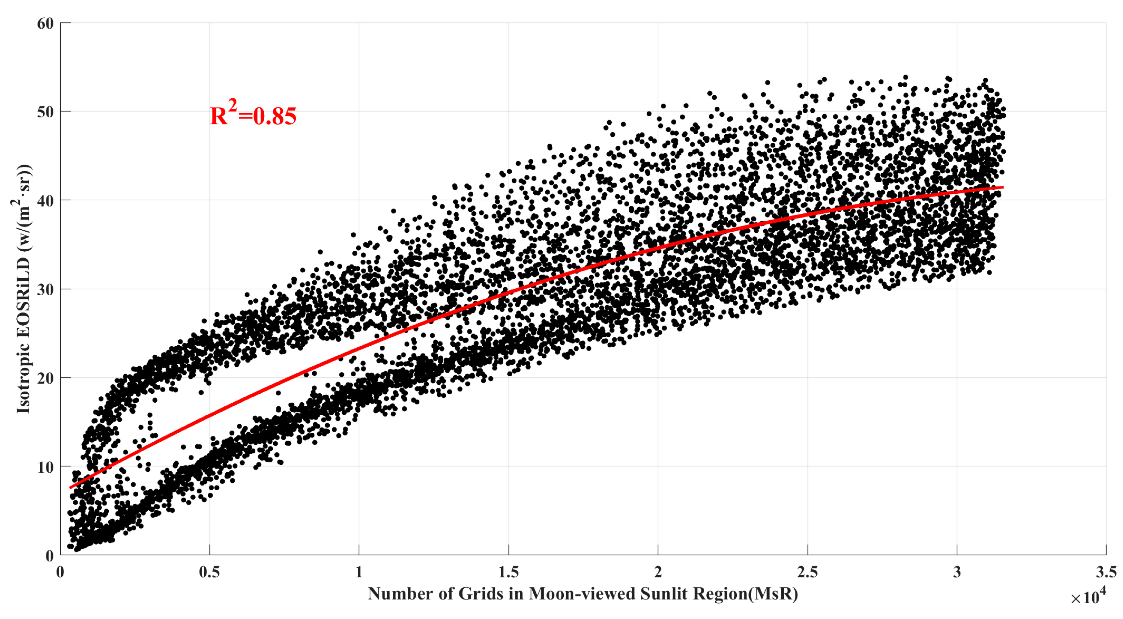
4.1. Impact of the Area of Moon-Viewed Sunlit Region on Anisotropic EOSRiLD
4.2. Impact of the Anisotropic Factors on Anisotropic EOSRiLD
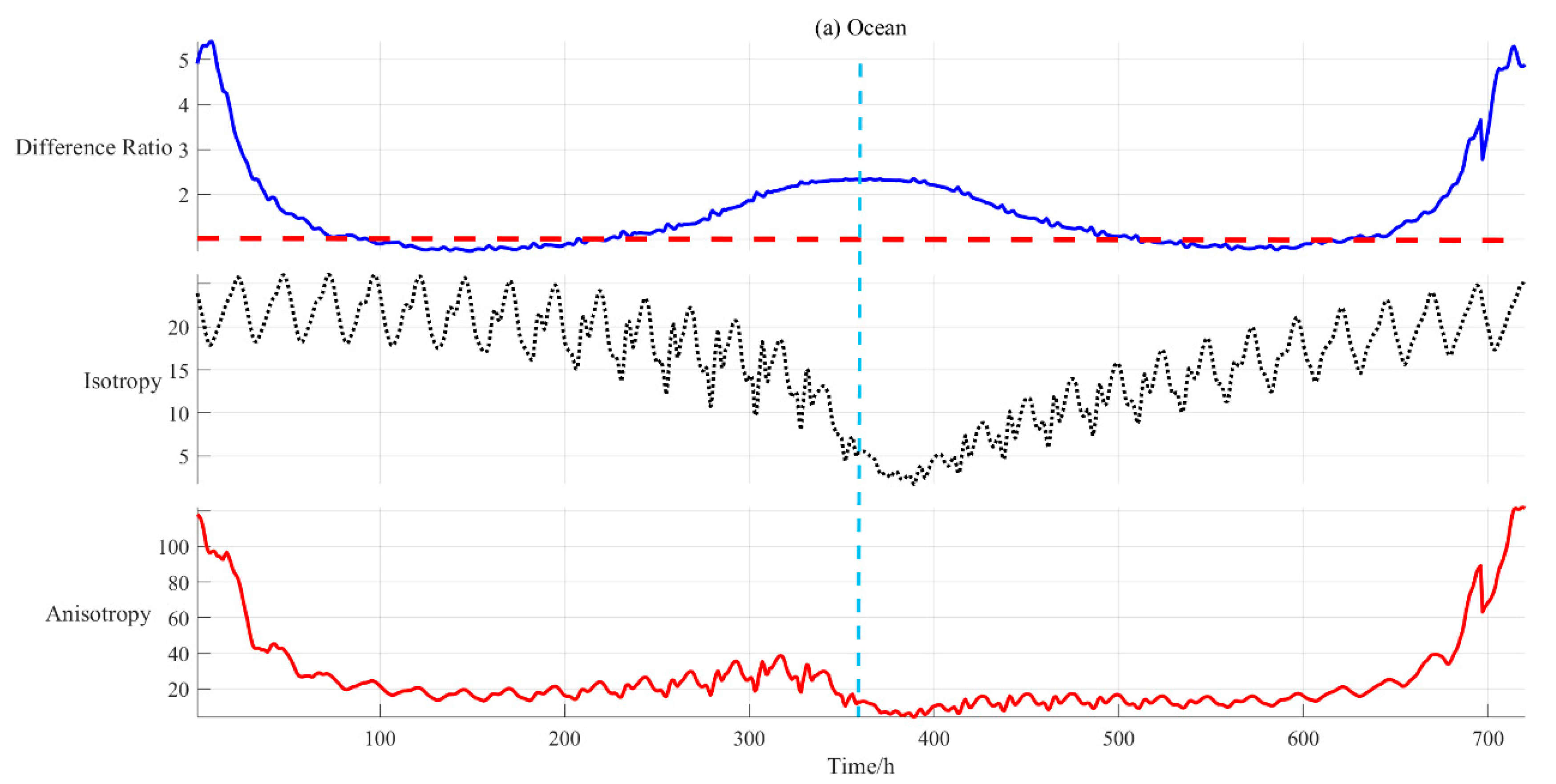
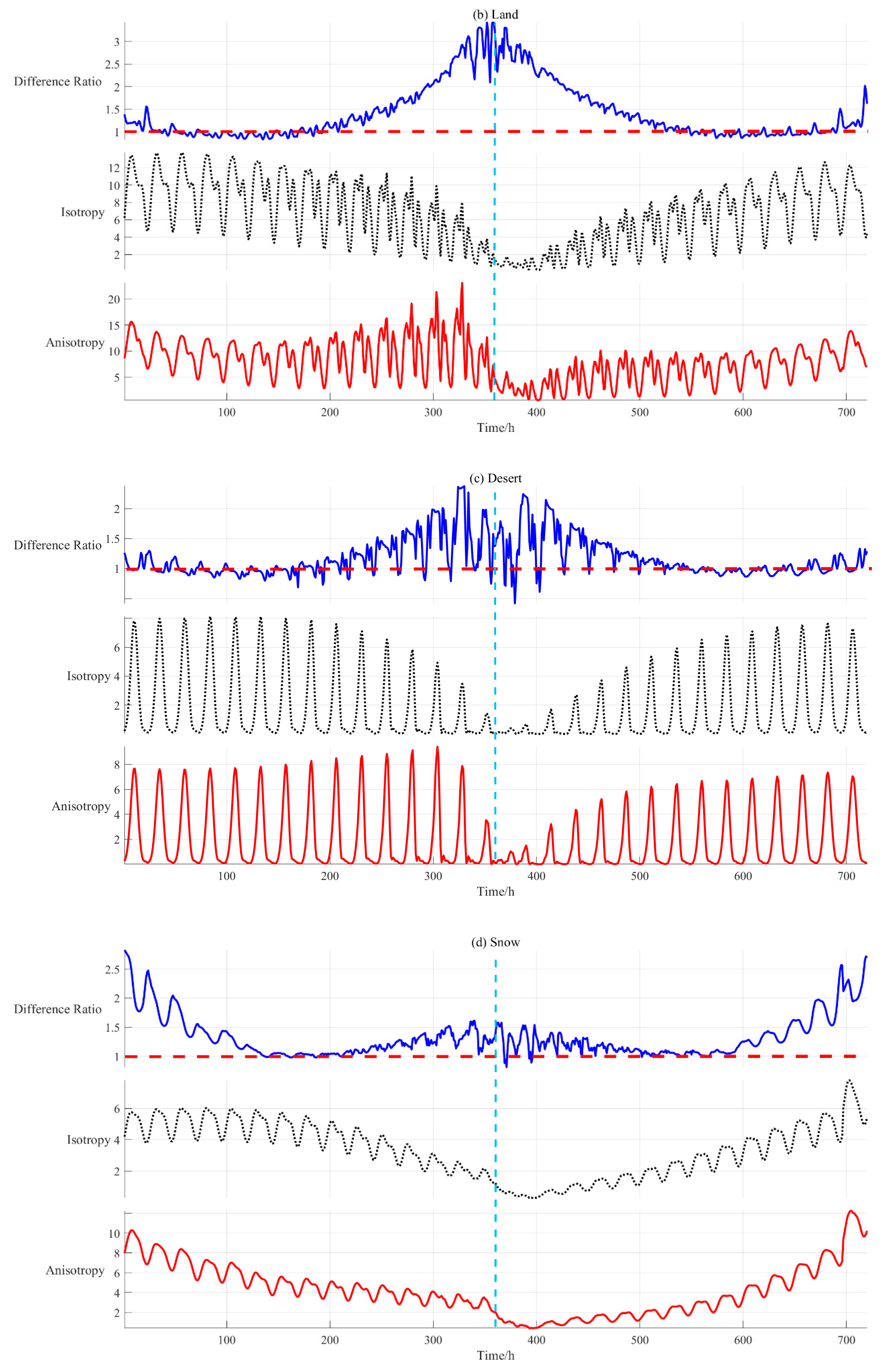
4.2.1. Impact of Scene Types on Anisotropic EOSRiLD
4.2.2. Impact of Incident-Viewing Angular Bins on Anisotropic EOSRiLD
5. Conclusions
Author Contributions
Funding
Data Availability Statement
Acknowledgments
Conflicts of Interest
Appendix A
| TOA | Top of atmosphere |
| OSR | Outgoing shortwave radiation |
| ERB | Earth radiation budget |
| MS | Moon-based Sensor |
| MsR | Moon-viewed sunlit region |
| LEO | Low-Earth orbit |
| ERBE | Earth Radiation Budget Experiment |
| CERES | Clouds and Earth’s Radiant Energy System |
| SORCE | Solar Radiation and Climate Experiment |
| GERB | Geostationary Earth Radiation Budget |
| NISTAR | National Institute of Standards and Technology Advanced Radiometer |
| DSCOVR | Deep Space Climate Observatory |
| OHC | Ocean heat capacity |
| EOSRiLD | Earth outgoing shortwave radiance in the lunar direction |
| GCRS | Geocentric Celestial Reference System |
| GCS | Geodetic Coordinate System |
| ECEF | Earth-centered Earth-fixed |
| TCRS | Topocentric Cartesian reference system |
| CCS | Cartesian coordinate system |
| EA | Elevation angle |
| ZA | Zenith angle |
| AA | Azimuth angle |
| ADM | Angular distribution model |
| RAA | Relative azimuth angle |
| MZA | Moon zenith angle |
Appendix B
- (1)
- GCRS to ECEF
- (2)
- GCS to ECEF
- (3)
- ECEF to TCRS
Appendix C

| Solar Calendar | Lunar Calendar | Solar Calendar | Lunar Calendar |
|---|---|---|---|
| 8 February 2016 | 1st day of 1st month | 8 March 2016 | Last day of 1st month |
| 5 February 2019 | 5 March 2019 | ||
| 9 March 2016 | 1st day of 2nd month | 6 April 2016 | Last day of 2nd month |
| 7 March 2019 | 4 April 2019 | ||
| 7 April 2016 | 1st day of 3rd month | 5 May 2016 | Last day of 3rd month |
| 5 April 2019 | 4 May 2019 | ||
| 6 May 2016 | 1st day of 4th month | 4 June 2016 | Last day of 4th month |
| 5 May 2019 | 2 June 2019 | ||
| 5 June 2016 | 1st day of 5th month | 3 July 2016 | Last day of 5th month |
| 3 June 2019 | 2 July 2019 | ||
| 4 July 2016 | 1st day of 6th month | 2 August 2016 | Last day of 6th month |
| 3 July 2019 | 31 July 2019 | ||
| 3 August 2016 | 1st day of 7th month | 31 August 2016 | Last day of 7th month |
| 1 August 2019 | 29 August 2019 | ||
| 1 September 2019 | 1st day of 8th month | 30 September 2016 | Last day of 8th month |
| 30 August 2019 | 28 September 2019 | ||
| 1 October 2016 | 1st day of 9th month | 30 October 2016 | Last day of 9th month |
| 29 September 2019 | 27 October 2019 | ||
| 31 October 2016 | 1st day of 10th month | 28 November 2016 | Last day of 10th month |
| 28 October 2019 | 25 November 2019 | ||
| 29 November 2016 | 1st day of 11th month | 28 December 2016 | Last day of 11th month |
| 26 November 2019 | 25 December 2019 | ||
| 29 December 2019 | 1st day of 12th month | 27 January 2017 | Last day of 12th month |
| 26 December 2019 | 24 January 2020 |
References
- Von Schuckmann, K.; Palmer, M.D.; Trenberth, K.E.; Cazenave, A.; Chambers, D.P.; Champollion, N.; Hansen, J.E.; Josey, S.A.; Loeb, N.; Mathieu, P.P. An imperative to monitor Earth’s energy imbalance. Nat. Clim. Change 2016, 6, 138–144. [Google Scholar] [CrossRef] [Green Version]
- Trenberth, K.E.; Stepaniak, D.P. Covariability of Components of Poleward Atmospheric Energy Transports on Seasonal and Interannual Timescales. J. Clim. 2003, 16, 3691–3705. [Google Scholar] [CrossRef]
- Trenberth, K.E.; Stepaniak, D.P. Seamless Poleward Atmospheric Energy Transports and Implications for the Hadley Circulation. J. Clim. 2003, 16, 3706–3722. [Google Scholar] [CrossRef]
- Trenberth, K.E.; Fasullo, J.T.; Kiehl, J. Earth’s Global Energy Budget. Bull. Am. Meteorol. Soc. 2009, 90, 311–323. [Google Scholar] [CrossRef]
- Barkstrom, B.R.; Smith, G.L. The Earth Radiation Budget Experiment: Science and implementation. Rev. Geophys. 1986, 24, 379–390. [Google Scholar] [CrossRef]
- Harries, J.; Crommelynck, D. The Geostationary Earth Radiation Budget Experiment on MSG-1 and its Potential Applications. Adv. Space Res. 1999, 24, 915–919. [Google Scholar] [CrossRef]
- Wielicki, B.A.; Barkstrom, B.R.; Harrison, E.F.; III, R.B.L.; Smith, G.L.; Cooper, J.E. Clouds and the Earth’s Radiant Energy System (CERES): An Earth Observing System Experiment. Bull. Am. Meteorol. Soc. 1996, 77, 853–868. [Google Scholar] [CrossRef] [Green Version]
- Kopia, L.P. Earth Radiation Budget Experiment Scanner Instrument. Rev. Geophys. 1986, 24, 400–406. [Google Scholar] [CrossRef]
- Luther, M.R.; Cooper, J.E.; Taylor, G.R. The Earth Radiation Budget Experiment Nonscanner Instrument (Paper 5R0789). Rev. Geophys. 1986, 24, 391–399. [Google Scholar] [CrossRef]
- Wielicki, B.A.; Barkstrom, B.R.; Baum, B.A.; Charlock, T.P.; Green, R.N.; Kratz, D.P.; Lee, R.B.; Minnis, P.; Smith, G.L.; Takmeng, W.; et al. Clouds and the Earth’s Radiant Energy System (CERES): Algorithm overview. IEEE Trans. Geosci. Remote Sens. 1998, 36, 1127–1141. [Google Scholar] [CrossRef] [Green Version]
- Rottman, G.; Woods, T.; George, V. The Solar Radiation and Climate Experiment (SORCE). Sol. Phys. 2005, 230, 360–417. [Google Scholar]
- Smith, G.L.; Wong, T.; Bush, K.A. Time-Sampling Errors of Earth Radiation From Satellites: Theory for Outgoing Longwave Radiation. IEEE Trans. Geosci. Remote Sens. 2015, 53, 1656–1665. [Google Scholar] [CrossRef]
- Smith, G.L.; Wong, T. Time-Sampling Errors of Earth Radiation From Satellites: Theory for Monthly Mean Albedo. IEEE Trans. Geosci. Remote Sens. 2016, 54, 3107–3115. [Google Scholar] [CrossRef]
- Harries, J.E.; Russell, J.E.; Hanafin, J.A.; Brindley, H.; Futyan, J.; Rufus, J.; Kellock, S.; Matthews, G.; Wrigley, R.; Last, A.; et al. The Geostationary Earth Radiation Budget Project. Bull. Am. Meteorol. Soc. 2005, 86, 945–960. [Google Scholar] [CrossRef] [Green Version]
- De Paepe, B.; Ignatov, A.; Dewitte, S.; Ipe, A. Aerosol retrieval over ocean from SEVIRI for the use in GERB Earth’s radiation budget analyses. Remote Sens. Environ. 2008, 112, 2455–2468. [Google Scholar] [CrossRef]
- Burt, J.; Smith, B. Deep Space Climate Observatory: The DSCOVR mission. In Proceedings of the Aerospace Conference, Big Sky, MT, USA, 3–10 March 2012. [Google Scholar]
- Church, J.A.; White, N.J.; Konikow, L.F.; Domingues, C.M.; Cogley, J.G.; Rignot, E.; Gregory, J.M.; van den Broeke, M.R.; Monaghan, A.J.; Velicogna, I. Revisiting the Earth’s sea-level and energy budgets from 1961 to 2008. Geophys. Res. Lett. 2011, 38. [Google Scholar] [CrossRef] [Green Version]
- Trenberth, K.E.; Fasullo, J.T.; Balmaseda, M.A. Earth’s Energy Imbalance. J. Clim. 2014, 27, 3129–3144. [Google Scholar] [CrossRef] [Green Version]
- Abraham, J.P.; Baringer, M.; Bindoff, N.L.; Boyer, T.; Cheng, L.J.; Church, J.A.; Conroy, J.L.; Domingues, C.M.; Fasullo, J.T.; Gilson, J.; et al. A review of global ocean temperature observations: Implications for ocean heat content estimates and climate change. Rev. Geophys. 2013, 51, 450–483. [Google Scholar] [CrossRef]
- von Schuckmann, K.; Sallée, J.-B.; Chambers, D.; Le Traon, P.-Y.; Cabanes, C.; Gaillard, F.; Speich, S.; Hamon, M. Monitoring ocean heat content from the current generation of global ocean observing systems. Ocean Sci. Discuss. 2013, 10, 923–949. [Google Scholar]
- Desbruyères, D.G.; McDonagh, E.L.; King, B.A.; Garry, F.K.; Blaker, A.T.; Moat, B.I.; Mercier, H. Full-depth temperaturetrends in the northeastern Atlantic through the early 21st century. Geophys. Res. Lett. 2014, 41, 7971–7979. [Google Scholar] [CrossRef] [Green Version]
- Goode, P.R.; Qiu, J.; Yurchyshyn, V.; Hickey, J.; Chu, M.-C.; Kolbe, E.; Brown, C.T.; Koonin, S.E. Earthshine observations of the Earth’s reflectance. Geophys. Res. Lett. 2001, 28, 1671–1674. [Google Scholar] [CrossRef] [Green Version]
- Pallé, E.; Goode, P.R.; Yurchyshyn, V.; Qiu, J.; Hickey, J.; Montañés Rodriguez, P.; Chu, M.-C.; Kolbe, E.; Brown, C.T.; Koonin, S.E. Earthshine and the Earth’s albedo: 2. Observations and simulations over 3 years. J. Geophys. Res. Atmos. 2003, 108. [Google Scholar] [CrossRef]
- Qiu, J.; Goode, P.R.; Pallé, E.; Yurchyshyn, V.; Hickey, J.; Montañés Rodriguez, P.; Chu, M.-C.; Kolbe, E.; Brown, C.T.; Koonin, S.E. Earthshine and the Earth’s albedo: 1. Earthshine observations and measurements of the lunar phase function for accurate measurements of the Earth’s Bond albedo. J. Geophys. Res. Atmos. 2003, 108. [Google Scholar] [CrossRef]
- Guo, H.; Liu, G.; Ding, Y. Moon-based Earth observation: Scientific concept and potential applications. Int. J. Digit. Earth 2018, 11, 546–557. [Google Scholar] [CrossRef]
- Ding, Y.; Guo, H.; Guang, L. Method to estimate the Doppler parameters of moon-borne SAR using JPL ephemeris. Beijing Hangkong Hangtian Daxue Xuebao/J. Beijing Univ. Aeronaut. Astronaut. 2015, 41, 71–76. [Google Scholar] [CrossRef]
- Ding, Y.; Guo, H.; Liu, G.; Han, C.; Lv, M. Constructing a High-Accuracy Geometric Model for Moon-Based Earth Observation. Remote Sens. 2019, 11, 2611. [Google Scholar] [CrossRef] [Green Version]
- Pallé, E.; Goode, P.R. The Lunar Terrestrial Observatory: Observing the Earth using photometers on the Moon’s surface. Adv. Space Res. 2009, 43, 1083–1089. [Google Scholar] [CrossRef]
- Ren, Y.; Guo, H.; Liu, G.; Ye, H. Simulation Study of Geometric Characteristics and Coverage for Moon-Based Earth Observation in the Electro-Optical Region. IEEE J. Sel. Top. Appl. Earth Obs. Remote Sens. 2017, 10, 2431–2440. [Google Scholar] [CrossRef]
- Li, T.; Guo, H.; Zhang, L.; Nie, C.; Liao, J.; Liu, G. Simulation of Moon-based Earth observation optical image processing methods for global change study. Front. Earth Sci. 2019, 14, 236–250. [Google Scholar] [CrossRef]
- Sui, Y.; Guo, H.; Liu, G.; Ren, Y. Analysis of Long-Term Moon-Based Observation Characteristics for Arctic and Antarctic. Remote Sens. 2019, 11, 2805. [Google Scholar] [CrossRef] [Green Version]
- Ye, H.; Guo, H.; Liu, G.; Ren, Y. Observation scope and spatial coverage analysis for earth observation from a Moon-based platform. Int. J. Remote Sens. 2018, 39, 5809–5833. [Google Scholar] [CrossRef]
- Loeb, N.G.; Kato, S.; Wielicki, B.A. Defining Top-of-Atmosphere Flux Reference Level for Earth Radiation Budget Studies. J. Clim. 2002, 15, 3301–3309. [Google Scholar] [CrossRef]
- Angular Distribution Models (ADMs). Available online: https://ceres.larc.nasa.gov/data/angular-distribution-models (accessed on 31 August 2021).
- Loeb, N.G.; Kato, S.; Loukachine, K.; Manalo-Smith, N. Angular Distribution Models for Top-of-Atmosphere Radiative Flux Estimation from the Clouds and the Earth’s Radiant Energy System Instrument on the Terra Satellite. Part I: Methodology. J. Atmos. Ocean. Technol. 2005, 22, 338–351. [Google Scholar] [CrossRef]
- Su, W.; Corbett, J.; Eitzen, Z.; Liang, L. Next-generation angular distribution models for top-of-atmosphere radiative flux calculation from CERES instruments: Methodology. Atmos. Meas. Tech. 2015, 7, 8817–8880. [Google Scholar] [CrossRef] [Green Version]
- Ligas, M.; Banasik, P. Conversion between Cartesian and geodetic coordinates on a rotational ellipsoid by solving a system of nonlinear equations. Geod. Cartogr. 2011, 60, 145–159. [Google Scholar] [CrossRef]
- Earth Coordinate System. Available online: http://abyss.uoregon.edu/~js/ast121/lectures/lec03.html (accessed on 10 May 2021).
- Suttles, J.T.; Green, R.N.; Minnis, P.; Smith, G.L.; Staylor, W.F.; Wielicki, B.; Walker, I.J.; Young, D.F.; Taylor, V.R.; Stowe, L.L. Angular Radiation Models for Earth-Atmosphere System. Volume 1: Shortwave Radiation; NASA RP-1184; 1988; pp. 147p. [Google Scholar]
- Suttles, J.T.; Wielicki, B.A.; Vemury, S. Top-of-Atmosphere Radiative Fluxes: Validation of ERBE Scanner Inversion Algorithm Using Nimbus-7 ERB Data. J. Appl. Meteorol. 1992, 31, 784–796. [Google Scholar] [CrossRef]
- Karlsson, J.; Svensson, G. Consequences of poor representation of Arctic sea-ice albedo and cloud-radiation interactions in the CMIP5 model ensemble. Geophys. Res. Lett. 2013, 40, 4374–4379. [Google Scholar] [CrossRef]
- Sohn, B.J.; Nakajima, T.; Satoh, M.; Jang, H.S. Impact of different definitions of clear-sky flux on the determination of longwave cloud radiative forcing: NICAM simulation results. Atmos. Chem. Phys. 2010, 10, 11641–11646. [Google Scholar] [CrossRef]
- Shang, H.; Ding, Y.; Guo, H.; Liu, G.; Liu, X.; Wu, J.; Liang, L.; Jiang, H.; Chen, G. Simulation of Earth’s Outward Radiative Flux and Its Radiance in Moon-Based View. Remote Sens. 2021, 13, 2535. [Google Scholar] [CrossRef]
- Sulla-Menashe, D.; Friedl, M.A. User Guide to Collection 6 MODIS Land Cover (MCD12Q1 and MCD12C1) Product; USGS: Reston, VA, USA, 2018; p. 18. [Google Scholar]
- Loeb, N.G.; Kato, S.; Loukachine, K.; Manalosmith, N.; Doelling, D.R. Angular Distribution Models for Top-of-Atmosphere Radiative Flux Estimation from the Clouds and the Earth’s Radiant Energy System Instrument on the Terra Satellite. Part II: Validation. J. Atmos. Ocean. Technol. 2005, 24, 564–584. [Google Scholar] [CrossRef]
- Smith, G.L.; Priestley, K.J.; Loeb, N.G.; Wielicki, B.A.; Charlock, T.P.; Minnis, P.; Doelling, D.R.; Rutan, D.A. Clouds and Earth Radiant Energy System (CERES), a review: Past, present and future. Adv. Space Res. 2011, 48, 254–263. [Google Scholar] [CrossRef]
- CERES_SYN1deg_ED4A Data Quality Summary. 2017. Available online: https://ceres.larc.nasa.gov/documents/DQ_summaries/CERES_SYN1deg_Ed4A_DQS.pdf (accessed on 4 August 2021).
- Petit, G.; Luzum, B. IERS Conventions (2010). IERS Tech. Note 2010, 36. [Google Scholar]
- Civicioglu, P. Transforming geocentric cartesian coordinates to geodetic coordinates by using differential search algorithm. Comput. Geoences 2012, 46, 229–247. [Google Scholar] [CrossRef]
- Roy, A.E.; Clarke, D. Astronomy: Principles and practice. Bristol Hilger 2003, 77, 342–343. [Google Scholar]


| Scene | Cloud Cover (%) |
|---|---|
| Clear over ocean | 0–5 |
| Clear over land | 0–5 |
| Clear over snow | 0–5 |
| Clear over desert | 0–5 |
| Clear over land–ocean mix | 0–5 |
| Partly cloudy over ocean | 5–50 |
| Partly cloudy over land or desert | 5–50 |
| Partly cloudy over land–ocean mix | 5–50 |
| Mostly cloudy over ocean | 50–95 |
| Mostly cloudy over land or desert | 50–95 |
| Mostly cloudy over land–ocean mix | 50–95 |
| Overcast | 95–100 |
| Bin | Solar Zenith Angle (deg) | Bin | Viewing Zenith Angle (deg) | Bin | Relative Azimuth Angle (deg) |
|---|---|---|---|---|---|
| 1 | 0–25.84 | 1 | 0–15 | 1 | 0–9 |
| 2 | 25.84–36.87 | 2 | 15–27 | 2 | 9–30 |
| 3 | 36.87–45.57 | 3 | 27–39 | 3 | 30–60 |
| 4 | 45.57–53.13 | 4 | 39–51 | 4 | 60–90 |
| 5 | 53.13–60.00 | 5 | 51–63 | 5 | 90–120 |
| 6 | 60.00–66.42 | 6 | 63–75 | 6 | 120–150 |
| 7 | 66.42–72.54 | 7 | 75–90 | 7 | 150–171 |
| 8 | 72.54–78.46 | 8 | 171–180 | ||
| 9 | 78.46–84.26 | ||||
| 10 | 84.26–90.00 |
Publisher’s Note: MDPI stays neutral with regard to jurisdictional claims in published maps and institutional affiliations. |
© 2022 by the authors. Licensee MDPI, Basel, Switzerland. This article is an open access article distributed under the terms and conditions of the Creative Commons Attribution (CC BY) license (https://creativecommons.org/licenses/by/4.0/).
Share and Cite
Wu, J.; Guo, H.; Ding, Y.; Shang, H.; Li, T.; Li, L.; Lv, M. The Influence of Anisotropic Surface Reflection on Earth’s Outgoing Shortwave Radiance in the Lunar Direction. Remote Sens. 2022, 14, 887. https://doi.org/10.3390/rs14040887
Wu J, Guo H, Ding Y, Shang H, Li T, Li L, Lv M. The Influence of Anisotropic Surface Reflection on Earth’s Outgoing Shortwave Radiance in the Lunar Direction. Remote Sensing. 2022; 14(4):887. https://doi.org/10.3390/rs14040887
Chicago/Turabian StyleWu, Jie, Huadong Guo, Yixing Ding, Haolu Shang, Tong Li, Lei Li, and Mingyang Lv. 2022. "The Influence of Anisotropic Surface Reflection on Earth’s Outgoing Shortwave Radiance in the Lunar Direction" Remote Sensing 14, no. 4: 887. https://doi.org/10.3390/rs14040887