Gaussian Process Regression Model for Crop Biophysical Parameter Retrieval from Multi-Polarized C-Band SAR Data

Abstract

Biophysical parameter retrieval using remote sensing has long been utilized for crop yield forecasting and economic practices. Remote sensing can provide information across a large spatial extent and in a timely manner within a season. Plant Area Index (PAI), Vegetation Water Content (VWC), and Wet-Biomass (WB) play a vital role in estimating crop growth and helping farmers make market decisions. Many parametric and non-parametric machine learning techniques have been utilized to estimate these parameters. A general non-parametric approach that follows a Bayesian framework is the Gaussian Process (GP). The parameters of this process-based technique are assumed to be random variables with a joint Gaussian distribution. The purpose of this work is to investigate Gaussian Process Regression (GPR) models to retrieve biophysical parameters of three annual crops utilizing combinations of multiple polarizations from C-band SAR data. RADARSAT-2 full-polarimetric images and in situ measurements of wheat, canola, and soybeans obtained from the SMAPVEX16 campaign over Manitoba, Canada, are used to evaluate the performance of these GPR models. The results from this research demonstrate that both the full-pol (HH+HV+VV) combination and the dual-pol (HV+VV) configuration can be used to estimate PAI, VWC, and WB for these three crops.

1. Introduction

Farmers and agricultural service providers require reliable information on crop conditions and productivity throughout the cultivation period. The crop conditions and their productivity are directly related to the crop biophysical parameters such as Plant Area Index (PAI), Wet Biomass (WB), and Vegetation Water Content (VWC). Moreover, estimation of these biophysical parameters also helps in agricultural production monitoring and crop yield forecasting [1,2,3,4].

Remote sensing technologies play a vital role in monitoring crop conditions from emergence to harvest. While optical imagery can be used to track crop growth, these data are only useful when cloud cover does not interfere with image acquisitions. With a goal of overcoming the challenges associated with the presence of cloud cover, increasingly Synthetic Aperture Radar (SAR) data are being investigated to determine the potential of this technology for agricultural applications and annual crop monitoring [5,6,7]. In addition to the all-weather imaging capability of SARs, these sensors are also sensitive to the geometric and dielectric properties of targets [8,9,10]. SARs propagate energy at longer microwave wavelengths, and the intensity of scattering is determined by structural characteristics and water present in the target.

Earlier studies have shown that crop biophysical parameters can be modeled from SAR backscatter because of the sensitivity of electromagnetic (EM) wave to vegetation canopies [11,12,13,14,15,16,17,18]. In the past 20 years, data from several satellite-based SARs operating at C-band (e.g., ERS-1/2, ENVISAT, RADARSAT-1 and -2, RISAT-1, Sentinel-1a, and -1b) [19], L-band (e.g., ALOS and ALOS-2) [20], and X-band (e.g., TerraSAR-X, etc.) [21] have been utilized for agricultural monitoring.

Physical and semi-empirical models have been utilized in several studies to estimate crop biophysical parameters, including Leaf Area index (LAI), canopy water content, and biomass [22,23,24,25]. These models help characterize the soil and vegetation contribution to the SAR backscatter. The water cloud model (WCM) is a semi-empirical radiative transfer model which has gained significant popularity in the retrieval of biophysical parameters [26,27,28,29,30,31]. Nonetheless, the inversion of the WCM model can be problematic due to its ill-posed nature [16].

In this regard, several machine learning regression algorithms (MLRAs) have been utilized to retrieve bio and geophysical parameters from both optical [32,33,34,35,36,37] and SAR [38,39,40,41] data. In particular, machine learning algorithms attempt to find a linear or a non-linear relationship among the features (e.g., linear polarizations) and the target (e.g., PAI, WB, etc.). Among these MLRAs, various non-parametric machine learning regression algorithms like Decision Trees, Artificial Neural Networks (ANNs), and kernel methods have been studied. These algorithms can successfully apply non-linear transformations to capture an optimum relationship among the features and the target variables.

Kernel-based methods have delivered promising results in vegetation parameter retrieval. Kernel functions quantify the similarity between the input features based on target features. Moreover, the number of hyper-parameters are less and can perform flexible non-linear mapping with minimum tuning. In addition, these methods can handle strong non-linear dependencies among the features and the target variables. In this context, Support Vector Machines (SVM) have been widely studied for data classification. Support Vector Regression (SVR) is a counterpart of SVM, which is utilized for diverse regression analysis.

Another emerging powerful kernel-based regression method that has shown impressive results in earth observation data analysis is the Gaussian Process Regression (GPR) [42,43]. Gaussian Processes (GPs) resemble a Gaussian distribution defined by its mean and covariance functions in feature space. Unlike other kernel-based methods, GPR follows a Bayesian framework for the entire training period with some a-priori knowledge. In remote sensing, estimation of the biophysical parameters utilizing the backscatter coefficients is regarded as an inverse modelling problem. A statistical inversion method such as GPR can predict a biophysical parameter of interest utilizing the SAR backscatter coefficients obtained from the satellite acquisitions. Even though other physical inversion models exist, statistical inversion models such as GPR are easier to train.

Analysis of earth observation data is done on a larger scale, both spatially and temporally. In the case of agricultural applications, the datasets cover the entire phenological stages of the crops. Thus the presence of a temporally representative dataset of varied crop types can prove to be beneficial for a probabilistic machine learning approach such as GPR. Unlike other MLRAs, GPR can provide the mean accuracies with the uncertainty measures of the retrieved biophysical parameters [44]. The uncertainty interval (predictive variance) can give us an idea about the existence of representative data in the training phase. A higher uncertainty indicates the absence of representative data in the training dataset. Therefore, the motivation behind the research presented here is the competitive performance of GPs with respect to other MLRAs and to integrate scattering from multiple C-band SAR polarizations in GPR to estimate these vital crop parameters.

The biophysical parameters examined in this study have been measured over various phenological crop stages. Biophysical parameters like Plant Area Index (PAI), Leaf Area Index (LAI), and biomass tend to follow an exponential pattern if temporal transition analysis is performed [45]. Hence the quantification of these parameters can be achieved with a non-linear technique like GPR. In this regard, GPR can be a convenient approach. In this work, GPR has been implemented to retrieve the biophysical parameters, including Plant Area Index (PAI), Wet-Biomass (WB), and Vegetation Water Content (VWC) of wheat, canola, and soybeans. In addition to this, the in situ measurements collected during the SMAPVEX16-MB campaign and backscatter from RADARSAT-2 data are studied. Combinations of the linear polarizations are considered predictors to retrieve these biophysical parameters. The manuscript has been organized as follows. Section 2 describes the study area and datasets. In the methodology, Section 3, the Gaussian Process Regression algorithm and the data preparation strategy are detailed. Furthermore, in the results and discussion, Section 4, the sensitivity of the linear polarization and the temporal correlation between the backscatter coefficients and biophysical parameters are estimated. This section also presents the results from the estimation of the biophysical parameters along with a comparative analysis of GPR with two other regression algorithms; Support Vector Regression (SVR) and Random Forest Regression (RFR). Conclusions are provided in Section 5.

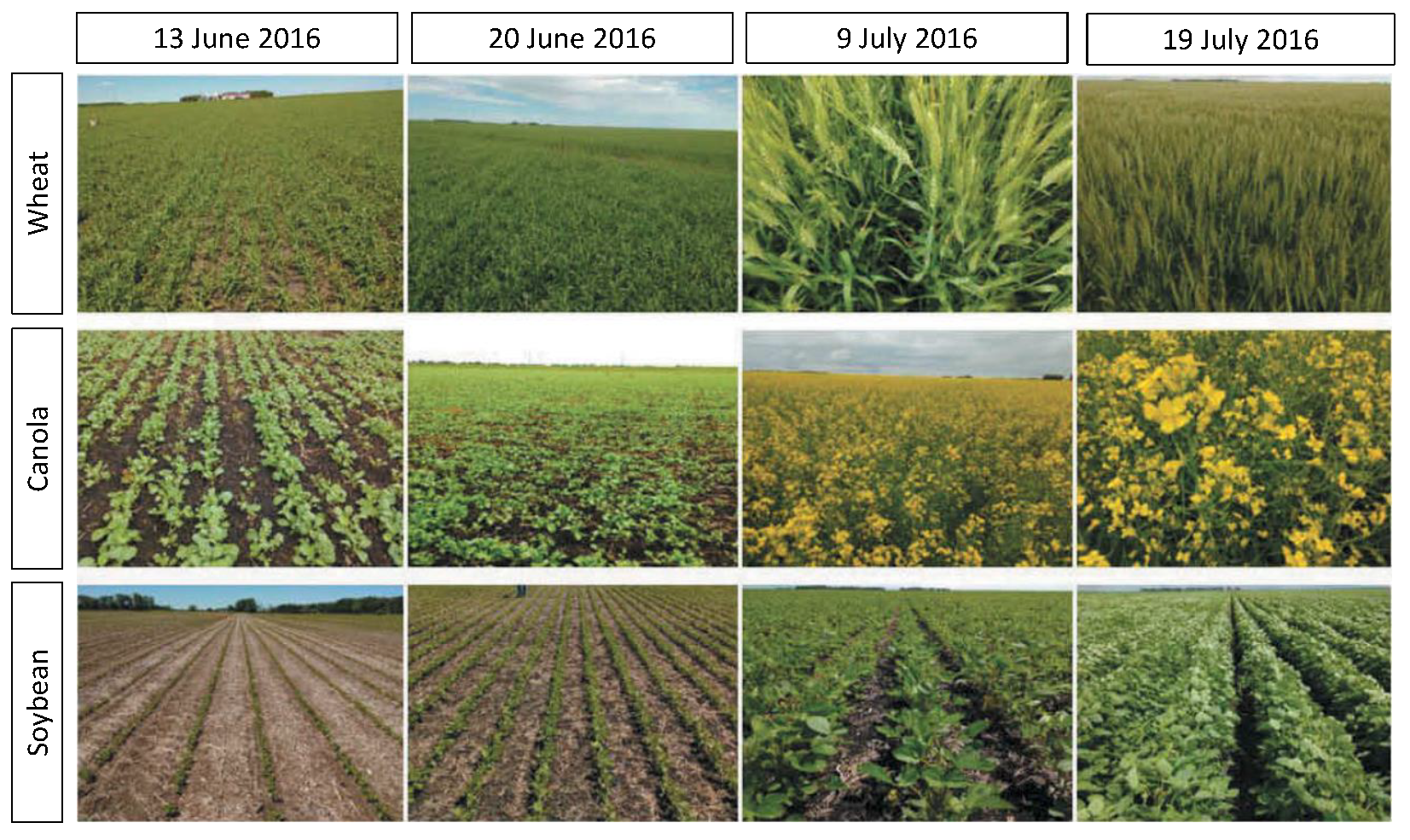
2. Study Area and Dataset

The study area is located at 49°34′21.5″ N, 97°55′43.1″ W South-West of Winnipeg, Manitoba in Canada. An overview of the study area can be seen in Figure 1. The test area has an extent of $26 \mathrm{k}\mathrm{m}\times 48 \mathrm{k}\mathrm{m}$. Several RADARSAT-2 images were acquired over this test area during the Soil Moisture Active Passive Validation Experiment 2016 Manitoba (SMAPVEX16-MB) [46,47]. The RADARSAT-2 acquisitions covered most of the fields sampled during the SMAPVEX16-MB campaign [48].

The site has a sharp divide in soil textures. Clay and fine loam soils account for ≈76% of this study domain, while coarse loam and sand soils account for ≈14%. Major annual crops grown in this area are spring wheat, soybeans, canola, and corn, which account for more than 90% of the area. Field data were collected during two Intensive Observation Periods (IOPs). The first IOP was conducted from June 08–20 during early vegetative growth. The second IOP was held during July 10–22, leading up to maximum biomass accumulation. The field photographs indicating various vegetative growth stages of the annual crops are shown in Figure 2.

2.1. Sampling Strategy

During the field campaign, a total number of 50 fields of various crops were selected for sampling. The nominal field size in this study area was $800 \mathrm{m}\times 800 \mathrm{m}$. In each field, soil moisture and vegetation sampling was conducted as shown in Figure 1. Soil moisture was measured at 16 sampling points arranged in two parallel transects, with each transect containing eight sampling points. Sampling points were separated by approximately 75 $\mathrm{m}$, and each transect was separated by 200 $\mathrm{m}$. Vegetation sampling was performed at three locations (i.e., points 2, 11, 14 in the first week and 3, 10, 13 in the second week of each IOPs) out of 16 sampling locations. Plant Area Index (PAI), biomass, and plant height were measured at these six sampling locations.

2.2. SAR Data Processing

RADARSAT-2 full polarimetric (HH, HV, VV) data were acquired in Fine Quad Wide Swath (FQ7W) mode and with incidence angles ranging from 24.98° to 28.32°. Four single-look complex (SLC) scenes acquired on 15 June 2016, 23 June 2016, 9 July 2016, and 17 July 2016 were preprocessed to generate the $3\times 3$ polarimetric covariance matrix $\mathbf{C}$. Subsequently, 1 (range) × 2 (azimuth) multi-looking was applied to obtain a square pixel of 10 $\mathrm{m}$. The refined Lee filter with a window size of $5\times 5$ was used to reduce speckle. The details of the RADARSAT-2 data and in situ data are given in

Table 1. Specifications of RADARSAT-2 data acquisitions and in situ measurements used in the present study.

Acquisition Date	Day of Year (DOY)	Beam Mode	Incidence Angle Range (Deg.)	In-Situ Measurement Window
15 June 2016	167	FQ7W	24.98–28.32	13 June, 15 June
23 June 2016	175	FQ7W	24.98–28.32	18 June, 20 June, 27 Jun
9 July 2016	191	FQ7W	24.98–28.32	6 July, 11 July, 12 July
17 July 2016	199	FQ7W	24.98–28.32	17 July, 20 July, 21 July

.

3. Methodology

3.1. Gaussian Process Regression

Gaussian Process Regression (GPR) belongs to the class of kernel-based methods in machine learning due to its flexibility to utilize diverse kernels depending on the types of data under analysis. In remote sensing applications, different kernel-based methods like Support Vector Machine (SVM), Relevance Vector Machine (RVM) [49] and GPR have been investigated for biophysical parameters retrieval in the literature. Among them, GPR [42] has shown promising results in comparison to other non-linear non-parametric methods. In the present study, we discuss the comparison between SVR and GPR methods. Gaussian Processes (GPs) are non-parametric probabilistic approaches used for regression and classification problems. Like a Gaussian distribution, a Gaussian Process is defined by its mean function and covariance (kernel) function. The kernel quantifies the similarity among the features utilized by GPR to predict the biophysical parameters. A Bayesian framework is used to train the GPs.

3.1.1. Notations

Gaussian Processes (GPs) can be explained in different ways, one of which is the function space approach. As defined in [50] a Gaussian Process can be defined as a collection of random variables, a finite number of which follows a joint normal distribution. The GPs follow a Bayesian framework and assume a prior distribution over the possible set of functions. The available data are then used to update its belief about the most suitable function that fits the data. The prior and the likelihood are assumed to follow a Gaussian distribution. As such, the aim is to learn a function f which will be able to predict the unknown biophysical parameters (target variables) $\mathit{y}$ from a set of input features, $\mathit{x}$ which in our case are the linear polarizations. An additive noise model $\mathit{y}=f\left(x\right)+\epsilon$, has been assumed, where the noise follows a standard normal distribution with 0 mean and variance ${\sigma }_n$, $\epsilon \backsim \mathcal{N}(0,{\sigma }_n^2)$. Thus the joint distribution of the training target values y and the unknown functions denoted with an asterisk ${\mathit{f}}_{*}$ is given by,

$$\left(\begin{array}{c}\mathit{y}\\ {\mathit{f}}_{*}\end{array}\right)\backsim \mathcal{N}\left(\begin{array}{c}0,\left(\begin{array}{cc}\mathit{K}+{\sigma }_n^2\mathit{I}& {\mathit{K}}_{*}\\ {\mathit{K}}_{*}^T& {\mathit{K}}_{**}\end{array}\right)\end{array}\right)$$

(1)

where the terms $\mathit{K}$ signifies the co-variance matrix between the observed feature values $x_i$ and $x_j$ with elements $k(x_i,x_j)$, ${\mathit{K}}_{*}$ denotes the co-variance matrix between the observed feature values and the test feature values with elements $k(x_i,x_{*})$ and finally the ${\mathit{K}}_{**}$ represents the matrix containing the variances between the test features with elements $k(x_{*},x_{*})$. If the dataset has N training points then the matrix $\mathit{K}$ is a $N\times N$ matrix. Similarly if there are $N_{*}$ test data points then the ${\mathit{K}}_{*}$ is a $N\times N_{*}$ matrix. The role of the co-variance matrix is explained in the next section.

3.1.2. Kernel Functions

A similarity measure is a very crucial aspect when it comes to learning-related algorithms. Therefore, covariance functions or kernels functions play a vital role in Gaussian Processes. Test points closer to the observed points perform better during the prediction phase. The $N\times N$ Gram matrix is said to be a covariance matrix if its elements are given by $k(x_i,x_j)$ where k is a covariance function. The gram matrix needs to be a positive semi-definite matrix to be considered a covariance matrix. Co-variance functions can be categorized into stationary, dot-product, non-stationary covariance functions. The role of these covariance or kernel functions is to capture the underlying linear and non-linear relationships among the features. During this study, we applied both linear and non-linear kernels have individually to understand their performances on the features. We utilized combinations to check their inherent characteristics. A homogeneous linear or dot-product kernel is represented by,

$$k(x_i,x_j)=x_i · x_j^T$$

(2)

and a squared exponential kernel is represented by,

$$k(x_i,x_j)={\sigma }_f^{2}exp\left(\frac{-{∥x_i-x_j∥}^2}{2l^2}\right)$$

(3)

The Radial Basis Function (RBF) kernel has two hyper-parameters ${\sigma }_f$ known as RBF variance and l known as the length scale of RBF, which are optimized during the training phase as discussed in Section 3.1.4. Our analysis demonstrated that the combination of linear and RBF kernels resulted in a relatively better retrieval accuracy than a homogeneous linear or non-linear RBF kernel. From the result, it was evident that the linear combination of those two kernels adequately captured the underlying linear and non-linear pattern of the data. Hence, in this study, we use a combination of a linear or dot product kernel, a non-linear RBF kernel, and a zero-mean Gaussian additive noise to retrieve the biophysical parameters;

$$k(x_i,x_j)=x_i · x_j^T+{\sigma }_f^{2}exp\left(\frac{-{∥x_i-x_j∥}^2}{2l^2}\right)+{\sigma }_n^2{\delta }_{ij}$$

(4)

where ${\delta }_{ij}$ represents a Kronecker delta function.

3.1.3. Prediction

The posterior predictive distribution over the most suitable functions for the dataset is obtained by conditioning out the known data and the unseen observations from the posterior distribution. Thus the predictive distribution of the Gaussian Process is given by,

$${\mathit{f}}_{*}\mid \mathit{X},\mathit{y},{\mathit{X}}_{*}\backsim \mathcal{N}(\widehat{{\mathit{f}}_{*}},{\Sigma }_{*})$$

(5)

where the mean of this predictive distribution $\widehat{{\mathit{f}}_{*}}$ gives the point estimate of the target variable which we are trying to retrieve, and the covariance ${\Sigma }_{*}$ indicates the uncertainty estimate of the retrieved biophysical parameter. The advantage of obtaining the uncertainty estimate makes GPs preferable as a prediction model because it indicates the model’s performance in predicting unknown data. The following expressions give the mean and variance of the predictive distribution,

$$\widehat{{\mathit{f}}_{*}}={\mathit{K}}_{*}^T{[\mathit{K}+{\sigma }_n^2 \mathit{I}]}^{-1}\mathit{y}$$

(6)

$${\Sigma }_{*}={\mathit{K}}_{**}-{\mathit{K}}_{*}^T{(\mathit{K}+{\sigma }_n^2 \mathit{I})}^{-1}{\mathit{K}}_{*}$$

(7)

The mean of the predictive distribution is a linear combination of the observed targets and not inputs and thus GPs are often called as $linear$ $smoother$ not $linear$ $predictor$.

3.1.4. Optimization

An important aspect of Gaussian Process regression models is their kernel hyper-parameters. These parameters assist in providing proper shape and fitting the functions to the data in the functions space. Correct estimation and tuning of these hyper-parameters are vital in preparing the powerful Gaussian Process models to be exploited to their full extent. Choosing a proper co-variance function and optimizing these hyper-parameters falls under the category of model selection problem. Co-variance functions like a squared exponential kernel function as mentioned in Equation (3), can be represented using two hyper-parameters l and ${\sigma }_f$, where l is the length scale of the kernel function and ${\sigma }_f$ is the RBF kernel variance. In an additive noise model, we assume a Gaussian distributed noise. The kernel hyper-parameters (l, ${\sigma }_f$) along with noise variance given by ${\sigma }_n$ must also be optimized for a particular noisy dataset. A common approach in Gaussian Process model selection problems for optimizing hyper-parameters is to maximize the log of marginal likelihood or the evidence of the process. The log marginal likelihood is expressed as,

$$logp(\mathit{y}\mid \mathit{\theta },{\sigma }_n)=log\mathcal{N}(\mathit{y}\mid 0,\mathit{K}+{\sigma }_n^2 \mathit{I})$$

(8)

In the above expression, $\mathit{\theta }$ represents the set of all the model hyper-parameters that require optimization. The log marginal likelihood is not generally convex in a Gaussian Process; thus, multiple initializations may be necessary, which becomes time-consuming and may lead to local minima. Therefore a gradient-based approach is used to save time and to improve efficiency.

3.2. Data Preparation

This study used in situ measurements from various wheat, canola, and soybean fields to train and validate the model. The datasets consist of the field measurements collected during the Intensive Observation Periods (IOPs) in June and July. Specifically, measurements collected close in time to the SAR acquisitions (15 June, 23 June, 9 July, and 17 July) were used. The data from all four dates were randomly split into training (70%) and validation (30%) data sets. The training and the test dataset consists of the linear polarizations (HH, HV, VV) as the features and PAI, WB, VWC as the target variables.

3.2.1. Data Skewness Analysis

The backscatter coefficients obtained from the processed RADARSAT-2 images and the in situ measurements of the biophysical parameters do not follow a standard normal distribution. This may result from the random distribution of crops over the study area and the non-normal growth curve over the season. The skewness of the data affects the performance of statistical models, particularly those models that assume that the data follow a normal distribution. In skewed data, the points in the tail region act as outliers and degrade the model’s performance. In these cases, it is necessary to transform the raw data to bring the underlying distribution close to a Gaussian or normal distribution. Various techniques are utilized for data transformation in machine learning and to deal with non-normal distributed data sets.

In our study, the features (HH, HV, VV) and the target variables (PAI, WB, VWC) for all three crops types are skewed. Skewness in the data has been reduced by applying a Box-Cox transformation [51]. The skewness values of each of the linear polarizations before and after the transformation are presented in

Table 2. Initial and final skewness of linear polarizations and PAI before and after Box-Cox transformation.

Crop	Variables	Initial Skewness	$\mathit{\lambda }$ Values	Final Skewness
Wheat	HH	1.293	−0.013	$2.8\times {10}^{-5}$
	HV	2.437	−0.569	$5.6\times {10}^{-2}$
	VV	1.222	−0.379	$3.7\times {10}^{-2}$
	PAI	−0.270	1.120	−$1.9\times {10}^{-1}$
Canola	HH	0.898	−0.122	$1.2\times {10}^{-2}$
	HV	1.995	0.200	$5.9\times {10}^{-2}$
	VV	0.515	0.220	−3.$7\times {10}^{-2}$
	PAI	0.246	0.519	−$1.9\times {10}^{-1}$
Soybean	HH	1.090	−0.310	$3.2\times {10}^{-2}$
	HV	1.550	−0.311	$5.7\times {10}^{-5}$
	VV	0.698	0.009	−$2.0\times {10}^{-3}$
	PAI	0.819	0.149	−$8.5\times {10}^{-2}$

for PAI for wheat, canola, and soybean crops and

Table 3. Initial and final skewness of linear polarizations, WB and VWC before and after Box-Cox transformation.

Crop	Variables	Initial Skewness	$\mathit{\lambda }$ Values	Final Skewness
Wheat	HH	1.108	0.027	−$4.1\times {10}^{-4}$
	HV	1.789	−0.365	$2.1\times {10}^{-2}$
	VV	1.192	−0.494	$6.2\times {10}^{-2}$
	WB	0.150	0.754	−$1.2\times {10}^{-1}$
	VWC	0.311	0.693	−$7.5\times {10}^{-2}$
Canola	HH	0.675	0.179	−$1.9\times {10}^{-2}$
	HV	1.325	0.305	$3.6\times {10}^{-2}$
	VV	0.869	0.252	−$2.7\times {10}^{-2}$
	WB	0.089	0.644	−$2.1\times {10}^{-1}$
	VWC	0.069	0.673	−$2.1\times {10}^{-1}$
Soybean	HH	0.859	−0.034	$4.0\times {10}^{-3}$
	HV	1.548	−0.398	$7.8\times {10}^{-2}$
	VV	0.909	0.004	−$5.2\times {10}^{-4}$
	WB	1.552	0.042	−$1.4\times {10}^{-2}$
	VWC	1.567	0.043	−$1.5\times {10}^{-2}$

for WB and VWC. After the transformation, skewness is reduced for features and the target variables, making them suitable as predictors and target variables for evaluating the machine learning model. The $\lambda$ value mentioned in Table 2 and Table 3 indicates the power to which each data is raised. The Box-Cox transformation is first applied on the training data to obtain the optimum value of $\lambda$ between $-5$ and 5. The optimum $\lambda$ values are then utilized to transform the test dataset.

3.2.2. Experimental Design

The Gaussian Process Regression model has been developed with the RADARSAT-2 measured backscatter intensities and the in situ measured crop parameters as the response. GPR has been modeled using the GPy library [52]. It is a Gaussian Process framework written in Python, developed by the Sheffield machine learning group. Subsequently, an experimental setup is designed to build the GPR models with different predictor combinations. The experiment has been designed with different co-pol and cross-pol combinations of backscatter intensities. The different predictor combinations considered for the experiment are HH+HV, HV+VV, HH+VV, and HH+HV+VV. However, the target variables (crop parameters) remain the same for each experiment and for all the crops during the training phase. The trained GPR models are utilized during the prediction phase to estimate the biophysical parameters for the validation dataset. The GPR model hyper-parameters which are tuned to achieve high precision and accuracy are: l, ${\sigma }_f$ and ${\sigma }_n$. The hyper-parameters have been discussed in Section 3.1.2. A scaled conjugate gradient-based approach with 1000 iterations is used to obtain the optimized values of these hyper-parameters.

This research also conducted a comparative analysis between GPR, SVR, and RFR. SVR and RFR were implemented using the open-source Python Scikit-learn packages. SVR is a generalized version of a Support Vector Machine (SVM) [53] designed for regression-based problems [54]. Similar to GPR, it is also a kernel-based method utilized in the literature to estimate biophysical parameters. In the case of SVR, the model hyper-parameters which are tuned during optimization are Kernel (the type of kernel to be used by the algorithm), Gamma (controls the influence of the decision boundary), and C (regularization parameter). The optimized values of these hyper-parameters have been obtained using a cross-validated Random Search. A k-fold cross validation technique was implemented with k being the number of folds was specified as 10. The cross-validation technique is a powerful approach towards preventing overfitting.

Random Forest Regression (RFR) is a tree-based ensemble technique that uses bagging or bootstrap aggregation to average the predictions from multiple decision tree models [55]. This approach helps in reducing variance and chances of high error. The hyper-parameters of the RFR model include: n_estimators (number of decision trees), max_depth (maximum depth of each decision tree), min_samples_split (minimum number of samples required to split an internal leaf node) and min_samples_leaf (minimum number of samples required to be at a leaf node). These hyper-parameters were obtained from a k-fold cross-validated random search on a range of possible values. Besides random search the two very sensitive hyper-parameters n_estimators and max_depth were analyzed utilizing Out Of Bag score (OOB score).

The efficiency of the models is assessed using Pearson-correlation coefficient ($\rho$) and error estimates including Root Mean Square Error (RMSE) and Mean Absolute Error (MAE) for every experimental setup and for each individual crop.

4. Results and Discussions

This section describes the important considerations for an operational crop monitoring application. The sensitivity of the backscatter coefficients to the condition of the crops on each acquisition date is first assessed. Next, the correlation among the backscatter coefficients and the vegetation biophysical parameters (PAI, WB, and VWC) is examined to understand variations in scattering due to changes in crop growth stages and canopy structures and the impact of incidence angle over the entire observation period. A GPR model was used to estimate the biophysical parameters of wheat, canola, and soybeans. Following the steps described in Section 3.1 and Section 3.2. A comparative analysis between GPR, SVR, and RFR is also presented based on retrieval accuracies for all the crops.

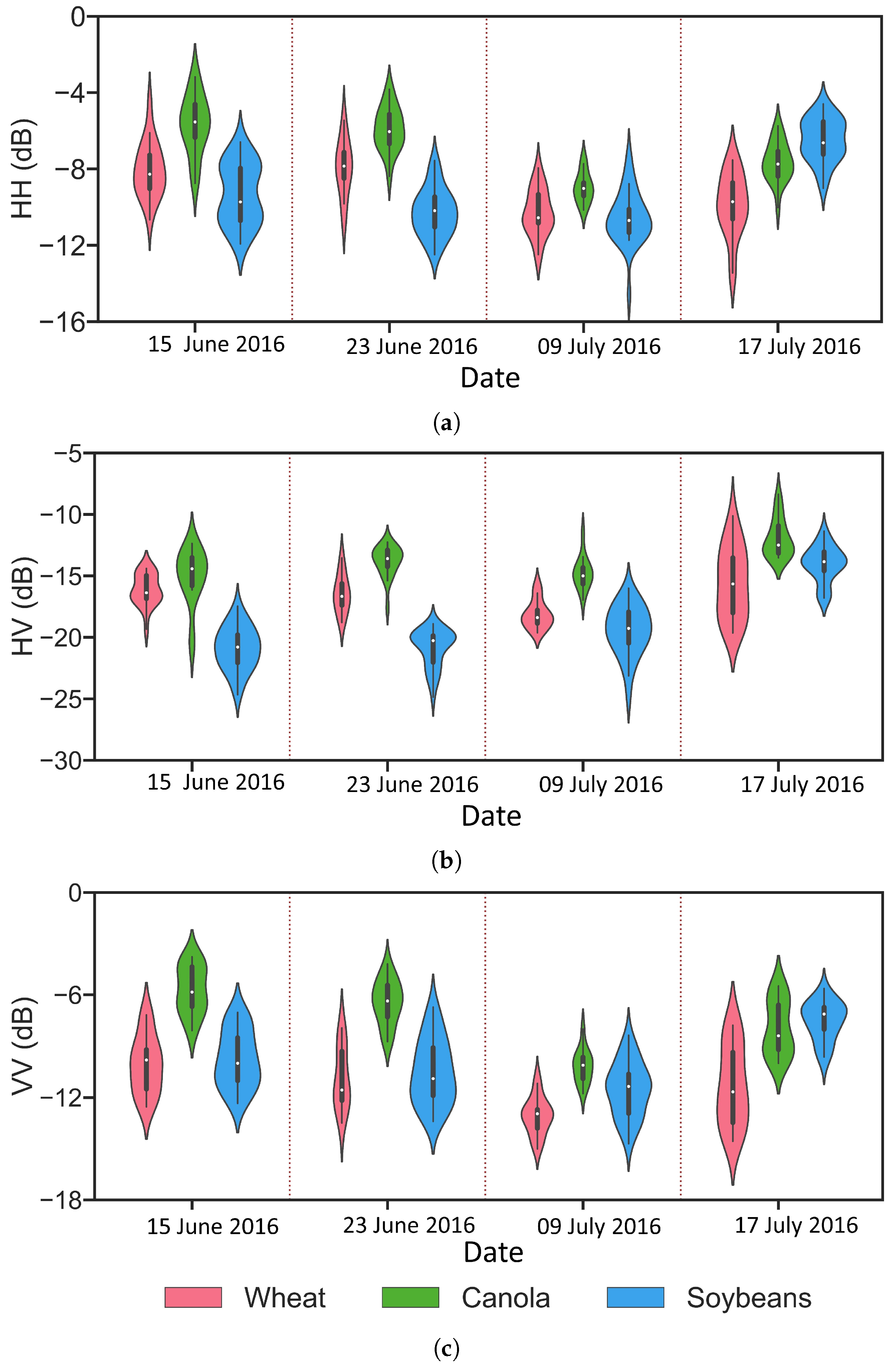
4.1. Sensitivity Analysis of HH, HV, VV to Crop Development

The temporal variation of the backscatter coefficients on a linear basis (i.e., HH, HV, VV) are plotted in Figure 3 as violin plots for the three crop types. The plots illustrate the distribution of the sample points across all observation periods. Each violin plot comprises a Kernel Density Estimate (KDE) plot and a box plot. Within the KDE plot lies the box plot that represents the median (white dot) and the inter-quartile range (darker line) for the particular backscatter coefficient. A violin plot captures the distribution of the sample points across different backscatter coefficient values and identifies the presence of outliers and a multi-modality if present in the data.

4.1.1. Wheat

Temporal variability of HH, HV, VV backscatter intensities for wheat is shown in Figure 3a–c, respectively. On the 15 June, wheat is in its early tillering stage. The median HH backscatter value on 15 June is $-8.27$ dB. This high return in the HH backscatter is due to low vegetation cover at this early development stage. Consequently, the backscatter return is largely influenced by the soil surface. Between the 15 and 23 of June, HH backscatter for wheat shows an increasing trend. On 23 June, the median value of HH backscatter is $-7.85$ dB. At this phenological period, wheat advances from its tillering stage towards booting through stem elongation stages. As the density of the crop increases, the radar wave interacts more with the horizontal portion of the leaf, causing more HH backscatter return. In the first week of July, wheat reaches its early flowering, and HH backscatter declines to $-10.55$ dB during this period as the canopy volume increases. This reduction may be due to attenuation in the upper crop canopy by the wheat heads. On 17 July, when wheat reaches its early dough stage, backscatter increases to $-9.71$ dB. As the crop advances towards maturity and ripening, wheat kernels begin to dry, and overall canopy water content declines. During this period, the KDE plot has a longer tail towards lower values of HH (<$-12$ dB). The rate of senescence or dry down will be impacted by many factors, including the timing of seeding and soil properties. This longer tail during this phenological period suggests variations in senescence among these wheat fields.

At the time of tillering, the wheat canopy cover is still sparse, and with a limited volume to create random scattering, the HV response is low ($-16.67$ dB). A bi-modal distribution of HV backscatter for wheat can be seen during 15 June, most likely due to two different sources of scattering. Some wheat canopies have started to boot, while others remain at the tillering stage. After June, the crop progresses towards its dough stage and maturity around 17 July. HV backscatter for wheat increases to $-15.65$ dB. With increased canopy volume, multiple scattering from the wheat heads causes HV backscatter to increase. The KDE plot for 17 July shows a flat distribution indicating an equal distribution of HV backscatter responses around the median.

On 15 June, the median of VV backscatter is higher around $-9.80$ dB. As the phenology progresses from booting towards flowering, VV backscatter declines from $-11.56$ dB on 23 June reduces to $-12.95$ dB on 9 July. During this period, the volume fraction of the vegetation starts to increase. This increase in canopy volume results from the accumulation of leaves and lengthening of the stems. With an increase in attenuation from the predominantly vertical structure of the wheat stems, the VV backscatter is reduced [56,57]. On 17 July, there is an observed increase in VV backscatter to $-11.67$ dB a result of the increase in biomass during the dough stage.

4.1.2. Canola

Canola is at its leaf development stage during the early phenological period (15 June). HH backscatter during this period is high ($-5.53$ dB), likely due to a dominance of scattering from the soil given the low canopy cover at this early stage of canola development. After 15 June, the crop progresses from its leaf development stage towards inflorescence emergence. As the crop height increases and the canopy cover progresses, the soil contribution to the SAR backscatter is reduced. HH backscatter during this period declines from −5.53 dB to −6.04 dB. Around 9 July, as the canopy volume increases, the incident radar wave is depolarized by the complex canopy structure of the canola. This further reduces HH backscatter to $-9.02$ dB on 9 July. Canola reaches its early pod development stage on 17 July, and HH backscatter increases by $1.28$ dB.

The median HV backscatter response is $-14.42$ dB on 15 June. The canopy is less developed during its leaf development stage, more soil is exposed, and greater scatter originates from the soil. This variation in scattering is evident in the long left tail of the KDE plot of HV backscatter. As the crop progresses towards inflorescence emergence around 23 June, cross-polarization backscatter increases from −14.42 dB to −13.59 dB during this period. The formation of pods in the canola crop creates a complex geometric structure and increases in the volume of the canopy. During this phenology stage, around 17 July HV backscatter increases to $-12.49$ dB.

During the leaf development stage of canola around 15 June, VV backscatter was approximately $-5.84$ dB. As the crop develops, buds and flowers emerge VV backscatter declines sharply. As seen in Figure 3c, VV backscatter reaches a minimum of $-10.10$ dB during the flowering stage around 9 July. The buds and the flowers, which have a small structure, prevent the scattering of the underlying canopy, thus decreasing VV backscatter [15,58]. On 17 July, the stem of the canopy plant had a greater volume than the flowers. VV backscatter response increases from −10.10 dB to −8.40 dB as the vertical structure of the canopy begins to dominate.

4.1.3. Soybean

Soybeans and canola have comparable sensitivities to HH backscatter. On 15 June, soybeans are beginning to develop leaves, and backscatter in the HH polarization is $-9.72$ dB. Between 15 June and 23 June, leaf development progresses towards the fifth trifoliate stage [59] and HH backscatter declines to $-10.18$ dB. As the side shoots begin to form, scattering from the soybean canopy increases. On 19 July, soybeans reached the flowering stage. HH backscatter increases by $4.07$ dB during this period, as evident from Figure 3a. During 15 June and 17 July, HH has a bi-modal distribution, and on 9 July, backscatter has a distribution with a comparatively longer tail indicating outliers towards lower HH (<$-14$ dB) values. These outliers may be due to the variations in growth stages among fields depending on the time of seeding and uneven growth due to different soil properties. Earlier seeded fields would present larger canopies and greater canopy volume scattering.

During the leaf development stage of soybean, HV backscatter is lower with a median backscatter of $-20.78$ dB on 15 June. A sparse canopy attenuates little of the incident waves and allows for greater scattering from the soil. The crop progresses towards pod development and flowering stage from 23 June to 17 July. With a more complex canopy structure, random scattering events within the canopy increase. On 9 July, the HV backscatter for soybeans is $-20.26$ dB. Cross polarization backscatter on 17 July for the soybean canopies increases to $-13.84$ dB due to an accumulation of biomass and reduction in scattering from the soil [15].

VV backscatter during the leaf development stage of soybean is high. The median VV backscatter response is around $-9.99$ dB. As pods develop on the soybean plants, VV backscatter falls by $-1.36$ dB, reaching a minimum on 9 July as evident from Figure 3c. A dense canopy structure prevents any backscatter return from the soil until the crop begins to form flowers and pods (around 17 July) that VV backscatter increases by $4.22$ dB.

4.2. Correlation Analysis: Backscatter vs. Biophysical Parameters

Correlation analysis assists in deciphering the impacts of changing biophysical and phenological states on SAR backscatter. First, we analyzed the correlation for each crop for each date individually. Correlation between the backscatter coefficients and the biophysical parameters for 15 June, 23 June, 9 July, and 17 July are symbolized as ${\rho }_{{\sigma }^o}^{15}$, ${\rho }_{{\sigma }^o}^{23}$, ${\rho }_{{\sigma }^o}^9$ and ${\rho }_{{\sigma }^o}^{17}$, respectively. In addition, the overall correlation (${\rho }_{{\sigma }^o}^o$) between the linear polarization and the biophysical parameters was computed by considering all the sample points from all the dates altogether.

4.2.1. Wheat

Correlation among the backscatter coefficients and biophysical parameters for wheat are listed in

Table 4. Pearson correlation ($\rho$) between biophysical parameters and linear-polarizations (HH, HV, VV) for wheat. Statistically significant correlations at 95% confidence level are shown in bold.

	${\mathit{\sigma }}^{\mathit{o}}$	${\mathit{\rho }}_{{\mathit{\sigma }}^{\mathit{o}}}^{15}$	${\mathit{\rho }}_{{\mathit{\sigma }}^{\mathit{o}}}^{23}$	${\mathit{\rho }}_{{\mathit{\sigma }}^{\mathit{o}}}^9$	${\mathit{\rho }}_{{\mathit{\sigma }}^{\mathit{o}}}^{17}$	${\mathit{\rho }}_{{\mathit{\sigma }}^{\mathit{o}}}^{\mathit{o}}$
PAI	HH	−0.63	−0.35	−0.18	0.26	−0.57
	HV	−0.12	−0.73	−0.39	0.49	0.05
	VV	−0.59	−0.68	−0.29	0.12	−0.69
WB	HH	−0.08	−0.69	−0.26	−0.16	−0.51
	HV	−0.01	−0.19	−0.26	0.06	−0.23
	VV	−0.03	−0.65	−0.31	0.06	−0.47
VWC	HH	−0.09	−0.67	−0.20	−0.07	−0.47
	HV	−0.01	−0.18	−0.29	0.13	−0.24
	VV	−0.03	−0.63	−0.29	0.13	−0.46

. The significant correlations at 95% confidence level are highlighted in bold. When correlations are run on each date separately, the results are inconsistent among all biophysical parameters. Correlations are growth-specific, and it is only when the analysis is run using all dates of data that significant correlations are reported for all polarizations and biophysical parameters. The one exception is HV backscatter and PAI. Correlations are negative, indicating a decrease in scattering at higher biomass accumulations, suggesting greater attenuation. HH has a significant but negative correlation with PAI as the wheat advances from early tillering to booting stage. Correlation between HH backscatter and PAI for wheat on 15 June (${\rho }_{HH}^{15}$) is $-0.63$. when PAI varies from 0.83 m² m⁻² to 5.2 m² m⁻² (

Table A1. Temporal variations of Plant Area Index (PAI) (m² m⁻²), Wet-Biomass (WB) (kg m⁻²) and Vegetation Water Content (VWC) (kg m⁻²) for wheat, canola and soybean at different dates.

		15 June	23 June	9 July	17 July
Wheat	Phenology	Tillering stage	Booting stage	Early flowering stage	Early dough stage
	PAI	0.83–5.20	2.95–7.70	4.37–7.72	5.13–8.80
	WB	0.43–3.45	0.78–3.59	2.02–5.90	1.51–4.26
	VWC	0.36–2.99	0.67–3.01	0.97–4.86	0.97–3.05
Canola	Phenology	Leaf development	Inflorescence emergence	Flowering stage	Pod development
	PAI	0.39–1.79	0.16–6.12	1.82–6.35	3.64–8.33
	WB	0.21–1.99	0.78–3.79	1.80–5.03	2.60–4.47
	VWC	0.20–1.84	0.71–3.51	1.55–4.35	2.24–3.90
Soybean	Phenology	Leaf development	Fifth trifoliate stage	Pod development	Flowering stage
	PAI	0.07–0.94	0.01–0.55	0.27–5.70	0.25–4.18
	WB	0.02–0.13	0.03–0.42	0.07–1.45	0.13–1.63
	VWC	0.01–0.11	0.03–0.36	0.06–1.26	0.11–1.33

). After 15 June, as the canopy volume increases correlation between HV and PAI increases. On 23 June PAI varied between 2.95 m² m⁻² to 7.7 m² m⁻² and correlation with HV backscatter increases to $-0.73$. Wheat reached its dough stage on 17 July. HV shows a positive correlation with PAI during this phenological period of wheat. At the dough stage (17 July), only HV is correlated with PAI ($0.49$). VV backscatter has a higher correlation with PAI in the initial phenological stages of wheat. During early tillering VV backscatter had a correlation (${\rho }_{VV}^{15}$) of $-0.59$ increasing at booting stage (${\rho }_{VV}^{23}$) to $-0.68$. When all the sample points are considered from all observation dates, HH and VV had correlations with PAI of $-0.57$ and $-0.69$.

Correlations between HH backscatter and WB and VWC increase from tillering (15 June) to booting stages (23 June). WB for wheat on 15 June varied between 0.43 kg m⁻² and 3.45 kg m⁻² and VWC varied between 0.36 kg m⁻² and 2.99 kg m⁻² as documented in Table A1. During booting (23 June) biomass and water content further increased with WB between 0.78 kg m⁻² and 3.59 kg m⁻² and VWC between 0.67 kg m⁻² and 3.01 kg m⁻². Correlations with HH backscatter are negative ($-0.69$) for WB and $-0.67$ for VWC. On 9 July, the wheat is flowering and HV backscatter is correlated with WB ($-0.26$) and VWC ($-0.29$). The correlation of VV scattering and WB is slightly higher ($-0.31$). At flowering, correlations are for the most part, not statistically significant. When sample points from all the observation dates are pooled, HH and VV backscatter have a higher correlation with WB and VWC when compared with HV backscatter.

4.2.2. Canola

As evident from

Table 5. Pearson correlation ($\rho$) between biophysical parameters and linear-polarizations (HH, HV, VV) for canola. Statistically significant correlations at 95% confidence level are shown in bold.

	${\mathit{\sigma }}^{\mathit{o}}$	${\mathit{\rho }}_{{\mathit{\sigma }}^{\mathit{o}}}^{15}$	${\mathit{\rho }}_{{\mathit{\sigma }}^{\mathit{o}}}^{23}$	${\mathit{\rho }}_{{\mathit{\sigma }}^{\mathit{o}}}^9$	${\mathit{\rho }}_{{\mathit{\sigma }}^{\mathit{o}}}^{17}$	${\mathit{\rho }}_{{\mathit{\sigma }}^{\mathit{o}}}^{\mathit{o}}$
PAI	HH	0.55	−0.30	−0.21	0.09	−0.51
	HV	0.27	0.38	0.31	−0.01	0.47
	VV	0.28	−0.12	0.01	0.02	−0.48
WB	HH	0.26	0.56	−0.06	−0.43	−0.55
	HV	0.43	0.51	−0.20	−0.64	0.13
	VV	−0.04	0.41	−0.55	−0.10	−0.58
VWC	HH	0.26	0.56	−0.10	−0.48	−0.54
	HV	0.41	0.52	−0.24	−0.66	0.12
	VV	−0.03	0.40	−0.57	−0.14	−0.57

backscatter and biophysical parameters are not significantly correlated when analyzed for individual dates. The only exception is HH backscatter and PAI on 15 June when PAI is between 0.39 m² m⁻² and 1.79 m² m⁻² when the leaves of canola are beginning to develop. At this early stage, the soil has little cover (Table A1). Despite the rapid growth of the canola canopy throughout the experiment (PAI from 0.16 m² m⁻² to 8.33 m² m⁻², WB from 0.21 kg m⁻² to 4.47 kg m⁻² and VWC from 0.20 kg m⁻² to 3.90 kg m⁻²) backscatter is not correlated with these parameters measured on individual dates. It is only when all data are pooled that correlations are significant. When sampling points from all the observation periods are considered, HH and VV backscatter showed a significantly higher correlation with PAI when compared with HV backscatter. In addition, HH and VV backscatter showed a significant correlation with biophysical parameters WB and VWC in contrast to HV backscatter.

4.2.3. Soybeans

Soybeans are a broadleaf crop and in this region of Canada are typically seeded by the third week of May and harvested in early September [60]. In June, soybeans are in an early vegetative stage with initial leaves developing, and as a result, the soil has a major contribution to overall scattering. On 15 June, most soybean fields are in the unifoliate to the third trifoliate stage. During this stage PAI varies between 0.07 m² m⁻² to 0.94 m² m⁻².

Backscatter coefficients did not show any significant correlation with PAI on 15 June. After 15 June, soybean crops advanced into the fifth trifoliate stage. HV backscatter shows a higher correlation with PAI during this phenological period. On 23 June, the correlation of HV backscatter with PAI increases to 0.55. The fifth trifoliate stage of soybean is followed by pod development at the beginning of July. PAI during this period varied between 0.27 m² m⁻² to 5.70 m² m⁻². It is evident from

Table 6. Pearson correlation ($\rho$) between biophysical parameters and linear-polarizations (HH, HV, VV) for soybean. Statistically significant correlations at 95% confidence level are shown in bold.

	${\mathit{\sigma }}^{\mathit{o}}$	${\mathit{\rho }}_{{\mathit{\sigma }}^{\mathit{o}}}^{15}$	${\mathit{\rho }}_{{\mathit{\sigma }}^{\mathit{o}}}^{23}$	${\mathit{\rho }}_{{\mathit{\sigma }}^{\mathit{o}}}^9$	${\mathit{\rho }}_{{\mathit{\sigma }}^{\mathit{o}}}^{17}$	${\mathit{\rho }}_{{\mathit{\sigma }}^{\mathit{o}}}^{\mathit{o}}$
PAI	HH	−0.09	0.09	0.26	0.03	0.39
	HV	0.23	0.55	0.56	0.32	0.64
	VV	−0.25	−0.08	0.47	0.26	0.31
WB	HH	0.34	0.11	−0.01	−0.09	0.38
	HV	−0.01	0.54	0.54	0.56	0.77
	VV	0.23	−0.06	0.09	0.26	0.34
VWC	HH	0.33	0.10	−0.01	−0.09	0.37
	HV	−0.01	0.56	0.54	0.56	0.76
	VV	0.21	−0.08	0.09	0.26	0.33

that the correlation between HV and VV backscatter and PAI increases during this period. When the overall correlation between backscatter coefficients and PAI were analyzed, HV backscatter had a higher correlation with PAI when compared with HH and VV backscatter.

WB varies between 0.02 kg m⁻² and 1.63 kg m⁻² covering the entire phenological period of soybean development. Among the backscatter coefficients, HV significantly correlates with WB as the crop progresses from its fifth trifoliate stage towards flowering. A similar trend can be seen while analyzing the correlation between HV backscatter and VWC. An overall correlation analysis between the backscatter coefficients and the biophysical parameters WB and VWC indicates that HV backscatter has the highest correlation. HH and VV backscatter showed similar sensitivity towards WB and VWC.

The correlation between the biophysical parameters of the crops and the backscatter coefficients vary depending upon the phenological stages of the crops. This occurs because the radar backscatter returns are highly influenced by the canopy structure, soil characteristics, crop growth stage, and radar incidence angle.

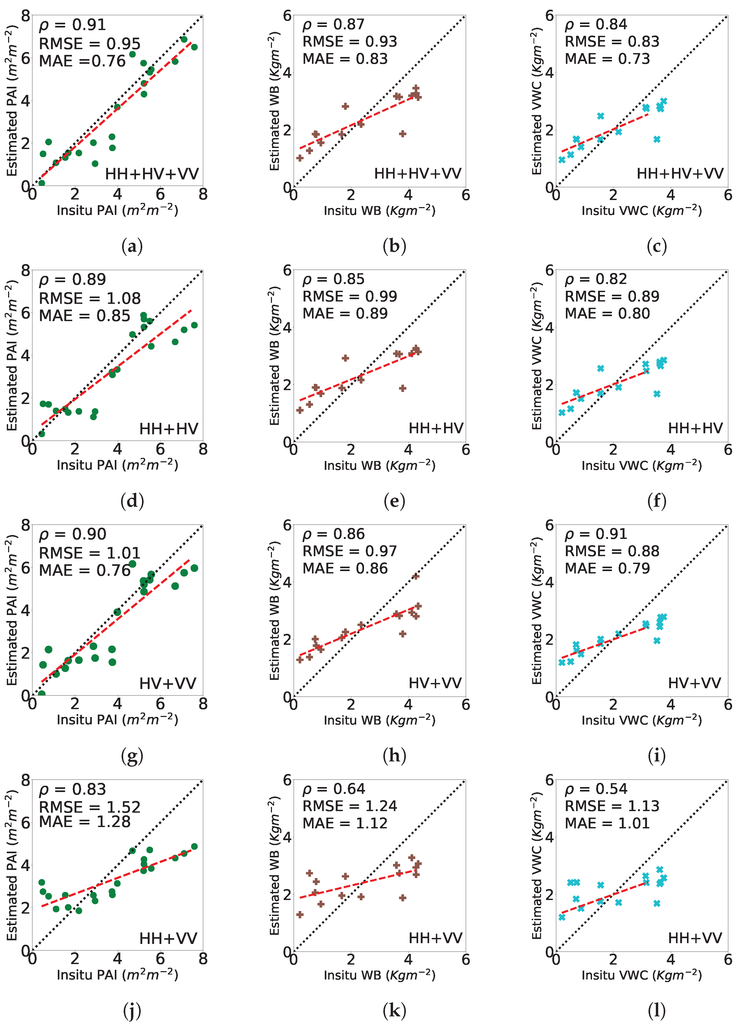
4.3. Biophysical Parameter Estimation

The GPR model inversion utilizes dual-pol (HH+HV, HV+VV, and HH+VV) and full-pol (HH+HV+VV) combinations of backscatter intensities as predictors to the model. The retrieval accuracy of the models for PAI, WB, and VWC are assessed for wheat, canola, and soybean using the validation dataset.

4.3.1. Wheat

The GPR inversion methodology evaluates the retrieval accuracy of PAI, WB, and VWC. The in situ measured PAI varied from 0.83 m² m⁻² to 8.80 m² m⁻², covering early tillering to dough stages. The performance of the GPR model varies for different polarization combinations, as shown in Figure 4. Among the dual-pol combinations, the HV+VV outperformed HH+HV and HH+VV combinations.

As presented in Figure 4g the correlation between in situ PAI and estimated PAI for the HV+VV combination is higher than the HH+HV and HH+VV combinations. The correlation for the HV+VV combination is 0.78. In comparison, the HH+HV dual-polarization combination results in a correlation coefficient of 0.75 and for HH+VV, a coefficient of 0.64. When HV+VV is used with the GPR model, the root mean square error for PAI decreases by 5.8%. When HH+VV are used, RMSE declines by 17%. In Figure 4 the red dotted line represents the best fit line between the in situ and estimated biophysical parameter.

An improvement in retrieval accuracy is achieved using all polarizations for PAI estimations. The model showed a 6.4% increase in correlation between in situ PAI and estimated PAI when all polarizations are used. With these three polarizations as predictors in the GPR model, RMSE decreases by 9.8%. When PAI exceeds 7 m² m⁻² and plants reach the early flowering and dough stages, plant area is underestimated. In contrast, an overestimation is observed for PAI values less than 4 m² m⁻² when the plant is in the early tillering stage. A comparatively better estimation is reported for PAI values between 4 m² m⁻² and 7 m² m⁻² as the plant progresses from the booting stage towards the flowering stage. In summary, the GPR model, which includes either a dual-pol combination of HV+VV or a full pol combination of HH+HV+VV, could produce accurate estimates of PAI over the entire phenological period.

In the case of WB, the ground measured values varied from 0.43 kg m⁻² to 5.9 kg m⁻² as shown in Table A1. WB retrieval with a dual-pol combination of HH+HV and HV+VV showed comparable results. A saturation in the estimation of WB is evident towards the end of the heading stage of the wheat crop. A reduction of 2.4% in RMSE and 9.5% in MAE is evident when all three polarizations are used as compared to an HV+VV dual-pol combination. A previous experiment also used a dual-polarization HH and HV combination to retrieve the biomass of wheat using data from RADARSAT-2 [28].

VWC impacts the intensity of scattering from vegetation, and this biophysical parameter is important in determining crop stress and water needs. Measures of VWC were determined through drying and weighing of crop biomass, with VWC ranging between 0.36 kg m⁻² to 4.86 kg m⁻². HV+VV had the highest correlation among the dual-pol combinations when comparing in situ measured and model estimated VWC. An increase of 2.8% to 4.1% in the correlation coefficient was achieved utilizing the dual-pol HV+VV combination when compared with other dual-pol combinations. When all three polarizations were used, the errors associated with the estimation of water content were reduced (RMSE (0.68 kg m⁻²) and MAE (0.56 kg m⁻²)).

A two-tailed t-test was implemented to check the significance of the correlation between the estimated biophysical parameters of wheat and their in situ measurements at a 95% confidence level. As evident from

Table 7. Statistical significance of correlation coefficient ($\rho$) between estimated and in situ biophysical parameters at 95% confidence level for each linear polarization combinations in case of wheat.

	Linear Polarization Combinations	$\mathit{\rho }$	p-Value
PAI	HH+HV+VV	0.83	$2.67\times {10}^{-7}$
	HH+HV	0.75	$3.95\times {10}^{-16}$
	HV+VV	0.78	$3.80\times {10}^{-6}$
	HH+VV	0.64	$5.19\times {10}^{-4}$
WB	HH+HV+VV	0.66	$3.93\times {10}^{-7}$
	HH+HV	0.65	$5.94\times {10}^{-7}$
	HV+VV	0.64	$9.99\times {10}^{-7}$
	HH+VV	0.67	$1.65\times {10}^{-7}$
VWC	HH+HV+VV	0.63	$1.46\times {10}^{-6}$
	HH+HV	0.57	$1.68\times {10}^{-5}$
	HV+VV	0.60	$4.76\times {10}^{-6}$
	HH+VV	0.63	$1.23\times {10}^{-6}$

the biophysical parameters estimated by the GPR model show a significant correlation for all the polarization combinations.

A comparative analysis between GPR, Support Vector Regression (SVR), and Random Forest Regression (RFR) is provided in

Table 8. Comparing performance of GPR, SVR and RFR for estimating biophysical variables of wheat utilizing a dual-pol (HV+VV) combination. Statistical measures of GPR are highlighted in bold for each biophysical parameter.

	Algorithm	RMSE	MAE	$\mathit{\rho }$	R2
PAI	GPR	1.12	0.93	0.78	0.61
	SVR	1.39	1.09	0.63	0.40
	RFR	1.48	1.19	0.61	0.36
WB	GPR	0.83	0.63	0.64	0.41
	SVR	0.92	0.76	0.54	0.30
	RFR	0.86	0.72	0.60	0.36
VWC	GPR	0.69	0.55	0.60	0.37
	SVR	0.74	0.60	0.49	0.25
	RFR	0.68	0.56	0.59	0.35

for all wheat biophysical parameters. It is evident from our previous results in Figure 4 that in addition to the full-pol combination, the dual-pol combination of HV+VV is able to retrieve these biophysical parameters. Considering that HV+VV yielded promising results in estimating all biophysical parameters, this dual-polarization combination is used to compare the performance of these three machine learning algorithms.

In the case of wheat biophysical parameter estimation, GPR performed better than SVR and RFR in terms of error estimates (RMSE, MAE), correlation coefficient ($\rho$), and coefficient of determination (R²). In estimating PAI, SVR had a comparatively better performance than RFR in terms of error estimates and correlation. The GPR model showed a 24.32% decrease in RMSE relative to the RFR model and a 19.42% decrease in RMSE with respect to the SVR model. The correlation between in situ PAI and model estimated PAI increased by 27.86% with the GPR relative to the RFR and 23.80% when compared to the SVR model. In contrast, the RFR had a comparative performance to GPR in estimating WB. A similar performance was observed while retrieving VWC.

GPR delivered better estimates of the biophysical parameters, which might be due to the self-explanatory kernel. A combination of a linear kernel and a non-linear squared exponential kernel can capture the underlying non-linearity among the HH, VV, and HV polarizations and the biophysical parameters better than other tree-based regression algorithms.

4.3.2. Canola

Canola is a broadleaf plant that has a unique plant and canopy structure. As evident from the in situ measurements, seeding of the canola was completed by the end of May. Thus in the initial weeks of June, the crop was primarily in its period of vegetative growth. The crop reached its flowering stage between the last week of June and early July. Pod development began mid-July with the ripening of seeds with senescence occurring at the end of July until the second week of August. The in situ measured PAI for canola varied between 0.16 m² m⁻² and 8.33 m² m⁻² covering the four observation periods. When canola reaches its flowering stage the PAI values are comparatively higher (<6 m² m⁻²). As indicated in Figure 5 when all three linear polarizations are used, underestimation of PAI occurs when compared to retrievals using only two polarizations.

Underestimation is likely due to the saturation of the C-band radar backscatter due to this crop’s dense canopy structure during pod development. Canola has large and broad leaves that are formed relatively close to the ground. A dense canopy with randomly oriented stems and pods causes a significant random scattering within the canopy. Pacheco et al. [61] reported a four-fold increase of HH/VV differential reflectivity as canola advanced from its stem elongation stage towards the flowering stage. HV+VV provides a comparatively better estimate relative to the other dual-pol (HH+HV; HH+VV) combinations among the dual-pol combinations. HH+VV underestimated PAI values to a greater degree (<6 m² m⁻²). Inclusion of the HV cross-polarization channel in the dual-pol combinations (HH+HV and HV+VV) captured the random scattering driven by the complex structures and large biomass associated with the canola. Correlation between the in situ and estimated We found PAI for the dual-pol HV+VV combination to be 0.90. This is comparable to the correlation (0.91) obtained using the full-pol combination. This result illustrates the value of the HV+VV combination as a predictor in estimating PAI.

The ground measured WB for canola varied between 0.218 kg m⁻² and 5.032 kg m⁻² for the entire observation period from 15 June to 17 July 2016. On 15 June, the majority of canola fields had low vegetation cover with VWC varying between 0.206 kg m⁻² and 4.353 kg m⁻². A significant increase in WB and VWC values occurs as the crop progresses from its initial leaf development and stem elongation stage towards flowering and pod development. During the pod development stage of canola, the WB varies in the range from 1.803 kg m⁻² to 5.032 kg m⁻² as observed on 9 July, and from 2.605 kg m⁻² to 4.475 kg m⁻² as observed on 17 July. Similarly VWC varied between 1.555 kg m⁻² and 4.353 kg m⁻² on 9 July and 2.245 kg m⁻² to 3.902 kg m⁻² on 17 July. The linear polarization combinations underestimated WB and VWC during this observation period. The reason behind this underestimation may be due to the saturation of the C-band signal due to a dense canopy [15]. Overestimation of these parameters is evident in the early leaf development stages on 15 June.

Among dual-pol combinations, HV+VV (RMSE = 0.97 kg m⁻², MAE = 0.86 kg m⁻² and $\rho$ = 0.86) performed better in retrieving WB and VWC in comparison to the other dual-pol combinations of HH+HV (RMSE = 0.99 kg m⁻², MAE = 0.89 kg m⁻² and $\rho$ = 0.85) and HH+VV (RMSE = 1.24 kg m⁻², MAE = 1.12 kg m⁻² and $\rho$ = 0.64). An improvement is observed in retrieving PAI, WB, and VWC of canola using the HH+HV+VV full-pol combination with lower RMSE and MAE and higher correlations.

The statistical significance of the correlation between the estimated biophysical parameters and their in situ measurements in the case of canola is shown in

Table 9. Statistical significance of correlation coefficient ($\rho$) between estimated and in situ biophysical parameters for canola at 95% confidence level for each linear polarization combination.

	Linear Polarization Combinations	$\mathit{\rho }$	p-Value
PAI	HH+HV+VV	0.91	$6.50\times {10}^{-9}$
	HH+HV	0.89	$5.10\times {10}^{-8}$
	HV+VV	0.90	$2.53\times {10}^{-8}$
	HH+VV	0.83	$3.33\times {10}^{-6}$
WB	HH+HV+VV	0.87	$3.00\times {10}^{-5}$
	HH+HV	0.85	$6.35\times {10}^{-5}$
	HV+VV	0.86	$3.28\times {10}^{-5}$
	HH+VV	0.64	$1.03\times {10}^{-2}$
VWC	HH+HV+VV	0.84	$7.39\times {10}^{-5}$
	HH+HV	0.82	$1.73\times {10}^{-4}$
	HV+VV	0.91	$2.34\times {10}^{-6}$
	HH+VV	0.54	$3.66\times {10}^{-2}$

. The p-values obtained from the t-test show that the biophysical parameters estimated by the GPR models for each linear polarization combination are significantly correlated with their in situ measurements.

Following from the comparative analysis between GPR, SVR, and RFR as shown in

Table 10. Comparing performance of GPR, SVR and RFR for estimating biophysical variables of canola using dual-pol (HV+VV) combination. Statistical measures of GPR are highlighted in bold for each biophysical parameter.

	Algorithm	RMSE	MAE	$\mathit{\rho }$	R2
PAI	GPR	1.01	0.76	0.90	0.81
	SVR	1.47	1.18	0.86	0.74
	RFR	1.11	0.85	0.89	0.79
WB	GPR	0.97	0.86	0.86	0.75
	SVR	1.17	0.99	0.73	0.53
	RFR	1.04	0.88	0.76	0.58
VWC	GPR	0.88	0.79	0.91	0.83
	SVR	1.04	0.90	0.71	0.52
	RFR	0.94	0.79	0.73	0.53

GPR performed comparatively better in retrieving canola biophysical parameters. As evidenced by the lower RMSE and MAE error estimates and higher correlation ($\rho$). Interestingly, in the case of canola, RFR outperformed SVR while estimating all the biophysical parameters. SVR resulted in higher RMSE in comparison to both GPR and RFR. RMSE decreases by 9% when comparing the error estimate between RFR and GPR for retrieval of canola PAI. Similarly, a reduction of 31.29% in RMSE occurs when GPR is applied instead of SVR. The coefficient of determination (R²) is an essential statistical measure that indicates the goodness of fit of the model. When GPR retrieves PAI, R² increases 2.53% relative to the RFR model and 9.49% compared to the SVR model. Similarly, SVR underperforms in retrieving WB and VWC relative to both GPR and RFR. Errors of estimation (RMSE) for canola WB using SVR increased 20.61% when compared with GPR and 12.5% when compared with RFR.

4.3.3. Soybeans

Soybeans are legumes that have a planophile canopy architecture. With maturity, the orientation of this crop canopy structure becomes more random. The canopy structure is comprised of trifoliate leaves attached to each stem node, secondary stems, and randomly oriented leaves. The ground measured PAI varied from 0.01 m² m⁻² to 5.7 m² m⁻², covering leaf development to flowering stages. Earlier in June, the crop was in its vegetative growth stage. By mid-June (June 15), soybeans had progressed to the leaf development stage. The in situ measurements during this period show lower PAI ranging between 0.07 m² m⁻² and 0.94 m² m⁻², WB varying between 0.02 m² m⁻² and 0.13 m² m⁻² and VWC between 0.01 m² m⁻² and 0.11 m² m⁻². This is the second trifoliate stage of soybeans with a less random canopy structure. Soil has a major contribution to radar backscatter during this phenological stage because of smaller canopy closure [59]. The biophysical parameter retrieval results for soybean with dual-pol and full-pol combinations are shown in Figure 6. For PAI < 1.5 m² m⁻², in general PAI estimates have low errors although some overestimation is observed. These overestimations are likely due to the higher contribution from the soil to SAR backscatter.

As the crop progresses from its leaf development stage towards inflorescence emergence, flowering, and pod development, PAI, WB, and VWC increase. The flowering and pod initiation began at the end of July with PAI values varying between 0.25 m² m⁻² to 4.18 m² m⁻² as of 17 July. When retrieving PAI using dual-pol combinations, HH+HV and HV+VV outperformed plant area estimates using all three polarizations. The error estimate and correlation coefficient for HH+HV are found to be 0.70 m² m⁻² and 0.82 respectively. The statistical measures are similar to those of the HV+VV combination. In the case of HV+VV, an error of 0.69 m² m⁻² and correlation of 0.82 was obtained, indicating that either dual-polarization combination can accurately estimate the Plant Area Index of soybeans.

Only a slight improvement in the retrieval results is observed when all polarizations are used. An RMSE estimate of 0.68 m² m⁻² and a correlation of 0.83 was obtained utilizing the full-pol combination. The dual-pol HH+VV combination performed poorly when results were compared to the dual polarization combinations which included the cross polarization or to results using all linear polarizations. These findings are supported by the error estimates (RMSE = 1.16 m² m⁻² and MAE = 0.80 m² m⁻²) along with a correlation coefficient of 0.37 (Figure 6). Estimating soybean PAI with HH+VV significantly underestimated PAI > 2.5 m² m⁻².

During the initial vegetative stage (June 15) of soybeans, WB varied between 0.02 kg m⁻² to 0.134 kg m⁻² and VWC varied between 0.016 kg m⁻² to 0.11 kg m⁻² due to a less dense canopy. As the crop progressed towards pod development, an increase in both WB and VWC is evident from in situ measurements. As flowering begins, the dense canopy structure creates more random scattering. The retrieval results of WB and VWC are shown in Figure 6. HV+VV provides similar performance in estimating WB and VWC to a three polarization combination that includes the additional HH polarization (HH+HV+VV). It is interesting to note that a higher correlation of $0.84$ and lower RMSE of 0.33 kg m⁻² was also observed for HV+VV. Without the HV polarization (HH+VV option), WB and VWC significantly underestimate biophysical parameters at higher canopy values (WB > 1 kg m⁻² and VWC > 1 kg m⁻²).

As discussed in

Table 11. Statistical significance of correlation coefficient ($\rho$) between estimated and in situ biophysical parameters at 95% confidence level for each linear polarization combinations in case of soybean.

	Linear Polarization Combinations	$\mathit{\rho }$	p-Value
PAI	HH+HV+VV	0.83	$1.17\times {10}^{-8}$
	HH+HV	0.82	$1.64\times {10}^{-8}$
	HV+VV	0.82	$1.47\times {10}^{-8}$
	HH+VV	0.37	$3.93\times {10}^{-2}$
WB	HH+HV+VV	0.80	$3.79\times {10}^{-6}$
	HH+HV	0.79	$6.03\times {10}^{-6}$
	HV+VV	0.84	$5.91\times {10}^{-7}$
	HH+VV	0.22	$3.18\times {10}^{-1}$
VWC	HH+HV+VV	0.79	$7.30\times {10}^{-6}$
	HH+HV	0.79	$6.07\times {10}^{-6}$
	HV+VV	0.77	$1.87\times {10}^{-5}$
	HH+VV	0.20	$3.53\times {10}^{-1}$

the correlations obtained between the model estimated biophysical parameters and the in situ soybean measurements are highly significant in the majority of cases. The correlation obtained for WB and VWC using linear polarizations HH and VV is less significant at a 95% confidence level. A very high p-value in both scenarios indicates no significant correlation between estimated and in situ values of both of these biophysical parameters.

As presented in

Table 12. Comparing performance of GPR, SVR and RFR for estimating biophysical variables of soybeans using the dual-pol (HV+VV) combination. Statistical measures of GPR are highlighted in bold for each biophysical parameter.

	Algorithm	RMSE	MAE	$\mathit{\rho }$	R2
PAI	GPR	0.69	0.56	0.82	0.67
	SVR	1.21	0.85	0.57	0.32
	RFR	1.08	0.82	0.62	0.39
WB	GPR	0.33	0.21	0.84	0.70
	SVR	0.35	0.22	0.78	0.60
	RFR	0.35	0.22	0.76	0.57
VWC	GPR	0.29	0.18	0.77	0.59
	SVR	0.31	0.19	0.77	0.59
	RFR	0.30	0.19	0.76	0.58

, GPR outperforms SVR and RFR while retrieving soybean PAI with HV+VV. Relative to RFR, the RMSE for GPR is decreased by 36.11% and is reduced by 42.97% when compared to SVR. In addition, the correlation between estimated and in situ PAI is higher for GPR ($\rho$ = $0.82$ ) relative to SVR ($\rho$ = $0.57$) and RFR ($\rho$ = $0.62$). In contrast, when retrieving wet biomass and water content of soybeans, the three regression algorithms performed similarly. A higher coefficient of determination of (R² = $0.70$) quantifies the ability of a GPR model to fit the observed data better than SVR (R² = $0.60$) and RFR (R² = $0.57$).

4.4. Limitations and Scope for Future Research

Until now, biophysical parameters like Leaf Chlorophyll content (LCC), Canopy Chlorophyll Content (CCC), and LAI have been retrieved utilizing Gaussian Process Regression (GPR) from optical datasets. The reflectance information obtained from optical datasets is sensitive towards the biochemical properties of the targets but not to their geometry. On the other hand, SAR data which uses microwave signals are sensitive to the dielectric and geometry of the targets. In this aspect, the present study aims to utilize backscatter information obtained from SAR data to retrieve the biophysical parameters of three crops. A probabilistic approach can help overcome the limitations of explainability and interpretability of machine learning models. Thus, proposing a GPR model has been considered for the present research to retrieve the continuous natured biophysical parameters. It is evident from the results that GPR shows promising performance in achieving the intended objective.

Despite the promising performances of GPR, we should not overlook its certain underlying limitations. The standard GPR model does suffer from the scalability problem towards large datasets. As the computational complexity of GPR increases by $\mathcal{O}\left(n^3\right)$ so how the proposed GPR model performs in retrieving biophysical parameters for a much larger dataset will be worth researching. Another important observation in the case of Gaussian Processes is that uncertainty among test data is higher in those regions where training data is low. During the late maturation to harvest stage, change in biomass and PAI is not significant, so during these periods, SAR response saturates. In that aspect, GPR may show high uncertainty while predicting test data belonging to those phenological periods.

In the present study, backscatter intensities from the $3\times 3$ polarimetric covariance matrix $\mathbf{C}$ have been utilized to retrieve the biophysical parameters of three crops. It will be worth noting that several polarimetric descriptors do exist in the literature, which can be utilized as features along with the backscatter coefficients and their ratios to retrieve these biophysical parameters. However, in such a scenario, finding the most relevant feature of a GPR model utilizing an isotropic RBF kernel may not be enough. Instead of using a single lengthscale across all the input features, separate length scales for each dimension can help us understand the importance of each feature in retrieving the target parameters. This approach is called Automatic Relevance Determination (ARD).

5. Conclusions

Considering the existing and proposed Synthetic Aperture Radar (SAR) satellite missions end users have access to an increasing volume of SAR data. These sensors will become an essential source of information to support large-scale crop monitoring if one can develop methods to estimate indicators of crop productivity throughout the cropping season accurately. Biophysical parameters including Wet-Biomass (WB), Plant Area Index (PAI), and Vegetation Water Content (VWC) are indicative of crop development, productivity, and health. While various physical and semi-empirical models have been developed to retrieve these biophysical parameters, these approaches are computationally expensive, and retrievals can be ill-posed, limiting their application. In comparison, machine learning regression algorithms have proven robust given sufficient training. These approaches are computationally less expensive and are more stable.

In this study, a GPR model has been proposed to retrieve three biophysical parameters, PAI, WB, and VWC, for three annual crops, namely wheat, canola, and soybeans. Data collected during the Soil Moisture Active Passive Validation Experiment 2016, held in Manitoba (Canada) (SMAPVEX16-MB) and RADARSAT-2 full polarimetric data, were used to calibrate and validate the GPR model. As a kernel-based method, the model utilizes a kernel to quantify similarity within sample points. The kernel is a linear combination of a linear and a non-linear (RBF) kernel. Being a probabilistic approach, GPR gives us a mean estimate of the target biophysical parameter and provides us with an uncertainty estimate (predictive variance). The self explainable kernel helps capture the linear and non-linear relationship between the backscatter coefficients and the biophysical parameters. A combination of HH+HV+VV had the highest correlation and lowest error estimates from the results while retrieving all crop parameters. Excluding the HH polarization, a dual-pol combination of HV+VV also showed promising results. GPR successfully retrieves the three crops’ biophysical parameters, delivering higher accuracies than other regression algorithms, specifically Support Vector Regression (SVR) and Random Forest Regression (RFR).

This research indicates that a Gaussian Process Regression model can retrieve biophysical parameters for annual crops like wheat, canola, and soybeans. This algorithm holds considerable promise for monitoring crop development using SAR data. Of particular interest, crop biophysical parameters can be estimated using two linear polarizations, as long as one of those polarizations is the HV cross-polarization. Given these results, the GPR model will be of interest to upcoming dual-pol SAR missions such as the NASA-ISRO Synthetic Aperture Radar Mission (NISAR) and the existing Copernicus Sentinel-1 SAR missions to map and monitor crop production.

References

1. Bettina, B.; Antoine, R.; Anja, K.; Giampiero, G. The Use of Remote Sensing Within the Mars Crop Yield Monitoring System of the European Commission. Int. Arch. Photogramm. Remote Sens. Spat. Inf. Sci. 2008, 37, 935–940. [Google Scholar]
2. Boogaard, H.; Wolf, J.; Supit, I.; Niemeyer, S.; van Ittersum, M.K. A regional implementation of WOFOST for calculating yield gaps of autumn-sown wheat across the European Union. Field Crops Res. 2013, 143, 130–142. [Google Scholar] [CrossRef]
3. Kross, A.; Mcnairn, H.; Lapen, D.R.; Sunohara, M.; Champagne, C. Assessment of RapidEye vegetation indices for estimation of leaf area index and biomass in corn and soybean crops. Int. J. Appl. Earth Obs. Geoinf. 2015, 34, 235–248. [Google Scholar] [CrossRef] [Green Version]
4. Wang, J.; Xiao, X.; Bajgain, R.; Starks, P.J.; Steiner, J.L.; Doughty, R.B.; Chang, Q. Estimating leaf area index and aboveground biomass of grazing pastures using Sentinel-1, Sentinel-2 and Landsat images. ISPRS J. Photogramm. Remote Sens. 2019, 154, 189–201. [Google Scholar] [CrossRef] [Green Version]
5. Jia, M.; Tong, L.; Zhang, Y.; Chen, Y. Rice Biomass Estimation Using Radar Backscattering Data at S-band. IEEE J. Sel. Top. Appl. Earth Obs. Remote Sens. 2014, 7, 469–479. [Google Scholar] [CrossRef]
6. Huang, Y.; Walker, J.P.; Gao, Y.; Wu, X.; Monerris, A. Estimation of Vegetation Water Content From the Radar Vegetation Index at L-Band. IEEE Trans. Geosci. Remote Sens. 2016, 54, 981–989. [Google Scholar] [CrossRef]
7. Bhogapurapu, N.; Dey, S.; Bhattacharya, A.; Mandal, D.; Lopez-Sanchez, J.M.; McNairn, H.; López-Martínez, C.; Rao, Y.S. Dual-polarimetric descriptors from Sentinel-1 GRD SAR data for crop growth assessment. ISPRS J. Photogramm. Remote Sens. 2021, 178, 20–35. [Google Scholar] [CrossRef]
8. Mcnairn, H.; Brisco, B. The application of C-band polarimetric SAR for agriculture: A review. Can. J. Remote Sens. 2004, 30, 525–542. [Google Scholar] [CrossRef]
9. Ulaby, F.T. Radar response to vegetation. IEEE Trans. Antennas Propag. 1975, 23, 36–45. [Google Scholar] [CrossRef]
10. Steele-Dunne, S.C.; Mcnairn, H.; Monsiváis-Huertero, A.; Judge, J.; Liu, P.W.; Papathanassiou, K.P. Radar Remote Sensing of Agricultural Canopies: A Review. IEEE J. Sel. Top. Appl. Earth Obs. Remote Sens. 2017, 10, 2249–2273. [Google Scholar] [CrossRef] [Green Version]
11. Cable, J.W.; Kovacs, J.M.; Jiao, X.; Shang, J. Agricultural Monitoring in Northeastern Ontario, Canada, Using Multi-Temporal Polarimetric RADARSAT-2 Data. Remote Sens. 2014, 6, 2343–2371. [Google Scholar] [CrossRef] [Green Version]
12. Inoue, Y.; Kurosu, T.; Maeno, H.; Uratsuka, S.; Kozu, T.; Dabrowska-Zielinska, K.; Qi, J. Season-long daily measurements of multifrequency (Ka, Ku, X, C, and L) and full-polarization backscatter signatures over paddy rice field and their relationship with biological variables. Remote Sens. Environ. 2002, 81, 194–204. [Google Scholar] [CrossRef]
13. Inoue, Y.; Sakaiya, E. Relationship between X-band backscattering coefficients from high-resolution satellite SAR and biophysical variables in paddy rice. Remote Sens. Lett. 2013, 4, 288–295. [Google Scholar] [CrossRef]
14. Inoue, Y.; Sakaiya, E.; Wang, C. Capability of C-band backscattering coefficients from high-resolution satellite SAR sensors to assess biophysical variables in paddy rice. Remote Sens. Environ. 2014, 140, 257–266. [Google Scholar] [CrossRef]
15. Wiseman, G.; Mcnairn, H.; Homayouni, S.; Shang, J. RADARSAT-2 Polarimetric SAR Response to Crop Biomass for Agricultural Production Monitoring. IEEE J. Sel. Top. Appl. Earth Obs. Remote Sens. 2014, 7, 4461–4471. [Google Scholar] [CrossRef]
16. Bériaux, E.; Waldner, F.; Collienne, F.; Bogaert, P.; Defourny, P. Maize Leaf Area Index Retrieval from Synthetic Quad Pol SAR Time Series Using the Water Cloud Model. Remote Sens. 2015, 7, 16204–16225. [Google Scholar] [CrossRef] [Green Version]
17. Yuzugullu, O.; Marelli, S.P.; Erten, E.; Sudret, B.; Hajnsek, I. Determining Rice Growth Stage with X-Band SAR: A Metamodel Based Inversion. Remote Sens. 2017, 9, 460. [Google Scholar] [CrossRef] [Green Version]
18. Pichierri, M.; Hajnsek, I.; Zwieback, S.; Rabus, B.T. On the potential of Polarimetric SAR Interferometry to characterize the biomass, moisture and structure of agricultural crops at L-, C- and X-Bands. Remote Sens. Environ. 2018, 204, 596–616. [Google Scholar] [CrossRef]
19. Jiao, X.; Mcnairn, H.; Shang, J.; Pattey, E.; Liu, J.; Champagne, C. The sensitivity of RADARSAT-2 polarimetric SAR data to corn and soybean leaf area index. Can. J. Remote Sens. 2011, 37, 69–81. [Google Scholar] [CrossRef]
20. Jiao, X.; McNairn, H.; Shang, J.; Liu, J. The sensitivity of multi-frequency (X, C and L-band) radar backscatter signatures to bio-physical variables (LAI) over corn and soybean fields. In Proceedings of the ISPRS TC VII Symposium—100 Years ISPRS, Vienna, Austria, 5–7 July 2010; Volume 38, pp. 317–321. [Google Scholar]
21. Fontanelli, G.; Paloscia, S.; Zribi, M.; Chahbi, A. Sensitivity analysis of X-band SAR to wheat and barley leaf area index in the Merguellil Basin. Remote Sens. Lett. 2013, 4, 1107–1116. [Google Scholar] [CrossRef] [Green Version]
22. Ulaby, F.T.; Sarabandi, K.; McDonald, K.; Whitt, M.W.; Dobson, M.C. Michigan microwave canopy scattering model. Int. J. Remote Sens. 1990, 11, 1223–1253. [Google Scholar] [CrossRef]
23. Prévot, L.; Champion, I.; Guyot, G. Estimating surface soil moisture and leaf area index of a wheat canopy using a dual-frequency (C and X bands) scatterometer. Remote Sens. Environ. 1993, 46, 331–339. [Google Scholar] [CrossRef]
24. Karam, M.A.; Amar, F.; Fung, A.K.; Mougin, E.; Lopes, A.; Vine, D.M.L.; Beaudoin, A. A microwave polarimetric scattering model for forest canopies based on vector radiative transfer theory. Remote Sens. Environ. 1995, 53, 16–30. [Google Scholar] [CrossRef]
25. Roo, R.D.D.; Du, Y.; Ulaby, F.T.; Dobson, M.C. A semi-empirical backscattering model at L-band and C-band for a soybean canopy with soil moisture inversion. IEEE Trans. Geosci. Remote Sens. 2001, 39, 864–872. [Google Scholar] [CrossRef]
26. Attema, E.; Ulaby, F.T. Vegetation modeled as a water cloud. Radio Sci. 1978, 13, 357–364. [Google Scholar] [CrossRef]
27. Graham, A.; Harris, R. Extracting biophysical parameters from remotely sensed radar data: A review of the water cloud model. Prog. Phys. Geogr. 2003, 27, 217–229. [Google Scholar] [CrossRef]
28. Hosseini, M.; Mcnairn, H. Using multi-polarization C- and L-band synthetic aperture radar to estimate biomass and soil moisture of wheat fields. Int. J. Appl. Earth Obs. Geoinf. 2017, 58, 50–64. [Google Scholar] [CrossRef]
29. Mandal, D.; Kumar, V.; Lopez-Sanchez, J.M.; Bhattacharya, A.; Mcnairn, H.; Rao, Y.S. Crop biophysical parameter retrieval from Sentinel-1 SAR data with a multi-target inversion of Water Cloud Model. Int. J. Remote Sens. 2020, 41, 5503–5524. [Google Scholar] [CrossRef]
30. Mandal, D.; Kumar, V.; Mcnairn, H.; Bhattacharya, A.; Rao, Y.S. Joint estimation of Plant Area Index (PAI) and wet biomass in wheat and soybean from C-band polarimetric SAR data. Int. J. Appl. Earth Obs. Geoinf. 2019, 79, 24–34. [Google Scholar] [CrossRef]
31. Hosseini, M.; McNairn, H.; Mitchell, S.; Robertson, L.D.; Davidson, A.; Ahmadian, N.; Bhattacharya, A.; Borg, E.; Conrad, C.; Dabrowska-Zielinska, K.; et al. A comparison between support vector machine and water cloud model for estimating crop leaf area index. Remote Sens. 2021, 13, 1348. [Google Scholar] [CrossRef]
32. Verrelst, J.; Camps-Valls, G.; Muñoz-Marí, J.; Rivera, J.P.; Veroustraete, F.; Clevers, J.G.; Moreno, J.F. Optical remote sensing and the retrieval of terrestrial vegetation bio-geophysical properties—A review. Isprs J. Photogramm. Remote Sens. 2015, 108, 273–290. [Google Scholar] [CrossRef]
33. Verrelst, J.; Rivera, J.P.; Veroustraete, F.; Muñoz-Marí, J.; Clevers, J.G.; Camps-Valls, G.; Moreno, J.F. Experimental Sentinel-2 LAI estimation using parametric, non-parametric and physical retrieval methods - A comparison. Isprs J. Photogramm. Remote Sens. 2015, 108, 260–272. [Google Scholar] [CrossRef]
34. Verrelst, J.; Muñoz, J.S.; Alonso, L.; Delegido, J.; Rivera, J.P.; Camps-Valls, G.; Moreno, J.F. Machine learning regression algorithms for biophysical parameter retrieval: Opportunities for Sentinel-2 and -3. Remote Sens. Environ. 2012, 118, 127–139. [Google Scholar] [CrossRef]
35. Camps-Valls, G.; Bruzzone, L.; Rojo-álvarez, J.L.; Melgani, F. Robust support vector regression for biophysical variable estimation from remotely sensed images. IEEE Geosci. Remote Sens. Lett. 2006, 3, 339–343. [Google Scholar] [CrossRef]
36. Kganyago, M.; Mhangara, P.; Adjorlolo, C. Estimating Crop Biophysical Parameters Using Machine Learning Algorithms and Sentinel-2 Imagery. Remote Sens. 2021, 13, 4314. [Google Scholar] [CrossRef]
37. Prins, A.J.; Niekerk, A.V. Crop type mapping using LiDAR, Sentinel-2 and aerial imagery with machine learning algorithms. Geo-Spat. Inf. Sci. 2021, 24, 215–227. [Google Scholar] [CrossRef]
38. Mandal, D.; Kumar, V.; Bhattacharya, A.; Rao, Y.S.; Mcnairn, H. Crop Biophysical Parameters Estimation with a Multi-Target Inversion Scheme using the Sentinel-1 SAR Data. In Proceedings of the IGARSS 2018—2018 IEEE International Geoscience and Remote Sensing Symposium, Valencia, Spain, 22–27 July 2018; pp. 6611–6614. [Google Scholar]
39. Dey, S.; Chaudhuri, U.; Mandal, D.; Bhattacharya, A.; Banerjee, B.; Mcnairn, H. BiophyNet: A Regression Network for Joint Estimation of Plant Area Index and Wet Biomass From SAR Data. IEEE Geosci. Remote Sens. Lett. 2021, 18, 1701–1705. [Google Scholar] [CrossRef]
40. Sharifi, A.; Hosseingholizadeh, M. Application of Sentinel-1 Data to Estimate Height and Biomass of Rice Crop in Astaneh-ye Ashrafiyeh, Iran. J. Indian Soc. Remote Sens. 2019, 48, 11–19. [Google Scholar] [CrossRef]
41. Bahrami, H.; Homayouni, S.; Safari, A.; Mirzaei, S.; Mahdianpari, M.; Reisi-Gahrouei, O. Deep Learning-Based Estimation of Crop Biophysical Parameters Using Multi-Source and Multi-Temporal Remote Sensing Observations. Agronomy 2021, 11, 1363. [Google Scholar] [CrossRef]
42. Camps-Valls, G.; Verrelst, J.; Muñoz-Marí, J.; Laparra, V.; Mateo-Jimenez, F.; Gómez-Dans, J.L. A Survey on Gaussian Processes for Earth-Observation Data Analysis: A Comprehensive Investigation. IEEE Geosci. Remote Sens. Mag. 2016, 4, 58–78. [Google Scholar] [CrossRef] [Green Version]
43. Verrelst, J.; Alonso, L.; Caicedo, J.P.R.; Moreno, J.F.; Camps-Valls, G. Gaussian Process Retrieval of Chlorophyll Content From Imaging Spectroscopy Data. IEEE J. Sel. Top. Appl. Earth Obs. Remote Sens. 2013, 6, 867–874. [Google Scholar] [CrossRef]
44. Verrelst, J.; Rivera, J.P.; Moreno, J.F.; Camps-Valls, G. Gaussian Processes uncertainty estimates in experimental Sentinel-2 LAI and leaf chlorophyll content retrieval. Isprs J. Photogramm. Remote Sens. 2013, 86, 157–167. [Google Scholar] [CrossRef]
45. Royo, C.; Villegas, D. Field Measurements of Canopy Spectra for Biomass Assessment of Small-Grain Cereals. In Biomass-Detect Prod Usage; IntechOpen: London, UK, 2011; Volume 52. [Google Scholar]
46. Mcnairn, H.; Shang, J. A Review of Multitemporal Synthetic Aperture Radar (SAR) for Crop Monitoring. Multitemporal Remote Sens. 2016, 317–340. [Google Scholar] [CrossRef]
47. Bhuiyan, H.A.K.M.; Mcnairn, H.; Powers, J.; Friesen, M.; Pacheco, A.; Jackson, T.J.; Cosh, M.H.; Colliander, A.; Berg, A.A.; Rowlandson, T.L.; et al. Assessing SMAP Soil Moisture Scaling and Retrieval in the Carman (Canada) Study Site. Vadose Zone J. 2018, 17, 1–14. [Google Scholar] [CrossRef] [Green Version]
48. Mcnairn, H.; Jackson, T.J.; Wiseman, G.; Belair, S.; Berg, A.A.; Bullock, P.; Colliander, A.; Cosh, M.H.; Kim, S.; Magagi, R.; et al. The Soil Moisture Active Passive Validation Experiment 2012 (SMAPVEX12): Prelaunch Calibration and Validation of the SMAP Soil Moisture Algorithms. IEEE Trans. Geosci. Remote Sens. 2015, 53, 2784–2801. [Google Scholar] [CrossRef]
49. Camps-Valls, G.; Gómez-Chova, L.; Muñoz-Marí, J.; Vila-Francés, J.; Amorós-López, J.; Calpe-Maravilla, J. Retrieval of oceanic chlorophyll concentration with relevance vector machines. Remote Sens. Environ. 2006, 105, 23–33. [Google Scholar] [CrossRef]
50. Rasmussen, C.; Williams, C.K.I. Gaussian Processes for Machine Learning (Adaptive Computation and Machine Learning); The MIT Press: Cambridge, UK, 2005. [Google Scholar]
51. Box, G.E.P.; Cox, D.R. An Analysis of Transformations. J. R. Stat. Soc. Ser. B-Methodol. 1964, 26, 211–243. [Google Scholar] [CrossRef]
52. GPy. GPy: A Gaussian Process Framework in Python. 2012. Available online: http://github.com/SheffieldML/GPy (accessed on 28 October 2021).
53. Cortes, C.; Vapnik, V.N. Support-Vector Networks. Mach. Learn. 2004, 20, 273–297. [Google Scholar] [CrossRef]
54. Awad, M.; Khanna, R. Support Vector Regression; Springer: Berlin, Germany, 2015; pp. 67–80. [Google Scholar]
55. Breiman, L. Random Forests. Mach. Learn. 2004, 45, 5–32. [Google Scholar] [CrossRef] [Green Version]
56. Brown, S.C.M.; Quegan, S.; Morrison, K.; Bennett, J.C.; Cookmartin, G. High-resolution measurements of scattering in wheat canopies-implications for crop parameter retrieval. IEEE Trans. Geosci. Remote Sens. 2003, 41, 1602–1610. [Google Scholar] [CrossRef] [Green Version]
57. Jia, M.; Tong, L.; Zhang, Y.; Chen, Y. Multitemporal radar backscattering measurement of wheat fields using multifrequency (L, S, C, and X) and full-polarization. Radio Sci. 2013, 48, 471–481. [Google Scholar] [CrossRef]
58. Han, J.; Zhang, Z.; Cao, J. Developing a New Method to Identify Flowering Dynamics of Rapeseed Using Landsat 8 and Sentinel-1/2. Remote Sens. 2021, 13, 105. [Google Scholar] [CrossRef]
59. Ratha, D.; Mandal, D.; Kumar, V.; Mcnairn, H.; Bhattacharya, A.; Frery, A.C. A Generalized Volume Scattering Model-Based Vegetation Index From Polarimetric SAR Data. IEEE Geosci. Remote Sens. Lett. 2019, 16, 1791–1795. [Google Scholar] [CrossRef]
60. Mandal, D.; Kumar, V.; Kumar, V.; Ratha, D.; Dey, S.; Bhattacharya, A.; Lopez-Sanchez, J.M.; Mcnairn, H.; Rao, Y.S. Dual polarimetric radar vegetation index for crop growth monitoring using sentinel-1 SAR data. Remote Sens. Environ. 2020, 247, 111954. [Google Scholar] [CrossRef]
61. Pacheco, A.; Mcnairn, H.; Li, Y.; Lampropoulos, G.A.; Powers, J. Using RADARSAT-2 and TerraSAR-X satellite data for the identification of canola crop phenology. In Remote Sensing for Agriculture, Ecosystems, and Hydrology XVIII; International Society for Optics and Photonics: Bellingham, DC, USA, 2016; Volume 9998, p. 999802. [Google Scholar]
Figure 1. Pauli RGB image of RADARSAT-2 acquired on 17 July during the SMAPVEX16 campaign in Manitoba (Canada). Fields sampled during the experiment are indicated, and the layout of the sampling design is indicated for one field.
Remotesensing 14 00934 g001
Figure 2. Field conditions of wheat, canola and soybeans during the SMAPVEX16-MB campaign [29].
Remotesensing 14 00934 g002
Figure 3. The distribution of backscatter coefficients: (a) HH, (b) HV, and (c) VV for an individual crop type on each acquisition date is represented using the violin plots. The plots for each crop are differentiated with red, green, and blue colours. Please note the box plots within the violin plots represent the minimum, the median (white dot), the inter-quartile range (the dark box), and the maximum of the backscatter coefficient.
Remotesensing 14 00934 g003
Figure 4. Wheat: Estimated vs. in situ PAI for (a) HH+HV+VV, (d) HH+HV, (g) HV+VV, (j) HH+VV polarization combinations respectively. Estimated vs. in situ WB for (b) HH+HV+VV, (e) HH+HV, (h) HV+VV, (k) HH+VV polarization combinations respectively. Estimated vs. in situ VWC for (c) HH+HV+VV, (f) HH+HV, (i) HV+VV, (l) HH+VV polarization combinations respectively.
Remotesensing 14 00934 g004
Figure 5. Canola: Estimated vs. in situ PAI for (a) HH+HV+VV, (d) HH+HV, (g) HV+VV, (j) HH+VV polarization combinations respectively. Estimated vs. in situ WB for (b) HH+HV+VV, (e) HH+HV, (h) HV+VV, (k) HH+VV polarization combinations respectively. Estimated vs. in situ VWC for (c) HH+HV+VV, (f) HH+HV, (i) HV+VV, (l) HH+VV polarization combinations respectively.
Remotesensing 14 00934 g005
Figure 6. Soybeans: Estimated vs. in situ PAI for (a) HH+HV+VV, (d) HH+HV, (g) HV+VV, (j) HH+VV polarization combinations respectively. Estimated vs. in situ WB for (b) HH+HV+VV, (e) HH+HV, (h) HV+VV, (k) HH+VV polarization combinations respectively. Estimated vs. in situ VWC for (c) HH+HV+VV, (f) HH+HV, (i) HV+VV, (l) HH+VV polarization combinations respectively.
Remotesensing 14 00934 g006