1. Introduction
Land surface temperature (LST) is an essential parameter for studying surface energy balance and land surface processes [
1] and a key factor relevant to climate changes, vegetation, and ecological monitoring of cities. It plays a vital role for research on global climate changes. MODIS (Moderate Resolution Imaging Spectroradiometer) data have gradually become an important means to obtain LST due to its comprehensive coverage and long observation period. However, the space-time continuity of MODIS LST data may be seriously impaired by clouds and cloud shadows. In 2019, Mao et al. [
2] found in their research that about 65% of the world’s land surface was always covered by clouds, resulting in a large number of missing values in thermal infrared remote sensing images, and the specific number of missing values varied by region. This problem seriously affects the wide use of MODIS LST data. Therefore, LST reconstruction is a precondition for the effective use of LST data in research on climate changes, urban heat islands, and other related aspects.
In recent years, LST reconstruction methods have attracted wider attention from scholars. A series of research achievements have been made in the last two decades. These LST reconstruction methods can be classified into three categories. 1. LST reconstruction methods based on spatial-domain information [
3]. These methods perform interpolation based on the spatial correlation between missing pixels and adjacent clear-sky pixels and include the spline function method [
4], regression tree analysis method [
5], and Kriging [
3]. Such methods do not need other auxiliary information and are easy to realize, but they have certain deficiencies, such as the lack of clarity and precision of reconstructed images. For this reason, these methods are applicable only when there are a small number of missing pixels in the spatial domain. 2. LST reconstruction methods based on time-domain information [
6]. These methods reconstruct the missing pixels based on LST changes on the same time axis. Such methods mainly include harmonic analysis method [
7], multi-temporal robust regression method [
8], singular spectrum analysis method [
9], daily temperature cycle model [
6], physical modeling [
10], and SG (Savitzky Golay Filter) method [
11]. For these methods, the reconstruction of LST based on the time series decomposition algorithm mainly involves two strategies. One strategy is to obtain several different subseries with varying cycles, characteristics, and rules of change through data decomposition, perform prediction for each subseries, and finally find the sum of predicted results to obtain reconstructed data. The other strategy is to perform data decomposition, remove the residuals, keep the subseries containing information on the trend of changes in data, and then find the sum of the values simultaneously in these subseries to obtain the interpolated values. However, these methods perform interpolation based on the trend of changes in LST in the time domain. As a result, the smoothing of data series will be inevitable, resulting in the loss of abruptly changing LST information. Therefore, these methods are applicable only when there are a small number of missing pixels in the time domain. 3. LST reconstruction methods are based on the information in both the spatial and time domains [
12,
13,
14]. These methods achieve data reconstruction first performing interpolation in the time domain and then in the spatial domain. Because the information in both the time domain and the spatial domain is used at the same time, these methods can accurately reconstruct the data in areas with many missing pixels. Still, they are greatly affected by the high heterogeneity of LST over space and time.
In summary, when there are a large number of missing values in LST data, traditional LST reconstruction methods will no longer be applicable, and the accuracy of data reconstructed with traditional methods will be insufficient to meet the requirements of practical application. In recent years, LST reconstruction methods based on deep learning have been used in LST reconstruction to solve the problem mentioned above [
15,
16,
17]. Such methods are characterized by strong learning ability, high robustness, and no need for complex models with clear catalytic expressions and fully consider the heterogeneity of LST over space and time. The models are built based on the relationship between LST and environmental variables for most of these methods. Therefore, the accuracy of the models is greatly affected by the number and type of training samples, and the features contained in the time series data are neglected. For this reason, the accuracy of reconstructed data cannot meet the needs of practical application. The research findings of research in recent years indicate that hybrid models combining data decomposition models with certain predictive models perform better than ordinary models in prediction [
18]. Hybrid models have been widely used in various fields. Compared with the Empirical Mode Decomposition (EMD) method and other data decomposition algorithms [
19], the Singular Spectrum Analysis (SSA) method can identify the potential cycle and trend features of data more adequately and obtain more abundant data features. Compared with other predictive algorithms based on deep learning, the Bidirectional Long Short-Term Memory (BiLSTM) network can better learn the short-term features in the entire time series, thus preventing the abruptly changing information from being smoothed easily and delivering more accurate prediction results.
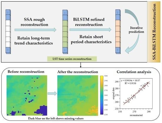
In this paper, an LST reconstruction method combining data decomposition and data prediction is proposed—SSA-BiLSTM. This method firstly performs rough LST data reconstruction by extracting the long-term features and change trends of the data using the SSA model and then complete refined LST data reconstruction by learning the short-term features of the data using the BiLSTM model. Experimental results prove the proposed method’s good performance and high robustness in LST reconstruction.
In
Section 2, the products and data used for analysis and the works related to data preprocessing are described. In
Section 3, the basic principles of SSA and BiLSTM are introduced, and the reconstruction method based on the SSA-BiLSTM model is described in detail. In
Section 4, the accuracy of the proposed method in LST reconstruction is analyzed qualitatively and quantitatively using remote sensing data and measured data. The advantages and disadvantages of the proposed method are summarized in
Section 5.
4. Results and Discussion
The accuracy of the method proposed in this paper was analyzed quantitatively and qualitatively using remote sensing data and measured data. In addition, the proposed method was compared with other three LST reconstruction methods, including the LST reconstruction method based on SSA, the LST reconstruction method based on SG filter, and the LST reconstruction method based on SSA-LSTM. The LST reconstruction method based on SSA relies on data decomposition and iterative prediction for LST reconstruction. The LST reconstruction method based on SG filter performs least squares data fitting using higher order polynomials and completes data reconstruction through a weighing filter. The only difference between the third and proposed method is in the size of predictive models used. The verification results indicate that the prediction results produced by the BiLSTM model are more accurate than those produced by the LSTM model.
4.1. Quantitative Analysis
Firstly, a comparative analysis was performed using the “removal–reconstruction–comparison” process to analyze the performance of various methods in LST reconstruction involving varying rates of missing data. The principle of this analysis method is to remove some existing data randomly from the complete time series, reconstruct the missing data using different reconstruction methods, and compare the original values of missing pixels with reconstructed data. Therefore, the LST data with 500 pixels in six consecutive years in the study area were randomly selected, some existing data were removed randomly to achieve missing rates of 10%, 20%, 30%, 40%, and 50%, and the results of LST reconstruction using the methods above were analyzed statistically (The statistical results of average accuracy are shown in
Figure 5). It can be seen from
Figure 5 that the proposed method is superior to other methods in terms of overall accuracy in LST reconstruction at varying missing rates. For the proposed method, the maximum coefficient of correlation between the original values of missing data points and reconstructed data is 0.9942, the minimum value of RMSE is 1.1069, and the minimum value of MAPE is 0.3210. The method based on SG filter has the lowest accuracy in LST reconstruction, its reconstruction error at 50% missing rate is more significant than 4 K, and its reconstruction accuracy is 2.4 K lower than that of the proposed method. In addition, a group of data are randomly selected from the above 500 pixels to analyze the correlation before and after reconstruction, so as to more clearly show the difference between the reconstructed LST data and the original value. The analysis results are shown in
Figure 6. It can be seen from figure that when the missing rate is high, compared to other methods, the correlation between the LST data reconstructed with the proposed method and the original data is the highest. In comparison, the correlation between the LST data reconstructed the LST reconstruction method based on SG filter and the original data is the lowest, and there are great differences at some missing data points before and after reconstruction.
The accuracy of the method proposed in this paper was further verified using the data measured at a number of weather stations. In
Section 2.2.2, the time consistency between the measured data of the meteorological station and the surface temperature data of MYD11A2 has been processed. Therefore, the measured data used in this experiment have 46 values every year. Firstly, 40% of the MODIS LST time series data were removed in 2020 at Yutian Station, Cele Station, Hotan Station, Luopu Station, Moyu Station, and Pishan Station, ensuring consistency of the times of missing values in each group of data. Then, LST data reconstruction was performed using the proposed method and other methods. There were 96 missing values in the data measured in 2020 at the six weather stations. The data measured at these weather stations corresponding to the times of missing values in 2020 were used to verify the accuracy of the proposed method. The correlation between the LST data reconstructed with this method and measured data were analyzed. The analysis results are shown in
Figure 7. It can be seen from
Figure 7 that the coefficient of correlation between the reconstructed data of the method in this paper and the data measured at weather stations is 0.9108, while the coefficient of correlation between the original data and measured data is 0.9231. These two values are basically consistent. In addition, it can be seen from the scatter plots of the original MODIS LST data measured after midnight and the reconstructed LST data with the proposed method that most data points before and after reconstruction are concentrated near the 1:1 line, which further proves the high accuracy of the proposed method.
4.2. Qualitative Analysis
In order to evaluate the performance of various LST reconstruction methods in a more visual way, the complete LST data of year 2020 within
pixel range were selected in the study area shown in
Figure 1 and used as the data for the experiments. Some existing data were removed randomly to create a missing rate of 40%. The areas with missing data were reconstructed using the four methods mentioned above.
Figure 8 shows the reconstruction effects of different methods when the surface temperature data are continuously missing in the time domain. It can be seen from
Figure 8 that the values of LST data reconstructed using the method based on SG filter are slightly higher. In practice, due to the influence of weather or external environment, there are some abrupt changes in the time series of surface temperature, such as the sudden drop of temperature. SG reconstruction method mainly uses the data before and after the missing point to reconstruct the missing pixel. When the data value before and after the missing point are large, the value reconstructed using SG will be higher than the original result. In addition, the reconstruction method based on SSA lacks the details of time series due to the complement based on the trend characteristics of the data, so the reconstruction results are not accurate enough. The images reconstructed using the two methods based on SSA-LSTM and SSA-BiLSTM are more consistent with the original images. Since the BiLSTM model can read data bidirectionally, it can learn more potential data features and predict results more accurately than SSA-LSTM.
The differences in the data reconstructed using different LST reconstruction methods and the original data were treated to demonstrate the performance of the proposed method in LST reconstruction in a more visual way. The results are shown in
Figure 9. It can be seen from
Figure 9 that the proposed method is accurate in LST reconstruction, while the images reconstructed using the method based on SG filter deviate greatly from the original images.
In order to verify the regional applicability of the proposed method, Wenchuan in the Sichuan province was selected as the validation area. A small range of
pixels were selected from the Wenchuan area, and all missing pixels in 2020 were reconstructed according to the method in this paper. The comparison effect before and after reconstruction is shown in
Figure 10. The figure shows the reconstruction effect of this method on this region in different seasons. It can be seen that the method in this paper can achieve the reconstruction of a large number of missing pixels, and the reconstructed images are complete.
4.3. Limitations of the Proposed Method
Although the proposed method can achieve relatively high accuracy in LST reconstruction when there are a large number of missing values in time series data, it has certain limitations. Firstly, the method in this paper lacks the use of spatial information. When further research is conducted in the future, consideration can be given to establishing a reconstruction model that combines a convolutional neural network with the predictive model to identify the spatial and temporal features of LST and achieve higher accuracy in LST reconstruction. Secondly, due to the significant impact of abrupt changes such as changes in weather conditions on LST reconstruction, the performance of the proposed method in reconstructing some pixels is unsatisfactory. In subsequent LST reconstruction efforts, more attention should be paid to data reconstruction problems caused by changes in weather conditions.
5. Conclusions
The large number of missing values in MODIS LST data restricts the use of such data. SSA-BiLSTM, an LST reconstruction method combing data decomposition with data prediction, is proposed to obtain spatially and temporally continuous LST data. This method consists of two major processes, namely, rough LST reconstruction based on the trend features of the data extracted using the SSA model and refined LST reconstruction based on the short-term features of the data learned by BiLSTM model.
A comparative analysis of the four methods mentioned in this paper is performed through “removal–reconstruction–comparison” using RMSE, R2, and MAPE based on remote sensing data and measured data. Experimental results show that when the missing rate is high, the deviations of data reconstructed using the methods based on SG filter and SSA are great, and the stability of reconstructed data is relatively low. Hybrid models based on data decomposition perform better than single models in LST reconstruction. The SSA-BiLSTM model is more accurate than the SSA-LSTM in LST reconstruction, indicating that compared with the latter, the former can consider the features of the entire time series data more adequately and perform better in predicting unknown data.


