Article

Multi-Scale Assessment of SMAP Level 3 and Level 4 Soil Moisture Products over the Soil Moisture Network within the ShanDian River (SMN-SDR) Basin, China

1
State Key Laboratory of Water Resources and Hydropower Engineering Science, Wuhan University, Wuhan 430072, China
2
School of Water Conservancy & Civil Engineering, Northeast Agricultural University, Harbin 150030, China
3
State Key Laboratory of Information Engineering in Surveying, Mapping and Remote Sensing, Wuhan University, Wuhan 430079, China
4
Key Lab of Ecosystem Network Observation and Modelling, Institute of Geographic Sciences and Natural Resources Research, Chinese Academy of Sciences, Beijing 100101, China
5
University of Chinese Academy of Sciences, Beijing 100049, China
6
Research Center of Fluid Machinery Engineering and Technology, Jiangsu University, Zhenjiang 212013, China
*
Author to whom correspondence should be addressed.
Remote Sens. 2022, 14(4), 982; https://doi.org/10.3390/rs14040982
Submission received: 5 January 2022 / Revised: 1 February 2022 / Accepted: 14 February 2022 / Published: 17 February 2022
(This article belongs to the Special Issue Remote Sensing of Soil Moisture for Agricultural Purposes)

Abstract

:
The Soil Moisture Active Passive (SMAP) mission with high-precision soil moisture (SM) retrieval products provides global daily composites of SM at 3, 9, and 36 km earth grids measured by L-band active and passive microwave sensors. The capability of passive microwave remote sensing has been recognized for the estimation of SM variations. The purpose of this work was to establish an interaction between the highly variable SM spatial distribution on the ground and the SMAP’s coarse resolution radiometer-based SM retrievals. In this work, SMAP Level 3 (L3) and Level 4 (L4) SM products are validated with in situ datasets observed from the different locations of the Soil Moisture Network within the ShanDian River (SMN-SDR) Basin over the period of January 2018 to December 2019. The values of the unbiased root mean square error (ubRMSE) for L3 (SPL3SMP_E) SM retrievals are close to the standard SMAP mission SM accuracy requirement of 0.04 m 3 / m 3 at the 9-km scale, with an averaged ubRMSE value of 0.041 m 3 / m 3 (0.050 m 3 / m 3 ) for descending (ascending) SM with the correlation (R) values of 0.62 (0.42) against the sparse network sites. The L4 (SPL4SMGP) Surface and Root-zone SM (RZSM) estimates show less error (ubRMSE < 0.04) and high correlation (R > 0.60) values, and are consistent with the previous SMAP-based SM estimations. The SMAP L4 SM products (SPL4SMGP) performed well compared to the L3 SM retrieval products (SPL3SMP_E). In vegetated land, the variability and compatibility of the SMAP SM estimates with the evaluation metrics for both products (L3 and L4) showed a good performance in the grassland, then in the farmland, and worst in the woodlands. Finally, SMAP algorithm parameters sensitivity analysis of the satellite products was conducted to produce time-series and highly precise SM datasets in China.

Graphical Abstract

1. Introduction

Soil moisture, a most active key variable, interrelates the processes of Earth’s energy and water between the atmosphere and land surface, and plays a vital role in hydrological processes [1,2], bio-geochemical processes, bio-ecological processes, and crop yield estimation [3]. The estimation of SM with high accuracy and fine spatio-temporal resolution is useful for modelling and forecasting weather and climate [4] and monitoring floods and droughts [5,6]. In general, the traditional method for determining the SM content requires reasonably precise ground assessments at a point scale utilizing site networks [7,8], such as the United States Department of Agriculture (USDA) and Soil Climate Analysis Network (SCAN) throughout the United States. The distribution of surface soil moisture (SSM) on a regional or global scale is difficult to identify due to the lack of sufficient ground measurement sites in many places. Due to the advantages of remotely sensed data, several attempts have been made to estimate SSM for regional or even worldwide applications.
At a large spatial scale with a high temporal resolution, microwave remote sensing provides near-SSM datasets with relatively high accuracy. Using remote sensing, Jackson and Schmugge have come up with a novel approach for obtaining SSM. The SMAP [9], developed by National Aeronautics Space Agency (NASA), launched on 31 January 2015, providing high-resolution soil SM moisture and freeze/thaw datasets at 2–3-day intervals with a 36, 9, and 3-km earth grid estimated by active and passive microwave sensors. The SMAP satellite is equipped with an L-band radar (1.26 GHz) and an L-band radiometer (1.41 GHz) that deliver backscatter observations at a spatial resolution of 3 km and brightness temperature (TB) measurements at a 36 km resolution [10], respectively. The L-band microwaves estimation, because of a significant penetration ability, has been considered the most appropriate band for SM assessment, especially in high-density vegetative regions. These estimations are likely more sensitive to SSM and temperature, which influence the land surface water (conversion of precipitation into runoff, infiltration, and evaporation) and energy balance (partitioning of incident radiations into sensible and latent heat fluxes) [11,12]. Unfortunately, the L-band radar (active) failed on 7 July 2015 due to some mechanical issues, but the L-band radiometer (passive) is providing global imagery of SM. There are 4 different levels of SMAP data products containing Level 1 datasets (raw and/or calibrated instruments calculations), and Level 2, 3, and 4 products for SM observations are being delivered. In the present study, L3 and L4 SMAP products were used for SM retrieval over the period of 1 January 2018 to 3 December 2019.
SMAP L3 products offer daily global-scale aggregates of half-orbit SM based on Level 2 observational data. The SMAP L3 36-km daily global composite radiometer SM (L3 SM P) and 9-km enhanced daily global composite radiometer SM (L3 SM P E) datasets are widely utilized. Xu [13] worked with the 36-km radiometer product SPL3SMP_E a.m. (descending half-orbits with a local solar time of 6 a.m.) and estimated the ubRMSE close to 0.014 m 3 / m 3 , with R and anomaly R values of more than 0.65. Against the sparse observation network, the average ubRMSE value was ~0.06 m 3 / m 3 , with R and anomaly R values of close to 0.50, and concluded that SPL3SMP_E p.m. (ascending half-orbits with a local solar time of 6 p.m.) values slightly underestimated the a.m. SM truths. In the Little Washita Watershed (LWW) network in the United States, Cui et al. [14] tested a 9-km L3 SM P E a.m. (ver-1) SM with ubRMSE less than 0.04 m 3 / m 3 and a significant correlation coefficient greater than 0.87.
SMAP L4 products are obtained by assimilating TB data from SMAP datasets into the land surface model (LSM). The L4 SM algorithm is based on the GEOS-5 Catchment LSM and is a modified version of the ensemble-based Goddard Earth Observing System (GEOS-5) LDAS (Land Data Assimilation Systems) [15,16]. The SMAP L1C TB and surface meteorological controlling inputs from the GEOS-5 atmospheric assimilation system, calibrated with rainfall data, are the principal drivers of this system. A spatially distributed ensemble Kalman filter is being used to merge SMAP TB estimations with model-driven estimates [17,18]. The averaged geophysical SM data for both the surface (0–5 cm) and the root-zone (0–100 cm) depths are provided at 3-h intervals in SMAP L4 products (SPL4SMGP) at a 9-km global cylindrical Equal-Area Scalable Earth (EASE) Grid projection [13].
The implementation of SMAP SM products and the refinement of the retrieval algorithm both require their validation. Previously, for the validation of remotely sensed SM, a lot of work has been conducted in the Tibetan Plateau, China [19,20,21,22,23,24,25,26,27]. For calibration and validation of SMAP radiometric datasets, different complementary methodologies are being used to improve the accuracy and performance of the SMAP mission and to achieve global robust SM assessment. These methodologies comprise core validation measurements [28], sparse network [29,30], model-derived products [31,32,33], other satellites datasets [34], and field operations [35,36]. This study used core validation measurements (containing all the sites within the SMAP grid-cell) and sparse network (containing one in situ station within the SMAP resolution cell) to match in situ SM with SMAP-derived SM. The application of multi-scale validation approaches provides information on the reliability of remote sensing data and consistency with in situ measurements at any scale.
The SMAP SM retrieval algorithm is affected by a wide range of parameters, including the surface temperature, vegetation, and surface roughness [37]. These perturbing factors disturb the interaction between TB and SM, resulting in uncertainties in the SM estimates. The emitted energy from soil is significantly influenced by the vegetation canopy. The vegetation canopy scatters and absorbs microwave emissions from the soil while simultaneously emitting its own. This scattering, absorption, and emission are caused mainly by the water retained inside the canopy. In addition to attenuating radiation emitted by soil surfaces, vegetation reduces the brightness temperature’s sensitivity to SM [38]. SMAP SM measurements are based on soil’s dielectric characteristics, which vary with SM and are influenced by the soil temperature [39]. Lu et al. [40] revealed that variations in SM are related to changes in the soil temperature and are mostly driven by temperature effects. They developed a real-time method for effectively removing temperature impacts from soil water.
The present work evaluated the SMAP SM products over the ShanDian River Basin, utilizing in situ data acquired by the SMN-SDR network. This study focused on achieving the following purposes: (1) to validate the SMAP SM products across the humid area (SMN-SDR) of the North China Plain, over the period of 1 January, 2018 to 31 December, 2019, to provide practical implementation assistance in the region; (2) to evaluate the L3 and L4 SMAP SM products (SPL3SMP_E and SPL4SMGP) compared with in situ observations; and (3) to evaluate SMAP SM L3 and L4 products across the SMN-SDR Basin under different vegetation types and spatio-temporal scales. This paper is organized as follows: Section 2 describes the SMAP SM products and in situ datasets. Section 3 provides a comprehensive assessment of the SMAP SM products based on in situ measurements. The results are discussed in Section 4, followed by the conclusions of this study, which are described in Section 5.

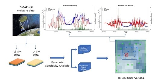
2. Materials and Methods

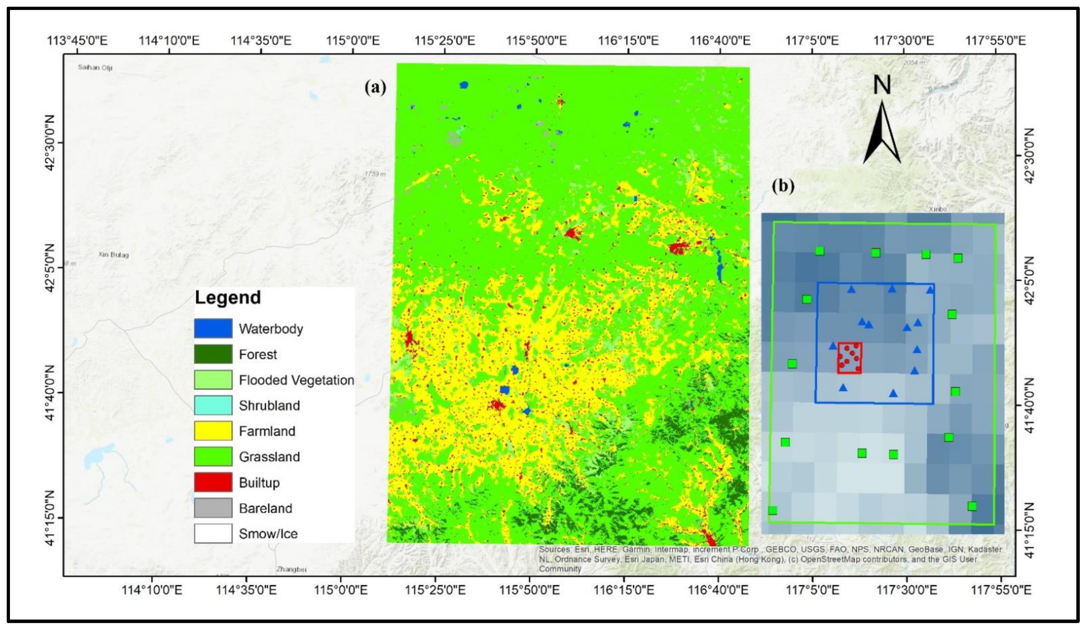
2.1. Study Domain and Ground Observation Network and Datasets

This work acquired ground-based SM data from a wireless Soil Moisture Network within the ShanDian River Basin, referred to as SMN-SDR, in the North China region. During the SM experiment in the Luan River, the SMN-SDR was established from 18 July 2018 to 28 September 2018 [40]. The in situ SM data for the SMN-SDR network was available in the International Soil Moisture Network (ISMN) [7]. The area coverage of the entire network is 10,000 km2 (115.5–116.5° E, 41.5–42.5° N). A total of 34 stations comprised the network, which was built up with 3 sample scales, including large-scale (100 km), medium-scale (50 km), and small-scale (10 km) samples, as described in Table 1. The large-scale (L) stations have an M-shaped layout, medium-scale (M) stations have a plum-shaped layout, and small-scale (S) stations are exactly within the SMAP 9-km grid as shown in Figure 1. Decagon EM50, USA (5TM probes) sensors were used for each station to estimate SM at 5 measuring depths (3, 5, 10, 20, and 50 cm). The data recording time period was 10 and 15 min (before and after June 2019). The geography of the SMN-SDR is rather flat, and the land surfaces are mostly covered by farmland and grassland, with a few patches of forest and wetlands. Table 1 summarizes the detailed information about each site in the SMN-SDR, including the station ID, latitude, longitude, elevation, setup time, and land use type.
The SMN-SDR encompasses multi-layer soil temperature (at the same depths of the SMs) and other meteorological variables, e.g., precipitation. In total, 20 stations out of 34 are equipped with HOBO rain gauges (made by Austria), which can record up to 160 inches of rain at rates of up to 12.7 cm (5 inches) per hour in the SMN-SDR. These stations are mostly located on small and medium scales. Detailed information about the HOBO rain gauge can be found at https://www.onsetcomp.com/products/data-loggers/rg3/, last accessed: 3 February 2022. All these stations provide time serial SM, soil temperature, and precipitation on an hourly basis. The experimental region has a moderate continental climate, with annual precipitation ranging from 300 to 500 mm in most regions, with 70% of the precipitation occurring between July and September [40]. Snowmelt in March and April frequently causes a modest spring flood. The SMN-SDR has a generally flat terrain, with grasslands and croplands dominating land surfaces.
The data sets recorded from the sensors (5 TM and HOBO) only include raw data. SM data obtained from sensor 5TM was calibrated using the following equation [40]:
SMC V = 1.0458   ×   SMC 5 TM 0.0022
where SMC V is the calibrated soil moisture (% volume) and SMC 5 TM is the actual SM recorded by the 5TM sensor (% volume).
The 5TM sensor’s accuracy and resolution for SM are ±3% m 3 / m 3 and 0.0008 m 3 / m 3 , and for soil temperature, ± 1 K and 0.1 K, respectively. After laboratory examination, the SMN-SDR in situ SM data was already calibrated and validated with ground truth SM data taken from different soil samples at each layer [40]. In this research work, the SMN-SDR SM data at 5-cm depths (over the period 25 July 2018 to 31 December 2019) were used to validate L3 SMAP_E and L4 SMAP_GAU (SSM) data, and 50 cm to validate Level 4 SMAP_GAU (RZSM) data.

2.2. SMAP Soil Moisture Products

The SMAP captures the global brightness temperature (TB) with a spatial resolution of 36 km and a temporal resolution of 3 days. The SMAP satellite is equipped with an L-band radar (active) and L-band radiometer (passive) for monitoring the Earth’s surface at sun-synchronized times of 06:00 a.m. (descending) and 06:00 p.m. (ascending) [41]. The radar and radiometer started providing SMAP imaginary on 31 March and 13 April 2015, respectively. Radiometer (passive) devices are less susceptible to vegetation intensity and ground surface roughness than radar (active) instruments, although the high spatial resolution of radars (about 1–3 km) is not equivalent to the radiometer’s moderate resolution (around 40 km). The combination of radar and radiometer sensors in SMAP increases SM measurement’s accuracy and spatial resolution [42]. However, on 7 July 2017, the radar stopped providing SMAP active microwave datasets due to mechanical failure. Through radiometric-based techniques [43], the near-SSM (0–5 cm) are estimated with a 0.04 m 3 / m 3 volumetric accuracy. The NSIDC website (https://www.nsidc.org/data/smap/smap-data.html, last accessed: 5 January 2022) provides free access to all datasets. In this research work, we evaluated 2 SMAP SM products: Level 3 enhanced SMAP radiometric SM (SPL3SMP_E) at a global daily 9-km EASE-Grid spatial resolution, version 4 [30]; and Level 4 SMAP SSM and RZSM (SPL4SMGP) at a global 3-hourly 9-km EASE-Grid spatial resolution, version 5 [44]. These two SMAP products are briefly demonstrated here.
The SPL3SMP E products are enhanced Level 3 radiometric (passive) SSM retrieval products based on enhanced Level 2 SMAP products [45], which provide daily global SSM (5 cm depth) estimates from SMAP 6:00 a.m. (descending half-orbits) and 6:00 p.m. (ascending half-orbits) TB datasets, respectively [30]. The SPL3SMP E datasets, which have an EASE-Grid 2.0 resolution of 9 km, provide 1–3 days of the average temporal resolution for half-orbit fields. The SPL4SMGP product was obtained from SMAP L-band TB data using the EnKF assimilation technique in the Catchment LSM [46]. The LSMs have an excellent capability to convert water (in the form of precipitation) into runoff, evaporation, and storage estimations, and energy (in the form of incoming radiations) conversion into latent heat, sensible heat, departing radiations, and other various terms [44]. The SPL4SMGP product (version 5) provides instantaneous SM at 3-hourly time-averaged from assimilation system, 9-km Global cylindrical EASE-Grid 2.0 for both layers, surface (0–5 cm), and root-zone (0–100 cm). In this work, we utilized the SPL4SMGP datasets for SSM and RZSM retrieval from geophysical data.
The present study used the SPL3SMP_E products and SPL4SMGP datasets for SM estimation from January 2018 to December 2019. The SPL3SMP_E products containing adverse climatic conditions (snow cover, frozen surfaces, urban, open water, etc.) were already excluded.

2.3. Statistical Analysis

The SMAP SM products were qualitatively evaluated with the SMN-SDR network at 2 spatial scales: core validation sites (CVSs), which provide all of the S-scale (S) stations that exist within an SMAP product grid-cell with a 9-km resolution; and a sparse network of M-scale (M) and L-scale (L) stations, which provides a point-scale measurement containing only 1 station within an SMAP product grid-cell (9-km). In this study, these networks were utilized to compare the SMAP SM products with a 9-km spatial resolution (SPL3SMP_E and SPL4SMGP) using a series of statistical metrics, including the unbiased root mean square error (ubRMSE) [47,48], correlation coefficient (R), anomaly R [49], and mean bias [24]. The validating metrics are defined as follows:
Bias   =   E [ θ   e s t ] E [ θ   i n s i t u ]
RMSE   =   E [ ( ( θ   e s t ) ( θ   i n s i t u ) ) 2 ]
ubRMSE   =   E [ ( ( θ   e s t E [ θ   e s t ] ) ( θ   i n s i t u E [ θ   i n s i t u ] ) ) 2 ]  
R = E [ ( θ   e s t E [ θ   e s t ] ) ( θ   i n s i t u E [ θ   i n s i t u ] ) ]   ( σ   e s t σ   i n s i t u ) 1
where E [.] is the expectation value operator. θ   e s t and   θ   i n s i t u represent SMAP and in situ SM values, respectively.   σ   e s t is the standard deviation of θ   e s t and σ   i n s i t u is the standard deviation of θ   i n s i t u .
The evaluation metrics for SPL3SMP_E and SPL4SMGP SSM estimations were validated with in situ SMN-SDR network topsoil layer (0–5 cm) measurements. SPL4SMGP RZSM was evaluated by taking the arithmetic mean of SMN-SDR network observations in the up to 50 cm soil layer. It is recognized that the soil depths for SMAP datasets do not correspond properly with the sensor depths for the in situ observations. However, using limited in situ measurements in the study region, we demonstrated that the depth variation across SMAP products has only a minimal impact on the evaluation.

3. Results

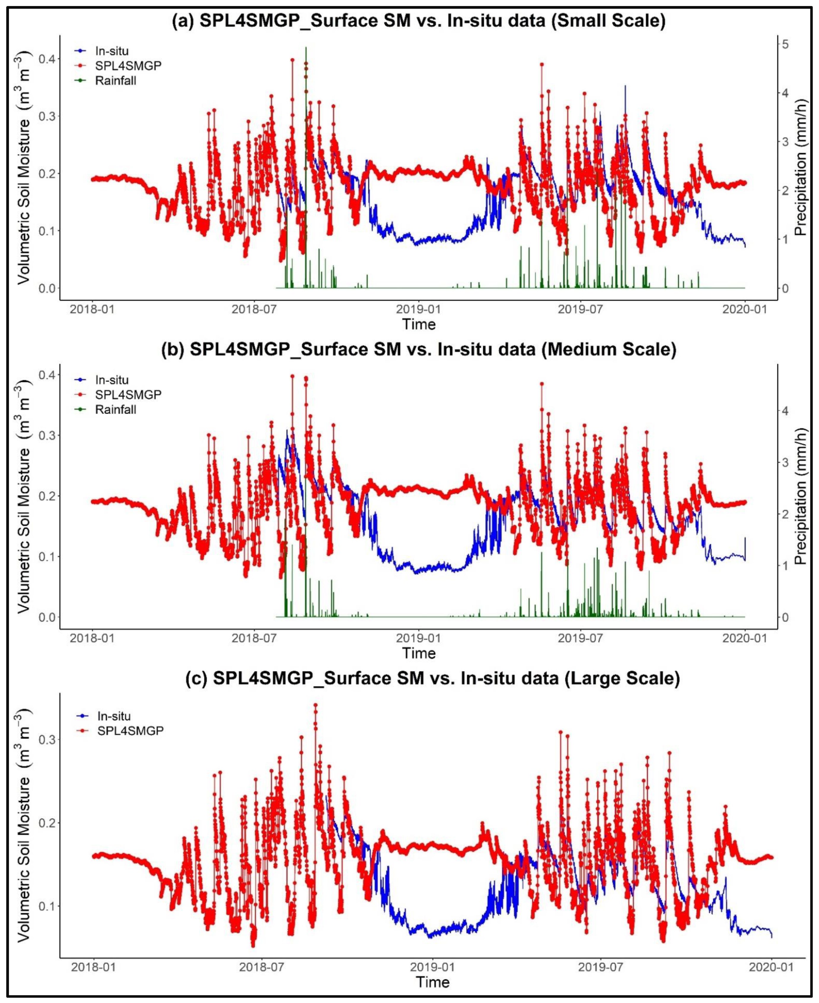
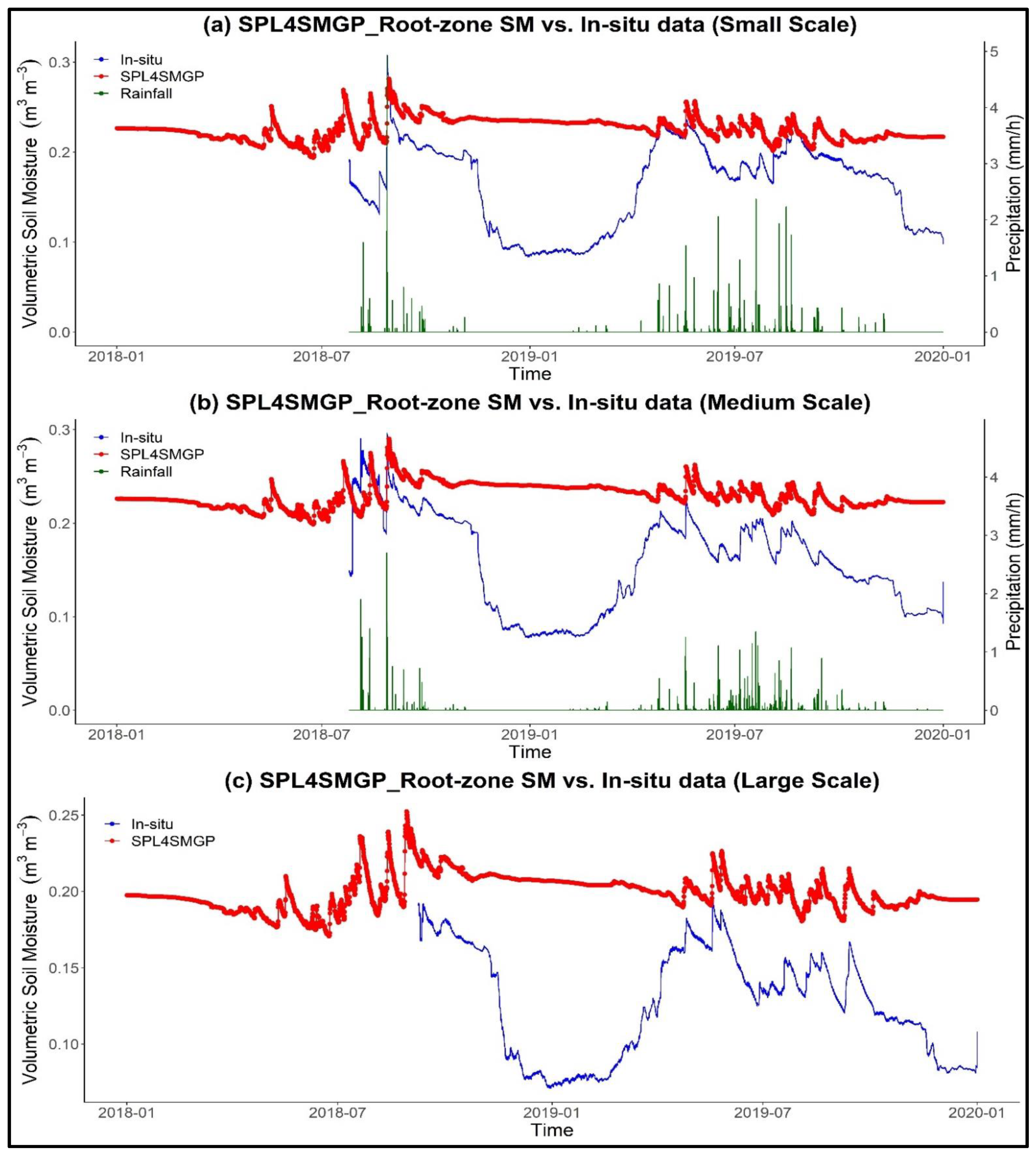
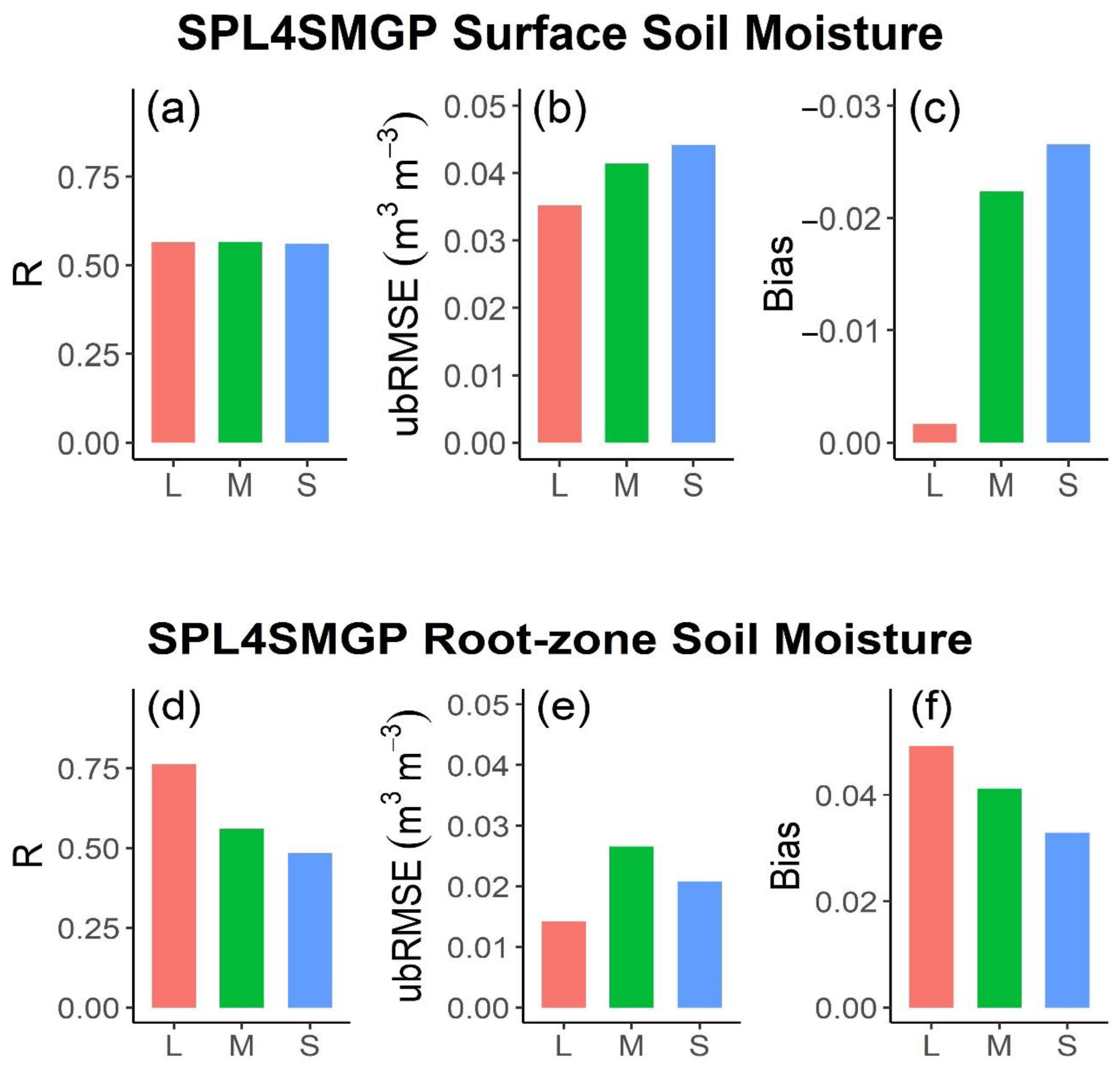
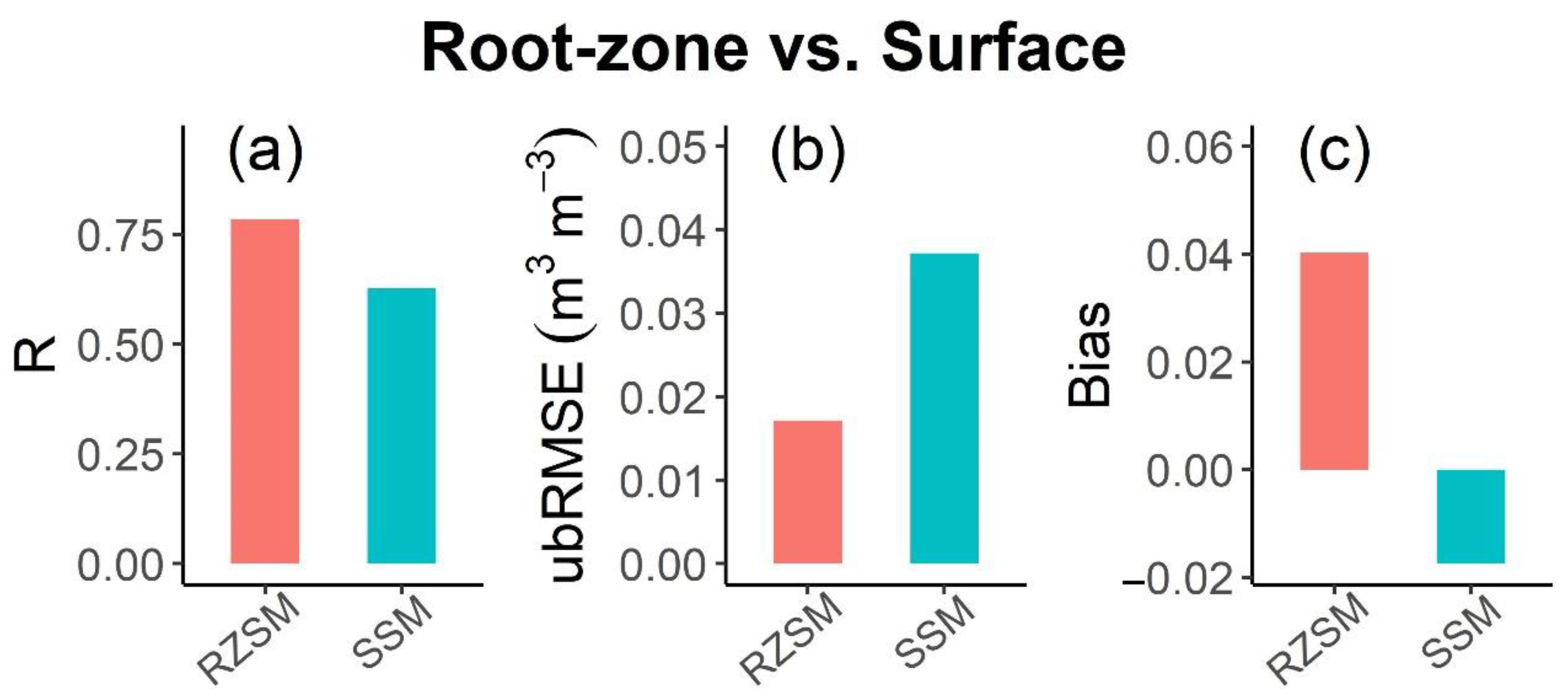
3.1. Evaluation of the SPL4SMGP Surface and Root-Zone Soil Moisture

This section analyzes and discusses the performance of the SPL4SMGP SSM and RZSM products over three different scale sites. We compared the temporal variations of SPL4SMGP SM with in situ data at different spatial locations (i.e., small, medium, large), as shown in Figure 2 and Figure 3. The performance metrics of all the spatial locations (S, M, and L) are described in Figure 4. These metrics were calculated from the 3-hourly SPL4SMGP SSM and RZSM and 3-hourly composites of in situ SM from 25 July 2018 to 31 December 2019. At the S-scale, a total of eight ground sites located within the SMAP radiometric pixels (as a core validation site) were used for the evaluation of SPL4SMGP SM. The time-series validation results of SPL4SMGP SSM and RZSM with in situ SM for S-scale sites are shown in Figure 2a and Figure 3a. At M and L scales, 12 and 14 in situ sites, respectively, were used to evaluate SMAP SM as the sparse network sites. The SPL4SMGP SSM and RZSM and in situ SM estimates showed almost a constant value from November 2018 to March 2019. This is due to snowfall events that occurred in the study area during the same time period. SMAP TB estimates were unavailable in the winter because of frozen states; hence, the L4 product estimations are only based on the results of the GEOS-5 model simulations [50], resulting in a linear time series trend for the L4 products in winter (as shown in Figure 2 and Figure 3).
The SPL4SMGP SSM estimates were underestimated with a bias of −0.026 m 3 / m 3 relative to the in situ SM. In contrast, SPL4SMGP RZSM retrievals had a positive bias of 0.033 m 3 / m 3 , indicating an overestimation compared to the in situ observations. The RMSE values are 0.051 m 3 / m 3 and 0.038 m 3 / m 3 for the SSM and RZSM datasets, respectively. After removing their respective biases from RMSE, a moderate to good accuracy was obtained, with ubRMSE values of 0.044 m 3 / m 3 with a standard deviation value of 0.052 m 3 / m 3 for the SPL4SMGP SSM and 0.20 m 3 / m 3 with a lesser standard variation of around 0.013 m 3 / m 3 for the SPL4SMGP RZSM. The SPL4SMGP SSM products showed a good correlation value of 0.57 compared to 0.48 for the SPL4SMGP RZSM products. At the medium scale (M), ubRMSE values of 0.045 m 3 / m 3 and 0.026 m 3 / m 3 were obtained after removing the corresponding biases values of −0.022 m 3 / m 3 and 0.041 m 3 / m 3 , which occurred in the observations, from the relative RMSE values of 0.057 m 3 / m 3 and 0.056 m 3 / m 3 for the SPL4SMGP SSM and RZSM datasets, respectively, as shown in Figure 4. The SPL4SMGP RZSM showed a lower error with a higher correlation value of 0.056 m 3 / m 3 (Figure 4a,d) for both the SPL4SMGP SSM and RZSM due to less variability during the time period. Next, for L-scale, the SPL4SMGP RZSM products revealed a much better correlation of 0.76 and high accuracy (ubRMSE = 0.014 m 3 / m 3 ) as compared to SSM (R = 0.56, ubRMSE = 0.041 m 3 / m 3 ) (Figure 4). We observed that the SPL4SMGP SM datasets over the sparse network (M and L scales) showed better results than the core validation site (S scale).
In the end, the averaged ubRMSE value of all the in situ stations for RZSM (0.017 m 3 / m 3 ) was considerably lower than that of the SSM value (0.037 m 3 / m 3 ) (Figure 5b). As previously stated, this was simply due to the lower temporal variability in RZSM. The correlation values for the SPL4SMGP SSM (R = 0.78) and RZSM (R = 0.63) datasets were significantly higher than that of other spatial scale stations, as shown in Figure 5a. The overall performance metrics are shown in Figure 4 for the spatial sites. For both SPL4SMGP SSM (except the S- and M-scale stations) and RZSM products, all the spatial scale stations met the product’s accuracy requirements (ubRMSE value less than 0.04 m 3 / m 3 ).

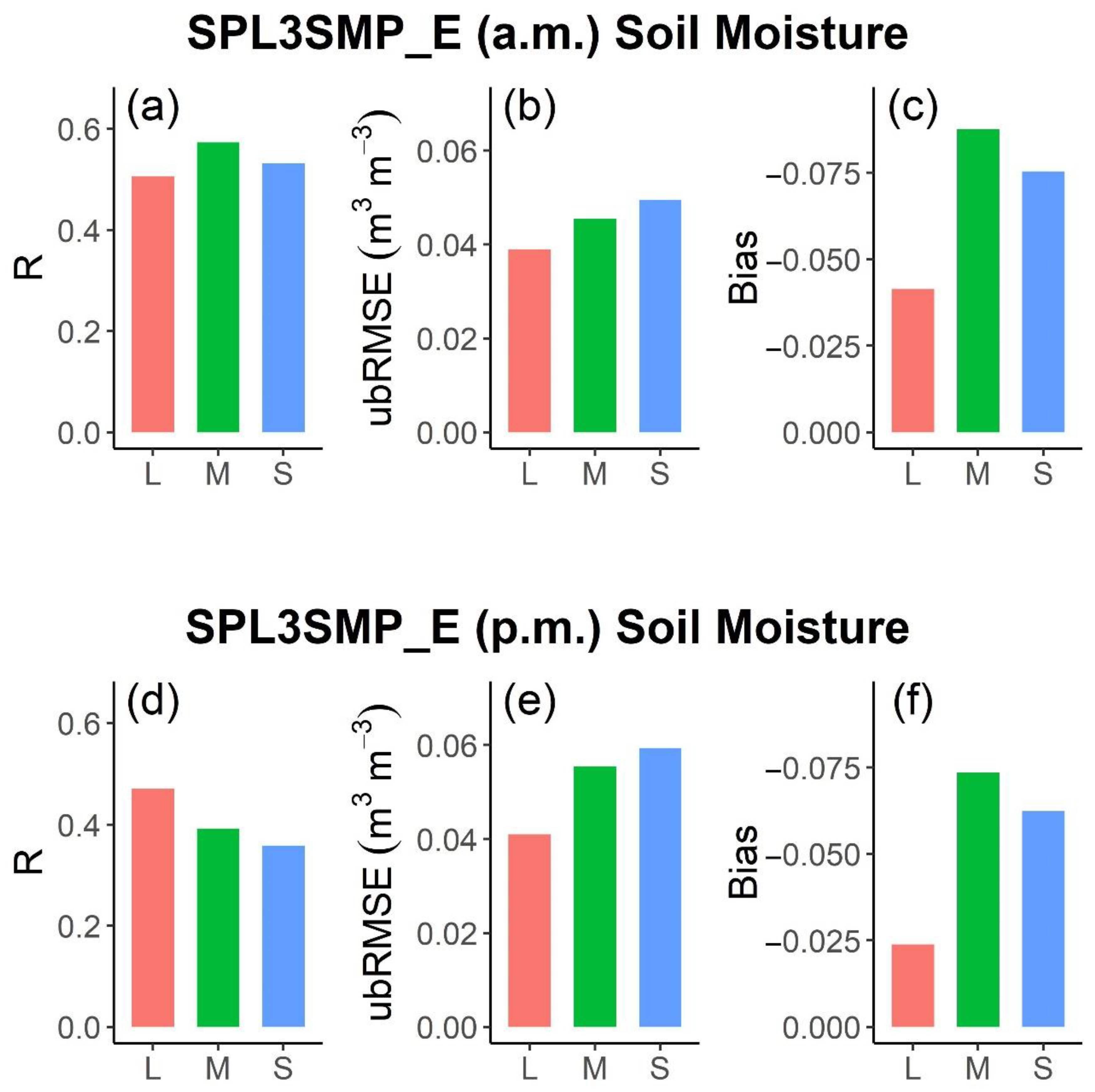
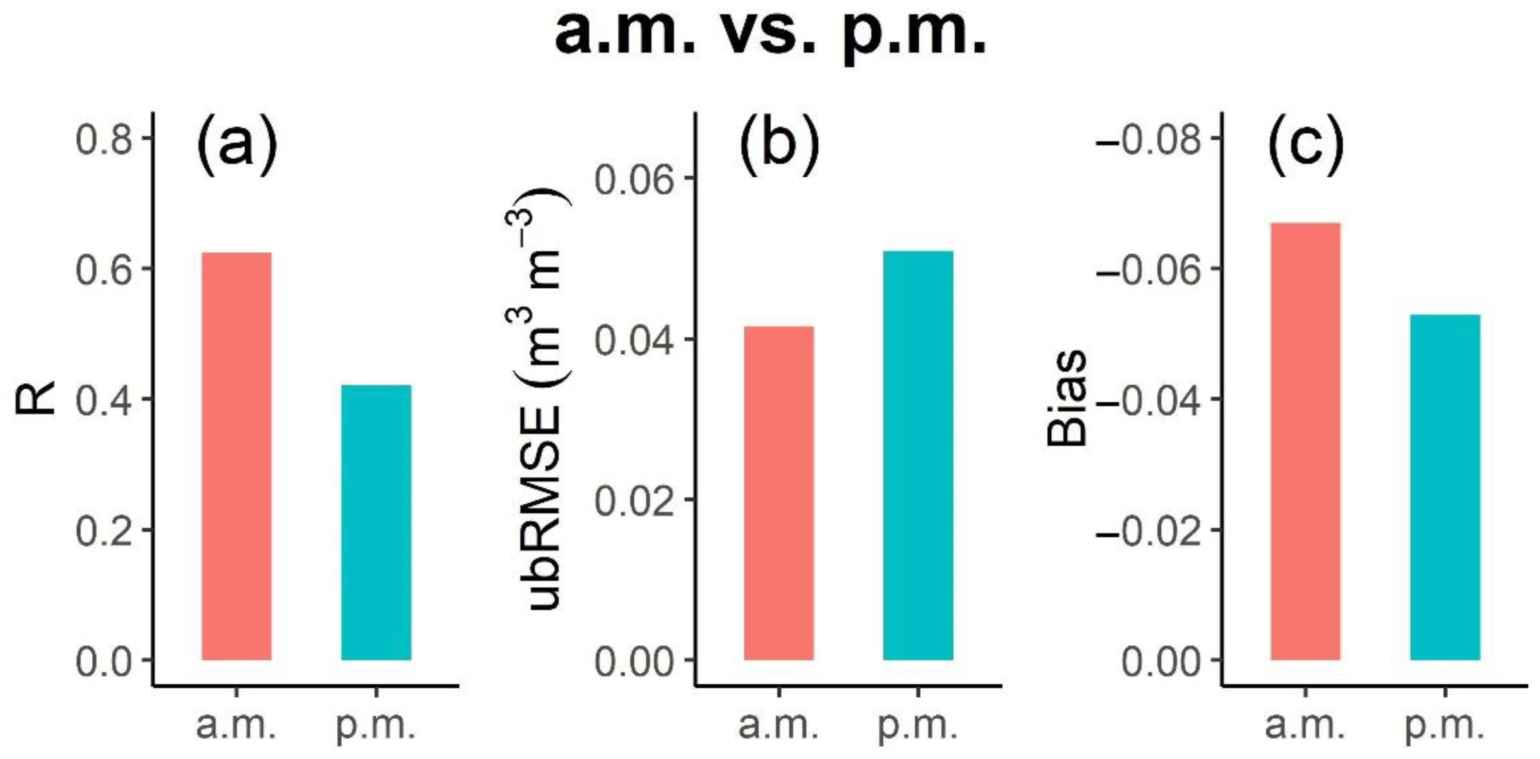
3.2. Evaluation of SPL3SMP_E Ascending and Descending SM

We first presented the SPL3SMP_E a.m. (descending) and SPL3SMP_E p.m. (ascending) SM validation at different spatial locations (S, M, and L). Figure 6 and Figure 7 show a time series evaluation of SPL3SMP_E SM with an hourly composite of in situ SM at core validation sites (S) to a sparse network of validation sites (M and L). No data from the SPL3SMP_E a.m. and p.m. SM products in winter was available because of seasonal snowfall events in the study area. In the SMAP mission, the relationship between SM and the dielectric constant is used to derive SM data. A rise in the dielectric constant is associated with an increase in the soil reflectivity and emissivity, which may either increase or decrease depending on the value of SM [43]. However, frozen soil contains a low dielectric constant similar to the dry soil dielectric constant regardless of the water content [51]. The error metrics (i.e., R, ubRMSE, bias) are presented in Figure 8 and Figure 9. These error metrics were calculated from daily composites of SPL3SMP_E a.m. and p.m. SM compared with the reference daily composites of in situ SM at 6 a.m. Local Standard Time (LST) and 6 p.m. LST, respectively, for 25 July 2018 to 31 December 2019.
Figure 6a shows a temporal validation between SPL3SMP_E a.m. SM and hourly composites of in situ SM at S-scale sites as core validation. Figure 6b,c show a time series validation representation of SPL3SMP_E a.m. estimations with in situ SM at the M-scale and L-scale. The SPL3SMP_E a.m. SM datasets showed good evaluation results corresponding to the rainfall events. At all spatial sites, the SPL3SMP_E a.m. retrievals contained ubRMSE values ranging from 0.038 m 3 / m 3 to 0.049 m 3 / m 3 , with a range of bias values from −0.04 m 3 / m 3 to −0.08 m 3 / m 3 (Figure 8), indicating that the sparse network sites showed good validation results as compared to the core validation sites. The RMSE values for a.m. retrievals (0.09 m 3 / m 3 ) are larger than for p.m. retrievals (0.08 m 3 / m 3 ), with biases of −0.075 m 3 / m 3 and −0.062 m 3 / m 3 for the a.m. and p.m. estimates, respectively (Figure 8). The M-scale sites showed good correlations values of 0.57, which are larger than that of the S-scale and large L-scale sites (R = 0.53, R = 0.50) for the ascending SPL3SMP_E SM datasets. Figure 7 shows a comparison of SPL3SMP_E p.m. (descending) SM retrievals with the in situ SM observations at different spatial locations (S, M, and L). The ubRMSE values for the S-, M-, and L-scale locations were 0.059 m 3 / m 3 , 0.055 m 3 / m 3 , and 0.043 m 3 / m 3 , respectively, which are comparatively larger than the SPL3SMP_E a.m. products, as shown in Figure 8. The time series SPL3SMP_E p.m. SM presented lower correlation (R) values than 0.50 for all locations. Because a.m. (night-time) retrievals are less susceptible to inaccuracies in land surface temperature estimations than p.m. (day-time) retrievals, the SPL3SMP_E a.m. estimations were more reflective of SM variability than the p.m. retrievals.
The SPL3SMP_E SM products performed better for sparse network sites (M and L) than core sites (S), reflecting vegetation cover’s adverse influence over satellite SM observations. In terms of precipitation, both ground observations and the SMAP SM products retrievals are capable of capturing precipitation events and SM variability trends. However, ground observations at various footprints reveal significant variations, but the SMAP SM datasets show only minor differences, as shown in Figure 6a,b and Figure 7a,b.
Figure 9 shows a comparison of the averaged evaluation metrics of SPL3SMP_E (a.m. and p.m.) SM estimations at all the 34 spatial validation locations (S, M, and L). The SPL3SMP_E a.m. SM estimates contained the averaged ubRMSE value of 0.041 m 3 / m 3 , which is much closer to the targeted value (ubRMSE = 0.04 m 3 / m 3 ), with bias values of −0.066 m 3 / m 3   (Figure 9b,c). In contrast, SPL3SMP_E p.m. SM estimates showed less accuracy and contained larger errors (ubRMSE = 0.050 m 3 / m 3 ), with a biasness value of −0.052 m 3 / m 3 . Overall, the correlation value for SPL3SMP E a.m. SM retrievals was more than 0.60 when compared to SPL3SMP E p.m. SM retrievals.

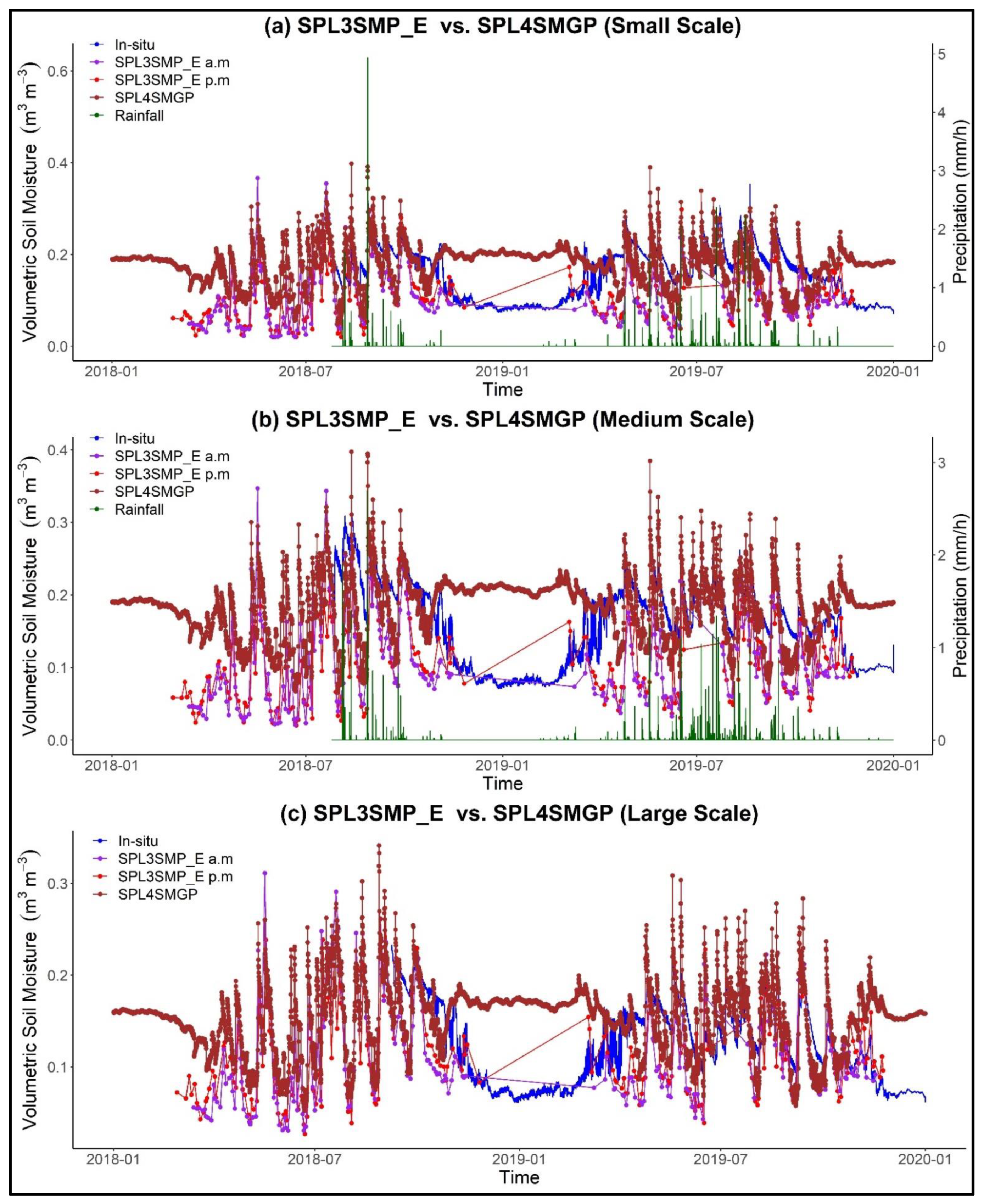
3.3. Comparison of SPL3SMP_E and SPL4SMGP Surface Soil Moisture

Figure 10 shows the comparison of SPL3SMP_E (a.m. and p.m.) and SPL4SMGP SSM estimates at all the spatial locations. The daily composites of SPL4SMGP SSM were constructed using 3-hourly data. At 6 a.m. and 6 p.m. (LST), daily composites of the closest 3-hourly data were created using SPL4SMGP SSM and compared to SPL3SMP_E a.m. and p.m. SM estimates. SPL3SMP_E (descending and ascending) SM estimations and SPL4SMGP SSM daily composites of the closest 3-hourly data at 6 a.m. LST and 6 p.m. LST were used to construct the average error metrics. At S-scale sites, the performance errors (R, ubRMSE, and bias) for both of SPL3SMP_E a.m. SM estimates (0.53, 0.049 m 3 / m 3 , and −0.07 m 3 / m 3 ) and SPL4SMGP SSM retrievals (0.56, 0.44 m 3 / m 3 , and −0.02 m 3 / m 3 ) are better than SPL3SMP_E p.m. SM estimates (0.35, 0.059 m 3 / m 3 , and −0.06 m 3 / m 3 ) as shown in Figure 11. At M and L scales (as the sparse network), the evaluation metrics for SPL3SMP_E a.m. SM estimates and SPL4SMGP SSM retrievals also performed better than SPL3SMP_E p.m. SM estimates (Figure 11).
The SPL4SMGP SSM retrievals showed better results related to the time series in situ SM measurements containing the lowest error ubRMSE, ranging from 0.044 m 3 / m 3 to 0.035 m 3 / m 3 , and a higher range of correlation values of 0.56 to 0.62, as compared to the other SPL3SMP_E (ascending and descending) SM products for all the spatial locations (S, M, and L), as shown in Figure 11. This reveals the improvements of the SMAP assimilation datasets (SPL4SMGP) over the satellite-only products (SPL3SMP_E). The integration of satellite-based SM and LSM, using data assimilation techniques, produces optimized results better than that of a single source of information (satellite/modeling). The SPL3SMP_E a.m. time series SM retrievals showed better results than the SPL3SMP_E p.m. SM estimates. Both the SPL3SMP_E a.m. and SPL4SMGP SSM datasets performed well in all the locations, especially in sparse network sites, and almost met the standard ubRMSE value of 0.040 m 3 / m 3 at most of the sites. Overall, it was observed that all the SMAP SM products performed well at the sparse network sites (M, L) compared to core validation sites (S).

3.4. Performance Assessment of the SMAP SM L3 and L4 Products under Various Vegetation Types

Different vegetation covers affect SMAP SM estimations. In this part, we compared the in situ SM estimations with the SM estimates from the SMAP L3 and L4 datasets under different vegetation types. As shown in Table 2, the R values for the L3 a.m. (p.m.) SM products ranged from 0.25 to 0.43 (0.08 to 0.48) under various vegetation types. The negative bias in the L3 datasets implies a dry bias for all types of vegetation. The RMSE values ranged from 0.06 to 0.09 m 3 / m 3 for L3 a.m. products and from 0.065 to 0.076 m 3 / m 3 for L3 p.m. products while the ubRMSE values for a.m. (p.m.) products ranged from 0.052 to 0.058 m 3 / m 3 (0.046 to 0.065 m 3 / m 3 ) under different vegetation covers. The L3 SM products did not achieve the standard accuracy of 0.04 m 3 / m 3 for all types of vegetation, especially in the woodlands of the study region.
The L4 product contains the R values for SSM (RZSM) products, which ranged from 0.20 to 0.44 (0.26 to 0.70), while the RMSE values ranged from 0.050 to 0.065 m 3 / m 3 (0.040 to 0.105 m 3 / m 3 ) with the positive bias values (except grassland) under all vegetation types. The ubRMSE is the major index for the assessment of SMAP SM between various vegetation types. The L4 SSM product shows that the ubRMSE values ranged from 0.044 to 0.051 m 3 / m 3 and for RZSM product, it ranged from 0.018 to 0.033 m 3 / m 3 , as shown in Table 2. The L4 RZSM product showed a better performance, containing ubRMSE values less than the standard accuracy of 0.04 m 3 / m 3 , with good correlation values of more than 0.60 (except farmland) for all vegetation types.
Overall, the L3 and L4 SM datasets performed better, with large R values and better ubRMSE values in grassland then farmland and woodland.

4. Discussion

In this paper, the SMAP SM products were evaluated with in situ SM observations at different soil depths for the area of the SM Network within the ShanDian River (SMN-SDR) Basin, and the corresponding results are explained in Section 3. The in situ SM data available at different soil depths (5 and 50 cm) was used for SMAP SSM and RZSM evaluation over the period of 25 July 2018 to 31 December 2019. The eight S-scale (S) stations, 12 M-scale (M) stations, and 14 L-scale (L) stations were used for this purpose. The overall performance of the SMAP SM products is discussed according to some aspects and compared with some previous studies. After launching the SMAP mission in 2015, SM estimation using remote sensing data became a hot research topic, especially in humid areas, which have been the least explored regions in this regard. In the present study, the SMAP L3 and L4 SM datasets were evaluated at different locations in the SMN-SDR Basin.
The SPL4SMGP SSM and RZSM estimates at the 9-km scale showed better performance and related very well with the estimations of Colliander et al. [28]. They validated the SPL4SMAU SM retrievals at the 9-km scale for the CVS locations. In their study, they found averaged ubRMSE values of about 0.041 m 3 / m 3 and 0.027 m 3 / m 3 for SPL4SMAU SSM and RZSM, with 0.65 and 0.73 correlation values, respectively, based on 3-hourly data at a 9-km spatial resolution for CVS regions. The ubRMSE values for SSM retrievals varied from 0.028 to 0.047 m 3 / m 3 and for RZSM estimates, they ranged from 0.020 to 0.034 m 3 / m 3 , and R values between 0.45 and 0.92 for SSM and between 0.56 and 0.95 for RZSM were suggested by Reichle et al. [52] at the 36-km scale across the world. In the present study, for SPL4SMGP SSM (RZSM), the averaged ubRMSE and correlation values were estimated to be about 0.037 m 3 / m 3 (0.017 m 3 / m 3 ) and 0.62 (0.78) (Figure 5), respectively, at a 9-km resolution and showed consistency with the previous SMAP-based SM estimations.
Here, the assessment results of SPL3SMP_E (a.m. and p.m.) SM obtained in this work were compared with those obtained from other studies. The values of ubRMSE for SPL3SMP E a.m. SM, according to Xu [13], were less than or near to 0.04 m 3 / m 3 , which showed a better correlation of 0.70 across the southern part of the Great Lakes area. The values of ubRMSE for SPL3SMP_E a.m. and p.m. SM were around 0.035 m 3 / m 3 and 0.05 m 3 / m 3 , and correlation values of 0.66 and 0.59, respectively, in the HRB sites (a semi-arid region of northwest China) were observed [53]. Cui et al. [14] worked on the area of LWW in USA and REMEDHUS in Spain and proposed that the SPL3SMP_E a.m. SM estimates (ver-1) show ubRMSE values within 0.04 m 3 / m 3 with a satisfactory correlation value greater than 0.8. In this study, the estimated SPL3SMP_E (a.m. and p.m.) SM estimations contain the averaged ubRMSE values (0.041 m 3 / m 3 and 0.050 m 3 / m 3 ) with the correlation values of 0.62 and 0.42 (Figure 9), respectively. Nevertheless, SPL3SMP_E p.m. SM retrievals contain more error values and less correlation than that of SPL3SMP_E a.m. SM estimates. The poor performance of PM-orbit data is typically caused by the low thermal equilibrium state of the near-surface air, plant canopy, and surface soil throughout the afternoon of the day. Overall, the sparse network sites (M and L) performed well as compare to core sites (S), with ubRMSE values ranging from 0.038 to 0.049 m 3 / m 3 for SPL3SMP_E a.m. SM and R values of more than 0.50 (Figure 8) for SPL3SMP_E p.m., with a range of ubRMSE values from 0.041 to 0.059 m 3 / m 3 and R values rangeing from 0.35 to 0.47 (Figure 8) at all the sites.
The SPL4SMGP SSM estimates at the L scale contained less error ubRMSE of 0.035 m 3 / m 3 than the M scale (0.041 m 3 / m 3 ) and were higher at the S scale (0.044 m 3 / m 3 ) but showed a similar correlation value (R = 0.56) at all spatial scales. The SPL4SMGP RZSM estimates showed better results (R = 0.76, ubRMSE = 0.014 m 3 / m 3 ) at the L scale, then the S scale (R = 0.48, ubRMSE = 0.020 m 3 / m 3 ), and the worst at the M scale (R = 0.56, ubRMSE = 0.026 m 3 / m 3 ). Due to the low evapotranspiration effects on deep SM, the accuracy of SMAP SM estimation is higher but low variation in SM at the root-zone (50 cm) depth was observed. At the L scale, the SPL3SMP_E a.m. SM retrievals showed a low ubRMSE value of 0.038 m 3 / m 3 and also presented a low R value of 0.50. The ubRMSE and R values were 0.045 m 3 / m 3 and 0.57 for the M scale and 0.049 m 3 / m 3 and 0.53 for the S scale, respectively. The SPL3SMP_E p.m. estimates showed the worst performance, containing high error (ubRMSE > 0.04 m 3 / m 3 ) and a low correlation (R < 50) value for all spatial scales as compared to the a.m. estimates. The high error but low accuracy during day-time is more than night-time because the physical soil temperature during day-time causes more error in the SM retrievals [54]. Finally, the accuracy of SPL3SMP_E (a.m. and p.m.) SM and SPL4SMGP SSM and RZSM were evaluated for different sites (S, M, and L) at the Soil Moisture Network within the ShanDian River Basin, as shown in the scatter plot (Figure 12).

4.1. Factors Affecting the SMAP SM Retrieval Algorithm

Precise measurements of soil’s natural thermal emission are made by utilizing passive microwave sensors [37]. There are many factors that affect the radiation sensitivity, including the target medium’s dielectric characteristics and temperature and SSM. At microwave frequencies, the anticipated emission intensity is inversely proportional to the product of the surface temperature and emissivity (Rayleigh–Jeans approximation). The product is referred to as the brightness temperature (TB) [11]. The tau-omega model is being used in the SMAP mission to characterize the soil and vegetation canopy factors that contribute to the L-band TB [43]. The equation of TB can be expressed as:
TB = ( 1 ω ) ( 1     γ )   T s + γ ( 1 e s ) ( 1 ω ) ( 1 γ ) T + e s γ T s
where:
γ = exp(−τ/cos θ)
and:
τ = b VWC
where TB is the L-band TB of each grid cell; ω is the single-scattering albedo; γ indicates the transmissivity of the vegetation canopy; T s is the physical surface temperature; e s describes the soil emissivity; τ is the vegetation optical depth (VOD); θ is the surface-angle of incidence; b is the vegetation parameter function of the wavelength and vegetation structural properties; and VWC is the vegetation water content.
Passive microwave remote sensing of SM is heavily influenced by parameters, such as the vegetation type, surface temperature, frequency, and surface roughness [55]. In this research work, we estimated the impact of two main parameters, including the physical surface temperature and VOD, on SMAP SM estimations for different vegetation covers in the study area.

4.2. Impact of the Physical Surface Temperature on the SMAP SM Retrieval Algorithm

The SMAP passive SM retrieval algorithms require surface temperature information to calculate the soil surface emissivity from brightness temperature (TB) estimations. The SMAP assumes that the soil temperature ( T s ) and the temperature of the vegetation canopy ( T c ) are identical [43].
Figure 13 represents the time-series of the site-averaged surface temperature and SMAP-derived physical surface temperature for a.m. and p.m. satellite overpasses. The behavior of the SMAP-derived temperature (a.m.) measurements was consistent with the mean in situ temperature and showed a high correlation value (R = 0.973) with a dry bias of −3.057 (K). The RMSE and ubRMSE values of the SMAP temperatures for the a.m. products are 4.283 (K) and 3.00 (K), respectively. On the other hand, the SMAP temperatures for the p.m. products showed a similar correlation (R) value of 0.972 but contained large RMSE and ubRMSE values (5.307 (K) and 3.208 (K), respectively), with a bias of 4.227 (K). These findings corroborate the results of Entekhabi [43], in which the better dataset (GEO-5) was used to calculate the physical surface temperature from the SMAP SM retrieval algorithm. Cui [36] also calculated identical findings for ascending and descending overpass times for SMAP-driven temperatures and compared them to AMSR-2 and SMOS product outcomes throughout the Genhe region of China, finding that SMAP temperature products performed better than all other temperature datasets.
Precise estimation of the physical surface temperature enhances SMAP SM retrieval algorithms’ performance. The initial phase in the SM retrieval algorithm, determining the physical surface temperature, is crucial for the SM retrievals [19,56]. Figure 6, Figure 7, and Figure 13 show that the day-time (p.m.) soil temperature fluctuation is significantly greater than the night-time (a.m.) soil temperature variability resulting from day-time radiations. SM is also affected by this phenomenon. It is suggested that the removal of the temperature’s impact may substantially influence both in situ SM and satellite SM and the TB of the soil [12].

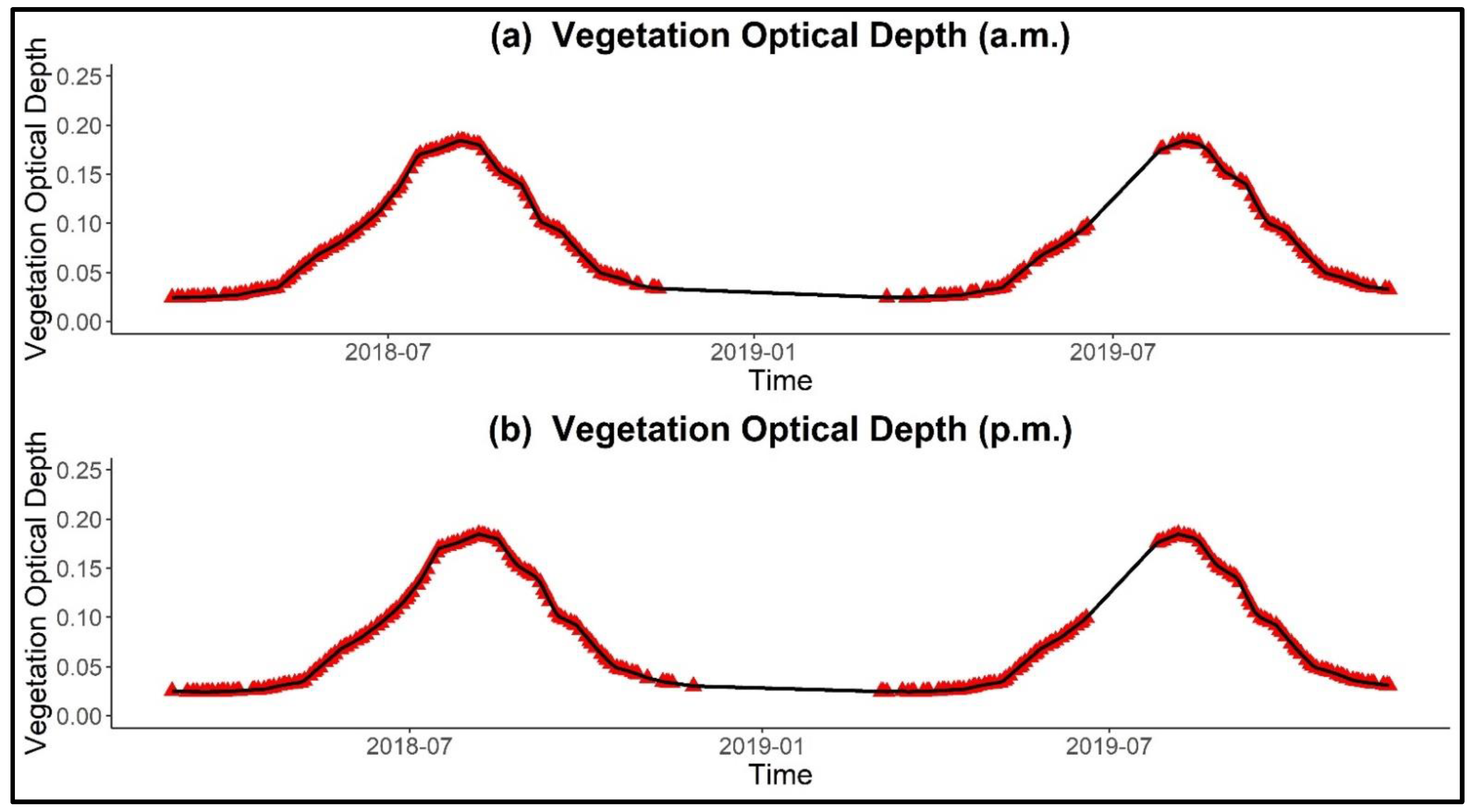
4.3. Impact of the Vegetation Optical Depth on the SMAP SM Retrieval Algorithm

The degree to which vegetation attenuates microwave radiation, known as the microwave vegetation optical depth (VOD), is proportional to the amount of water contained in the above-ground canopy biomass (known as the vegetation water content or VWC) [37,57,58], and thus represents a potentially useful indicator of the vegetation state. A layer of plants on top of the soil absorbs the soil’s emission and contributes its own emission to the overall radiative flux. A layer of vegetation over the soil attenuates the emission of the soil and adds to the total radiative flux with its own emission. The SMAP algorithms compute VOD from multi-year averaged MODIS (MOD13A2) NDVI datasets [59]. Potentially low soil emission might be caused by an increase in the NDVI, which indicates poor vegetation transmissivity. Soil emissivity decreases when SM increases.
Figure 14 shows the time-series variability of VOD obtained from SMAP L2 products at ascending and descending time steps. It is observed that there are high VOD values in the growing seasons (March to November) and low values in the non-growing season (December to February) during the study time period. Figure 6, Figure 7, and Figure 14 reveal that as the vegetation density increases, there is an increase in ubRMSE and a decrease in the correlation (R) value for SMAP L3 (a.m. and p.m.) SM products. A high VOD value causes an increase in vegetation attenuation and decreases the SM retrieval sensitivity of the SMAP algorithm. Table 2 shows that the SMAP SM estimation’s performance in the woodland is not good enough to be compared to the farmland and grassland, with a large ubRMSE and low correlation (R). The L4 products (surface and root-zone) show better results than the L3 products (a.m. and p.m.) for all types of vegetation covers. This shows that the VOD influences the SMAP L3 products’ algorithm more than the SMAP L4 products’ algorithm. Satellite-based SM assessment relies heavily on vegetation corrections for accurate SM retrieval [57].
The VOD values are directly linked to the vegetation type. Vegetation covers, such as forest and farmland, have a high canopy (high VOD) compared to grassland. High VOD values indicate lower transmittance of the plant layer and hence higher emissivity of the vegetation, which leads in a decrease in the soil emissivity, an increase in the soil dielectric constant, and eventually an increase in the SM values. Therefore, SMAP showed a better performance in the grassland where the vegetation cover did not cause uncertainty during SM estimation. Vegetation structure and VWC are major factors that affect the soil emissivity and vegetation transmissivity. High structure vegetation cover (woodland) contains a high amount of VWC due to its deeply distributed roots attenuating greater soil radiation [58]. Therefore, the SM retrievals contain more uncertainty in the woodland as compared to the farmland. In this sense, the hindrance of the vegetation cover in the grassland does not have much of an impact on SMAP SM estimation, showing better results (high correlation and less ubRMSE), as shown in Table 2. For the SMAP, it was found that a more precise estimation of SM can be obtained by employing the ancillary parameter VOD to compensate for the emissions attenuation induced by vegetation.

5. Conclusions

In this study, SMAP Level 3 (SPL3SMP_E) and Level 4 (SPL4SMGP) SM products were evaluated over the locations in the SM Network within the ShanDian River Basin during the period of 25 July 2018 to 31 December 2019 (according to the availability of in situ data). The following key findings were idenitified in this study:
(a)
The ubRMSE values for SPL4SMGP SSM and RZSM retrievals are less than 0.04 m 3 / m 3 for sparse network sites (M and L). The averaged ubRMSE of SPL4SMGP SSM (RZSM) estimates are about 0.037 m 3 / m 3 (0.017 m 3 / m 3 ) with correlation values of 0.62 (0.78) against the sparse network at a 9-km resolution, respectively. The core validation sites (S) showed ubRMSE values of 0.044 m 3 / m 3 (0.020 m 3 / m 3 ) for SSM (RZSM) estimates with the R values of 0.56 (0.48), respectively.
(b)
For SPL3SMP_E a.m. SM, the ubRMSE values are close to 0.04 m 3 / m 3 with R values larger than 0.56. The SPL3SMP_E a.m. (p.m.) SM has averaged ubRMSE values of 0.041 m 3 / m 3 (0.050 m 3 / m 3 ) with correlation values of 0.62 (0.42) against the sparse network at a 9-km resolution, respectively. The SPL3SMP_E p.m. SM estimates are less accurate than the a.m. retrievals.
(c)
For SSM evaluation, the skills of the SPL4SMGP SSM retrievals exceed that of the SPL3SMP_E (a.m. and p.m.) SM estimations.
(d)
Under different vegetation types, the SMAP L4 products performed well with high correlation (0.70) and less ubRMSE (0.019 m 3 / m 3 ) values than L3 products. Both products (L3 and L4) showed good accuracy in grassland, then farmland, and lowest in the woodland. The performance of these products was influenced by factors, such as the vegetation copy and physical surface temperature, in different study area locations.
The validation findings reported here can contribute to understanding the capability of SMAP SM products to express regional SM variations over various environmental situations. In addition, this study may contribute to the assessment of remote sensing SM assimilation studies by evaluating the uncertainties in SMAP SM products.

Author Contributions

Conceptualization, Y.Z. and A.A.N.; methodology, A.A.N. and Y.Z.; software, A.A.N., S.A. and M.A.; validation, A.A.N., Y.Z. and Z.J.; formal analysis, A.A.N., S.A. and M.M.A.; investigation, A.A.N. and M.A.; resources, Y.Z. and L.S.; data curation, A.A.N., M.M.A. and Z.J.; writing—original draft preparation, A.A.N. and Y.Z.; writing—review and editing, A.A.N. and G.R.; visualization, A.A.N. and S.A.; supervision, L.S.; project administration, L.S. and Y.Z.; funding acquisition, L.S. and Y.Z. All authors have read and agreed to the published version of the manuscript.

Funding

The project is funded by Natural Science Foundation of China through grants No. 51779179, 51609173, and 51861125202.

Institutional Review Board Statement

Not applicable.

Informed Consent Statement

Not applicable.

Data Availability Statement

Not applicable.

Conflicts of Interest

The authors declare no conflict of interest.

References

  1. Brocca, L.; Ciabatta, L.; Massari, C.; Camici, S.; Tarpanelli, A. Soil moisture for hydrological applications: Open questions and new opportunities. Water 2017, 9, 140. [Google Scholar] [CrossRef]
  2. Corradini, C. Soil moisture in the development of hydrological processes and its determination at different spatial scales. J. Hydrol. 2014, 516, 1–5. [Google Scholar] [CrossRef]
  3. De Rosnay, P.; Drusch, M.; Boone, A.; Balsamo, G.; Decharme, B.; Harris, P.; Kerr, Y.; Pellarin, T.; Polcher, J.; Wigneron, J.P. AMMA land surface model intercomparison experiment coupled to the community microwave emission model: ALMIP-MEM. J. Geophys. Res. Atmos. 2009, 114, D05108. [Google Scholar] [CrossRef]
  4. Miralles, D.G.; Van Den Berg, M.J.; Gash, J.H.; Parinussa, R.M.; De Jeu, R.A.M.; Beck, H.E.; Holmes, T.R.H.; Jiménez, C.; Verhoest, N.E.C.; Dorigo, W.A.; et al. El Niño-La Niña cycle and recent trends in continental evaporation. Nat. Clim. Chang. 2014, 4, 122–126. [Google Scholar] [CrossRef]
  5. Hirschi, M.; Seneviratne, S.I.; Alexandrov, V.; Boberg, F.; Boroneant, C.; Christensen, O.B.; Formayer, H.; Orlowsky, B.; Stepanek, P. Observational evidence for soil-moisture impact on hot extremes in southeastern Europe. Nat. Geosci. 2011, 4, 17–21. [Google Scholar] [CrossRef]
  6. Massari, C.; Brocca, L.; Moramarco, T.; Tramblay, Y.; Didon Lescot, J.F. Potential of soil moisture observations in flood modelling: Estimating initial conditions and correcting rainfall. Adv. Water Resour. 2014, 74, 44–53. [Google Scholar] [CrossRef]
  7. Dorigo, W.A.; Xaver, A.; Vreugdenhil, M.; Gruber, A.; Hegyiová, A.; Sanchis-Dufau, A.D.; Zamojski, D.; Cordes, C.; Wagner, W.; Drusch, M. Global Automated Quality Control of In Situ Soil Moisture Data from the International Soil Moisture Network. Vadose Zone J. 2013, 12, vzj2012.0097. [Google Scholar] [CrossRef]
  8. An, R.; Zhang, L.; Wang, Z.; Quaye-Ballard, J.A.; You, J.; Shen, X.; Gao, W.; Huang, L.J.; Zhao, Y.; Ke, Z. Validation of the ESA CCI soil moisture product in China. Int. J. Appl. Earth Obs. Geoinf. 2016, 48, 28–36. [Google Scholar] [CrossRef]
  9. Entekhabi, D.; Njoku, E.G.; O’Neill, P.E.; Kellogg, K.H.; Crow, W.T.; Edelstein, W.N.; Entin, J.K.; Goodman, S.D.; Jackson, T.J.; Johnson, J.; et al. The soil moisture active passive (SMAP) mission. Proc. IEEE 2010, 98, 704–716. [Google Scholar] [CrossRef]
  10. Piepmeier, J.R.; Focardi, P.; Horgan, K.A.; Knuble, J.; Ehsan, N.; Lucey, J.; Brambora, C.; Brown, P.R.; Hoffman, P.J.; French, R.T.; et al. SMAP L-Band Microwave Radiometer: Instrument Design and First Year on Orbit. IEEE Trans. Geosci. Remote Sens. 2017, 55, 1954–1966. [Google Scholar] [CrossRef] [Green Version]
  11. Kerr, Y.H.; Njoku, E.G. A Semiempirical Model for Interpreting Microwave Emission from Semiarid Land Surfaces as Seen from Space. IEEE Trans. Geosci. Remote Sens. 1990, 28, 384–393. [Google Scholar] [CrossRef]
  12. Hoang, K.O.; Lu, M. Assessment of the temperature effects in smap satellite soil moisture products in oklahoma. Remote Sens. 2021, 13, 4104. [Google Scholar] [CrossRef]
  13. Xu, X. Evaluation of smap level 2, 3, and 4 soil moisture datasets over the Great Lakes region. Remote Sens. 2020, 12, 3785. [Google Scholar] [CrossRef]
  14. Cui, C.; Xu, J.; Zeng, J.; Chen, K.S.; Bai, X.; Lu, H.; Chen, Q.; Zhao, T. Soil moisture mapping from satellites: An intercomparison of SMAP, SMOS, FY3B, AMSR2, and ESA CCI over two dense network regions at different spatial scales. Remote Sens. 2018, 10, 33. [Google Scholar] [CrossRef] [Green Version]
  15. Ducharne, A.; Koster, R.D.; Suarez, M.J.; Stieglitz, M.; Kumar, P. A catchment-based approach to modeling land surface processes in a general circulation model 2. Parameter estimation and model demonstration. J. Geophys. Res. Atmos. 2000, 105, 24823–24838. [Google Scholar] [CrossRef]
  16. Koster, R.D.; Suarez, M.J.; Ducharne, A.; Stieglitz, M.; Kumar, P. A catchment-based approach to modeling land surface processes in a general circulation model: 1. Model structure. J. Geophys. Res. Atmos. 2000, 105, 24809–24822. [Google Scholar] [CrossRef]
  17. De Lannoy, G.J.M.; Reichle, R.H. Assimilation of SMOS brightness temperatures or soil moisture retrievals into a land surface model. Hydrol. Earth Syst. Sci. 2016, 20, 4895–4911. [Google Scholar] [CrossRef] [Green Version]
  18. De Lannoy, G.J.M.; Reichle, R.H. Global assimilation of multiangle and multipolarization SMOS brightness temperature observations into the GEOS-5 catchment land surface model for soil moisture estimation. J. Hydrometeorol. 2016, 17, 669–691. [Google Scholar] [CrossRef] [Green Version]
  19. Su, Z.; Wen, J.; Dente, L.; Van Der Velde, R.; Wang, L.; Ma, Y.; Yang, K.; Hu, Z. The tibetan plateau observatory of plateau scale soil moisture and soil temperature (Tibet-Obs) for quantifying uncertainties in coarse resolution satellite and model products. Hydrol. Earth Syst. Sci. 2011, 15, 2303–2316. [Google Scholar] [CrossRef] [Green Version]
  20. Su, Z.; De Rosnay, P.; Wen, J.; Wang, L.; Zeng, Y. Evaluation of ECMWF’s soil moisture analyses using observations on the Tibetan Plateau. J. Geophys. Res. Atmos. 2013, 118, 5304–5318. [Google Scholar] [CrossRef] [Green Version]
  21. Chen, Y.; Yang, K.; Qin, J.; Zhao, L.; Tang, W.; Han, M. Evaluation of AMSR-E retrievals and GLDAS simulations against observations of a soil moisture network on the central Tibetan Plateau. J. Geophys. Res. Atmos. 2013, 118, 4466–4475. [Google Scholar] [CrossRef]
  22. Liu, Q.; Du, J.Y.; Shi, J.C.; Jiang, L.M. Analysis of spatial distribution and multi-year trend of the remotely sensed soil moisture on the Tibetan Plateau. Sci. China Earth Sci. 2013, 56, 2173–2185. [Google Scholar] [CrossRef]
  23. Bi, H.; Ma, J.; Zheng, W.; Zeng, J. Comparison of soil moisture in GLDAS model simulations and in situ observations over the Tibetan Plateau. J. Geophys. Res. 2016, 121, 2658–2678. [Google Scholar] [CrossRef] [Green Version]
  24. Ma, C.; Li, X.; Wei, L.; Wang, W. Multi-scale validation of SMAP soil moisture products over cold and arid regions in Northwestern China using distributed ground observation data. Remote Sens. 2017, 9, 327. [Google Scholar] [CrossRef] [Green Version]
  25. Zhang, X.; Zhang, T.; Zhou, P.; Shao, Y.; Gao, S. Validation analysis of SMAP and AMSR2 soil moisture products over the United States using ground-based measurements. Remote Sens. 2017, 9, 104. [Google Scholar] [CrossRef] [Green Version]
  26. Li, C.; Lu, H.; Yang, K.; Han, M.; Wright, J.S.; Chen, Y.; Yu, L.; Xu, S.; Huang, X.; Gong, W. The evaluation of SMAP enhanced soil moisture products using high-resolution model simulations and in-situ observations on the Tibetan Plateau. Remote Sens. 2018, 10, 535. [Google Scholar] [CrossRef] [Green Version]
  27. Hu, F.; Wei, Z.; Zhang, W.; Dorjee, D.; Meng, L. A spatial downscaling method for SMAP soil moisture through visible and shortwave-infrared remote sensing data. J. Hydrol. 2020, 590, 125360. [Google Scholar] [CrossRef]
  28. Colliander, A.; Reichle, R.; Crow, W.; Cosh, M.; Chen, F.; Chan, S.; Das, N.; Bindlish, R.; Chaubell, J.; Kim, S.; et al. Validation of Soil Moisture Data Products from the NASA SMAP Mission. IEEE J. Sel. Top. Appl. Earth Obs. Remote Sens. 2021, 15, 364–392. [Google Scholar] [CrossRef]
  29. Al-Yaari, A.; Wigneron, J.P.; Dorigo, W.; Colliander, A.; Pellarin, T.; Hahn, S.; Mialon, A.; Richaume, P.; Fernandez-Moran, R.; Fan, L.; et al. Assessment and inter-comparison of recently developed/reprocessed microwave satellite soil moisture products using ISMN ground-based measurements. Remote Sens. Environ. 2019, 224, 289–303. [Google Scholar] [CrossRef]
  30. O’Neill, P.E.; Chan, S.; Njoku, E.G.; Jackson, T.; Bindlish, R.; Chaubell, J. SMAP Enhanced L3 Radiometer Global Daily 9 km EASE-Grid Soil Moisture, Version 4; National Snow and Ice Data Center: Boulder, CO, USA, 2020; pp. 1–26. [Google Scholar]
  31. Fascetti, F.; Pierdicca, N.; Pulvirenti, L.; Crapolicchio, R. SMOS, ASCAT, SMAP and ERA soil moisture comparison through the triple and quadruple collocation technique. In Proceedings of the SPIE Remote Sensing, Edinburgh, UK, 26–29 September 2016; Volume 10003, p. 100030H. [Google Scholar] [CrossRef]
  32. Reichle, R.H.; de Lannoy, G.J.M.; Liu, Q.; Koster, R.D.; Kimball, J.S.; Crow, W.T.; Ardizzone, J.V.; Chakraborty, P.; Collins, D.W.; Conaty, A.L.; et al. Global assessment of the SMAP Level-4 surface and root-zone soil moisture product using assimilation diagnostics. J. Hydrometeorol. 2017, 18, 3217–3237. [Google Scholar] [CrossRef]
  33. Chen, F.; Crow, W.T.; Bindlish, R.; Colliander, A.; Burgin, M.S.; Asanuma, J.; Aida, K. Global-scale evaluation of SMAP, SMOS and ASCAT soil moisture products using triple collocation. Remote Sens. Environ. 2018, 214, 1–13. [Google Scholar] [CrossRef] [PubMed]
  34. Burgin, M.S.; Colliander, A.; Njoku, E.G.; Chan, S.K.; Cabot, F.; Kerr, Y.H.; Bindlish, R.; Jackson, T.J.; Entekhabi, D.; Yueh, S.H. A Comparative Study of the SMAP Passive Soil Moisture Product with Existing Satellite-Based Soil Moisture Products. IEEE Trans. Geosci. Remote Sens. 2017, 55, 2959–2971. [Google Scholar] [CrossRef] [PubMed]
  35. Colliander, A.; Cosh, M.H.; Misra, S.; Jackson, T.J.; Crow, W.T.; Chan, S.; Bindlish, R.; Chae, C.; Holifield Collins, C.; Yueh, S.H. Validation and scaling of soil moisture in a semi-arid environment: SMAP validation experiment 2015 (SMAPVEX15). Remote Sens. Environ. 2017, 196, 101–112. [Google Scholar] [CrossRef]
  36. Colliander, A.; Cosh, M.H.; Misra, S.; Jackson, T.J.; Crow, W.T.; Powers, J.; McNairn, H.; Bullock, P.; Berg, A.; Magagi, R.; et al. Comparison of high-resolution airborne soil moisture retrievals to SMAP soil moisture during the SMAP validation experiment 2016 (SMAPVEX16). Remote Sens. Environ. 2019, 227, 137–150. [Google Scholar] [CrossRef]
  37. Jackson, T.J.; Schmugge, T.J. Vegetation effects on the microwave emission of soils. Remote Sens. Environ. 1991, 36, 203–212. [Google Scholar] [CrossRef]
  38. Njoku, E.G.; Entekhabi, D. Passive microwave remote sensing of soil moisture. J. Hydrol. 1996, 184, 101–129. [Google Scholar] [CrossRef]
  39. Wraith, J.M.; Or, D. Temperature effects on soil bulk dielectric permittivity measured by time domain reflectometry: Experimental evidence and hypothesis development. Water Resour. Res. 1999, 35, 361–369. [Google Scholar] [CrossRef]
  40. Zhao, T.; Shi, J.; Lv, L.; Xu, H.; Chen, D.; Cui, Q.; Jackson, T.J.; Yan, G.; Jia, L.; Chen, L.; et al. Soil moisture experiment in the Luan River supporting new satellite mission opportunities. Remote Sens. Environ. 2020, 240, 111680. [Google Scholar] [CrossRef]
  41. Cui, H.; Jiang, L.; Du, J.; Zhao, S.; Wang, G.; Lu, Z.; Wang, J. Evaluation and analysis of AMSR-2, SMOS, and SMAP soil moisture products in the Genhe area of China. J. Geophys. Res. Atmos. 2017, 122, 8650–8666. [Google Scholar] [CrossRef]
  42. Kellogg, K.; Thurman, S.; Edelstein, W.; Spencer, M.; Chen, G.S.; Underwood, M.; Njoku, E.; Goodman, S.; Jai, B. NASA’s soil moisture active passive (SMAP) observatory. In Proceedings of the 2013 IEEE Aerospace Conference, Big Sky, MT, USA, 2–9 March 2013; pp. 1–20. [Google Scholar] [CrossRef]
  43. Entekhabi, D.; Yueh, S.; O’Neil, P.E.; Kellogg, K.H.; Allen, A.; Bindlish, R.; Brown, M.; Chan, S.; Colliander, A.; Crow, W.T.; et al. SMAP Handbook: Soil Moisture Active Passive, Mapping Soil Moisture and Freeze/Thaw from Space; National Aeronautics and Space Administration: Washington, DC, USA, 2014; p. 192.
  44. Reichle, R.; De Lannoy, G.; Koster, R.D.; Crow, W.T.; Kimball, J.S.; Liu, Q. SMAP L4 Global 3-Hourly 9 km EASE-Grid Surface and Root Zone Soil Moisture Analysis Update, Version 4; National Snow and Ice Data Center: Boulder, CO, USA, 2018. [Google Scholar]
  45. Chan, S.K.; Bindlish, R.; O’Neill, P.; Jackson, T.; Njoku, E.; Dunbar, S.; Chaubell, J.; Piepmeier, J.; Yueh, S.; Entekhabi, D.; et al. Development and assessment of the SMAP enhanced passive soil moisture product. Remote Sens. Environ. 2018, 204, 931–941. [Google Scholar] [CrossRef] [Green Version]
  46. Qiu, J.; Dong, J.; Crow, W.T.; Zhang, X.; Reichle, R.H.; De Lannoy, G.J.M. The benefit of brightness temperature assimilation for the SMAP Level-4 surface and root-zone soil moisture analysis. Hydrol. Earth Syst. Sci. 2021, 25, 1569–1586. [Google Scholar] [CrossRef]
  47. Rodriguez-Iturbe, I.; Vogel, G.K.; Rigon, R.; Entekhabi, D.; Castelli, F.; Rinaldo, A. On the spatial organization of soil moisture fields. Geophys. Res. Lett. 1995, 22, 2757–2760. [Google Scholar] [CrossRef]
  48. Entekhabi, D.; Reichle, R.H.; Koster, R.D.; Crow, W.T. Performance metrics for soil moisture retrievals and application requirements. J. Hydrometeorol. 2010, 11, 832–840. [Google Scholar] [CrossRef]
  49. Reichle, R.H.; Koster, R.D.; Liu, P.; Mahanama, S.P.P.; Njoku, E.G.; Owe, M. Comparison and assimilation of global soil moisture retrievals from the Advanced Microwave Scanning Radiometer for the Earth Observing System (AMSR-E) and the Scanning Multichannel Microwave Radiometer (SMMR). J. Geophys. Res. Atmos. 2007, 112, D09108. [Google Scholar] [CrossRef]
  50. Zhang, L.; He, C.; Zhang, M. Multi-scale evaluation of the SMAP product using sparse in-situ network over a high mountainous Watershed, Northwest China. Remote Sens. 2017, 9, 1111. [Google Scholar] [CrossRef] [Green Version]
  51. Derksen, C.; Xu, X.; Scott Dunbar, R.; Colliander, A.; Kim, Y.; Kimball, J.S.; Black, T.A.; Euskirchen, E.; Langlois, A.; Loranty, M.M.; et al. Retrieving landscape freeze/thaw state from Soil Moisture Active Passive (SMAP) radar and radiometer measurements. Remote Sens. Environ. 2017, 194, 48–62. [Google Scholar] [CrossRef]
  52. Reichle, R.H.; De Lannoy, G.J.M.; Liu, Q.; Ardizzone, J.V.; Colliander, A.; Conaty, A.; Crow, W.; Jackson, T.J.; Jones, L.A.; Kimball, J.S.; et al. Assessment of the SMAP Level-4 surface and root-zone soil moisture product using in situ measurements. J. Hydrometeorol. 2017, 18, 2621–2645. [Google Scholar] [CrossRef]
  53. Wang, Z.; Che, T.; Zhao, T.; Dai, L.; Li, X.; Wigneron, J.P. Evaluation of SMAP, SMOS, and AMSR2 soil moisture products based on distributed ground observation network in cold and arid regions of China. IEEE J. Sel. Top. Appl. Earth Obs. Remote Sens. 2021, 14, 8955–8970. [Google Scholar] [CrossRef]
  54. Jackson, T.J.; Cosh, M.H.; Bindlish, R.; Starks, P.J.; Bosch, D.D.; Seyfried, M.; Goodrich, D.C.; Moran, M.S.; Du, J. Validation of advanced microwave scanning radiometer soil moisture products. IEEE Trans. Geosci. Remote Sens. 2010, 48, 4256–4272. [Google Scholar] [CrossRef]
  55. Thomas, J.J. Measuring Surface Soil Moisture Using Passive Microwave Remote Sensing. Hydrol. Process. 1993, 7, 139–152. [Google Scholar]
  56. Leroux, D.J.; Kerr, Y.H.; Al Bitar, A.; Bindlish, R.; Jackson, T.J.; Berthelot, B.; Portet, G. Comparison between SMOS, VUA, ASCAT, and ECMWF soil moisture products over four watersheds in U.S. IEEE Trans. Geosci. Remote Sens. 2014, 52, 1562–1571. [Google Scholar] [CrossRef] [Green Version]
  57. Konings, A.G.; Piles, M.; Das, N.; Entekhabi, D. L-band vegetation optical depth and effective scattering albedo estimation from SMAP. Remote Sens. Environ. 2017, 198, 460–470. [Google Scholar] [CrossRef]
  58. Tian, F.; Wigneron, J.P.; Ciais, P.; Chave, J.; Ogée, J.; Peñuelas, J.; Ræbild, A.; Domec, J.C.; Tong, X.; Brandt, M.; et al. Coupling of ecosystem-scale plant water storage and leaf phenology observed by satellite. Nat. Ecol. Evol. 2018, 2, 1428–1435. [Google Scholar] [CrossRef] [PubMed] [Green Version]
  59. Podest, E.; Crow, W.T. SMAP Ancillary Data Report on Digital Elevation Model, Jet Propulsion Laboratory Ancillary Data Report; California Institute of Technology: Pasadena, CA, USA, 2013. [Google Scholar]
Figure 1. The ShanDian River Basin and the Network within the ShanDian River Basin (SMN-SDR), (a) land use map of the study area, (b) providing in situ SM measurements at a small scale (red circles within the red rectangles), medium scale (blue triangles within the blue rectangles), and large scale (green squares within the rectangles).
Remotesensing 14 00982 g001
Figure 2. Time series evaluation of SPL4SMGP SSM and station averaged in situ SM at different spatial locations, (a) S-scale stations, (b) M-scale stations, (c) L-scale stations.
Remotesensing 14 00982 g002
Figure 3. Time series evaluation of SPL4SMGP RZSM and station averaged in situ SM at different spatial locations, (a) S-scale stations, (b) M-scale stations, (c) L-scale stations.
Remotesensing 14 00982 g003
Figure 4. Performance metrics (R (a,d), ubRMSE (b,e), bias (c,f)) for SPL4SMGP SSM (top row) and RZSM (bottom row) retrievals at S-scale, M-scale, and L-scale stations.
Remotesensing 14 00982 g004
Figure 5. The averaged performance metrics (R (a), ubRMSE (b), and bias (c)) for the SPL4SMGP SSM and RZSM estimations against the sparse network sites (across 34 validation sites).
Remotesensing 14 00982 g005
Figure 6. Comparison of SPL3SMP E (a.m.) SM and station averaged in situ data (hourly composite of SSM) at different spatial locations, (a) S-scale stations, (b) M-scale stations, (c) L-scale stations.
Remotesensing 14 00982 g006
Figure 7. Comparison of SPL3SMP E (p.m.) SM and station averaged in situ data (hourly composite of SSM) at different spatial locations, (a) S-scale stations, (b) M-scale stations, (c) L-scale stations.
Remotesensing 14 00982 g007
Figure 8. Performance metrics (R (a,d), ubRMSE (b,e), bias (d,f)) for SPL3SMP_E a.m. (top row) and (bottom row) p.m. SM estimates at S-scale, M-scale, and L-scale sites.
Remotesensing 14 00982 g008
Figure 9. The averaged performance metrics (R (a), ubRMSE (b), and bias (c)) for the SPL3SMP_E a.m. and p.m. SM estimates against the sparse network sites (across 34 validation sites).
Remotesensing 14 00982 g009
Figure 10. Comparison of SPL3SMP_E (a.m.), SPL3SMP_E (p.m.) and SPL4SMGP SSM and station averaged in situ data (hourly composite of SSM) at different spatial locations, (a) S-scale stations, (b) M-scale stations, (c) L-scale stations.
Remotesensing 14 00982 g010
Figure 11. Comparison of evaluation metrics (R (a,d,g), ubRMSE (b,e,h), and bias (c,f,i)) for SPL3SMP_E (a.m. and p.m.) and SPL4SMGP SSM estimates for S-scale, M-scale, and L-scale sites.
Remotesensing 14 00982 g011
Figure 12. Scatter plots between estimated SM from SMAP products (SPL3SMP_E and SPL4SMGP) and in situ data observed from SMN-SDR for (a) S-scale, (b) M-scale, (c) L-scale.
Remotesensing 14 00982 g012
Figure 13. Time-series of averaged in situ T and SMAP T for the (a) a.m. and (b) p.m. orbits in the assessment domain.
Remotesensing 14 00982 g013
Figure 14. Time-series representation of SMAP-derived vegetation optical depth (dimensionless) of (a) SMAP L3 (a.m.) products and (b) SMAP L3 (p.m.) products.
Remotesensing 14 00982 g014
Table 1. Specifications of in situ soil moisture stations at the SMN-SDR.
Station IDLongitude
(Degree)
Latitude
(Degree)
Setup Time
(Local Time)
Elevation
(m)
Vegetation Cover
S1115.94571742.00663919 July 2018 12:531368Farmland
S2115.93780042.04017219 July 2018 15:001363Grassland
S3115.91940042.05714418 July 2018 18:401343Grassland
S4115.93506942.0826694 September 2018 10:171357Grassland
S5115.89405042.07393918 July 2018 15:301327Grassland
S6115.86573342.04554428 September 2018 11:041331Grassland
S7115.89611142.02972214 August 2018 09:081332Grassland
S8115.87305642.0175004 August 2018 18:361334Grassland
M1115.85592841.9655724 September 2018 11:561343Grassland
M2115.80944442.10527814 August 2018 11:301451Grassland
M3116.08250041.94972214 August 2018 15:411466Farmland
M4116.18550842.09595621 July 2018 09:511394Grassland
M5116.18823642.18555320 July 2018 14:301433Grassland
M6115.93874242.1868004 September 2018 09:021308Grassland
M7115.96818142.17698318 July 2018 12:301330Grassland
M8115.88861142.30638913 August 2018 10:501363Grassland
M9116.07037242.30553913 August 2018 14:131280Grassland
M10116.24275342.30256713 August 2018 17:221327Woodland
M11116.13948342.16893320 July 2018 16:351470Grassland
M12116.17660342.02509721 July 2018 08:181354Grassland
L1115.53885341.5507611 September 2018 11:121433Grassland
L2115.60314241.7800691 September 2018 13:401401Grassland
L3115.62838342.0421751 September 2018 17:301452Grassland
L4115.68970842.2576112 September 2018 11:541338Grassland
L5115.74280842.4197422 September 2018 09:491427Grassland
L6116.33330341.8029475 September 2018 14:271369Grassland
L7116.34237842.2140893 September 2018 13:511364Woodland
L8116.36103141.9553113 September 2018 11:151435Grassland
L9116.08734241.7447364 September 2018 15:421443Grassland
L10115.94507841.7469114 September 2018 13:531410Grassland
L11116.22271142.4119722 September 2018 14:191280Grassland
L12116.36777542.4012062 September 2018 16:071315Grassland
L13115.99655842.4164313 September 2018 17:241329Grassland
L14116.43741441.5744335 September 2018 11:191383Grassland
Table 2. Comparison of the SMAP SM L3 and L4 products in the SMN-SDR Basin under different vegetation covers.
The L3 a.m. ProductThe L3 p.m. Product
Vegetation
Types
RRMSE
( m 3 / m 3 )
Bias
( m 3 / m 3 )
ubRMSE
( m 3 / m 3 )
NRRMSE
( m 3 / m 3 )
Bias ( m 3 / m 3 ) ubRMSE
( m 3 / m 3 )
N
Grassland0.2550.090-0.0710.0561460.4810.076−0.0600.047160
Farmland0.4320.068-0.0430.0521460.3310.067−0.0350.057160
Woodland0.2750.059-0.0130.0591460.0840.065−0.0010.065160
The L4 SSM ProductThe L4 RZSM Product
Vegetation
Types
RRMSE
( m 3 / m 3 )
Bias
( m 3 / m 3 )
ubRMSE
( m 3 / m 3 )
NRRMSE
( m 3 / m 3 )
Bias
( m 3 / m 3 )
ubRMSE
( m 3 / m 3 )
N
Grassland0.4470.051−0.0240.04525040.7070.0400.0360.0192504
Farmland0.3850.0520.0010.05224960.2690.0520.0410.0312496
Woodland0.2030.0650.0430.04222960.6330.1060.1060.0332296
Publisher’s Note: MDPI stays neutral with regard to jurisdictional claims in published maps and institutional affiliations.

