The Suitability of PlanetScope Imagery for Mapping Rubber Plantations

Abstract

Quickly and accurately understanding the spatial distribution of regional rubber resources is of great practical significance. Using the unique phenological characteristics of rubber trees derived from remotely sensed data is a common effective method for monitoring rubber trees. However, due to the lack of high-quality images available during the key phenological period, it is still very difficult to apply this method in practical applications. PlanetScope data with high temporal (daily) resolution have great advantages in acquiring high-quality images, but these images have not been previously used to monitor rubber plantations. In this paper, multitemporal PlanetScope images were used as data sources, and the spectral features, index features, first principal components, and textural features of the images were comprehensively utilized. Four classification methods, including a pixel-based random forest (RF) approach, pixel-based support vector machine (SVM) approach, object-oriented RF approach and object-oriented SVM approach, were utilized to discuss the feasibility of using PlanetScope data to monitor rubber forests. The results showed that the optimal time window for monitoring rubber forests in the study area spanned from the 49th day to the 65th day of 2019 according to the MODIS-NDVI analysis. The contribution rate of the difference in the modified simple ratio (dMSR) feature was largest among all considered features for all pixel-based and object-oriented methods. The object-oriented RF/SVM classification method achieved the best classification results with an overall accuracy of 93.87% and a Kappa index of agreement (KIA) of 0.92. The highest producer’s accuracy and user’s accuracy obtained with this method were 95.18% for rubber plantations. The results of this study show that it is feasible to use PlanetScope data to perform rubber monitoring, thus effectively solving the problem of missing images in the optimal rubber monitoring period; additionally, this method can be extended to other real-life applications.

1. Introduction

Rubber trees (Hevea brasiliensis) are important sources of natural rubber and wood products that meet commodity production requirements. Rubber tree development in the region of study is often affected by local government policies and the potential economic benefits. It is crucial to conduct accurate and up-to-date monitoring and mapping of the rubber plantation distribution to ensure the health of the rubber industry in the region of study. Compared with traditional manual survey methods, remote sensing technologies have the ability to survey large study areas and rapidly acquire ground object information; these technologies have been widely used in various agricultural fields. However, the monitoring of rubber forests based on remote sensing technology is recently new, and extensive research is lacking. The first report about rubber mapping with remote sensing was published in 2002 [1], and only a total of 24 documents focusing on this field were published through December 2020 based on searches [2] of six bibliographical databases (Science Direct, Web of Science Core Collection, Scopus, ProQuest and Google Scholar) with the keywords “remote sensing” and “rubber plantation”. These studies can be summarized as follows.

In terms of the remote sensing data used, according to the spatial resolution, the remote sensing images considered in the existing studies can be classified into four classes: low resolution (MODIS [3]), moderate resolution (Landsat [1,4,5,6,7,8,9,10,11,12,13,14,15,16,17,18], PALSAR [19], ASTER [20], IRS [21,22], THEOS [23]), high resolution (Sentinel-2 [17,24], GaoFen-1 [17]), and very high resolution (IKONOS [25]). Single-date image information was primarily considered when mapping rubber plantations in early studies. Considering the unique wintertime phenological characteristics of rubber, such as defoliation and refoliation, multitemporal remote sensing images were adopted to obtain temporally variable features to use in estimates [3,6,7,8,9,10,11,12,13,14,15,16,19,24]. It was verified that the method based on multiple phenology information can improve rubber estimation results [9,10]. Landsat TM/ETM+ is currently the most broadly used sensor in rubber plantation estimation studies, especially multitemporal analyses, due to the advantages associated with its high revisit time of 16 days [2]. However, the cloudy climate conditions in the tropics introduce challenges for optical sensors; therefore, it has been very difficult to popularize this method for studies of specific periods and over large regions [9,10].

In terms of the estimation approaches used, supervised classifiers, including maximum likelihood [26], the Mahalanobis typicalities [3,18], the Mahalanobis typicalities with a neural network [20], decision tree [7,11,13,14,15,16,18,24,25], K-nearest neighbor [11,18,27], support vector machine [18,28], and random forest [17] classifiers, are commonly used to map rubber plantations based on remote sensing. Most previous studies used pixel information to estimate rubber plantation characteristics, and only three papers [11,18,27] have discussed the use of the object-oriented classification approach for monitoring rubber plantations. In these papers, spectral information was mostly considered; other features, such as textural features, have rarely been discussed. In addition, among these studies, the same supervised classifier used can provide different classification results because of different remote sensing images, features, methods, and study regions. For example, Zhai et al. [11], Dibs et al. [18], and Xiao et al. [24] used a decision tree classifier to map rubber plantations and obtained the classification accuracies of 77.5%, 80.80%, and 92.50%, respectively. The performances of these methods proposed in different studies cannot be comparatively evaluated directly. Thus, rubber mapping based on remote sensing still lacks systematic and comprehensive research with different remote sensing images, such as PlanetScope data, different approaches, such as object-based method and pixel-based method, and different features, such as texture features and spectral features, have not been fully considered.

PlanetScope images were acquired by PlanetInc. in America, the world’s largest satellite constellation, with more than 170 orbiting satellites. PlanetScope data have high spatial (3–4 m) and temporal (daily) resolutions, which has been successfully applied on many fields, for example, crop yield estimation [29], crop leaf area index estimation [30], pasture biomass [31], tropical forest canopy height [32] and so on. Csillik et al. [32] used the high temporal resolutions of Planet images, in view of limited capabilities of frequent updating of moderate resolution satellite data, to estimate top-of-canopy height of tropical forests. It has a significant advantage in acquiring high-quality images during the critical monitoring window period of rubber, which is very important to map rubber plantations by remote sensing. However, these data have not been used to monitor rubber plantations up to now [2].

Therefore, in this paper, we use PlanetScope images and comprehensively utilize four features, namely, spectral, vegetation index, first principal component, and textural features, to build pixel-based RF/SVM and object-oriented RF/SVM approaches to conduct rubber-monitoring research. The objectives are to assess the feasibility of monitoring rubber forests with PlanetScope data and to propose a practical and feasible monitoring method.

2. Materials and Methods

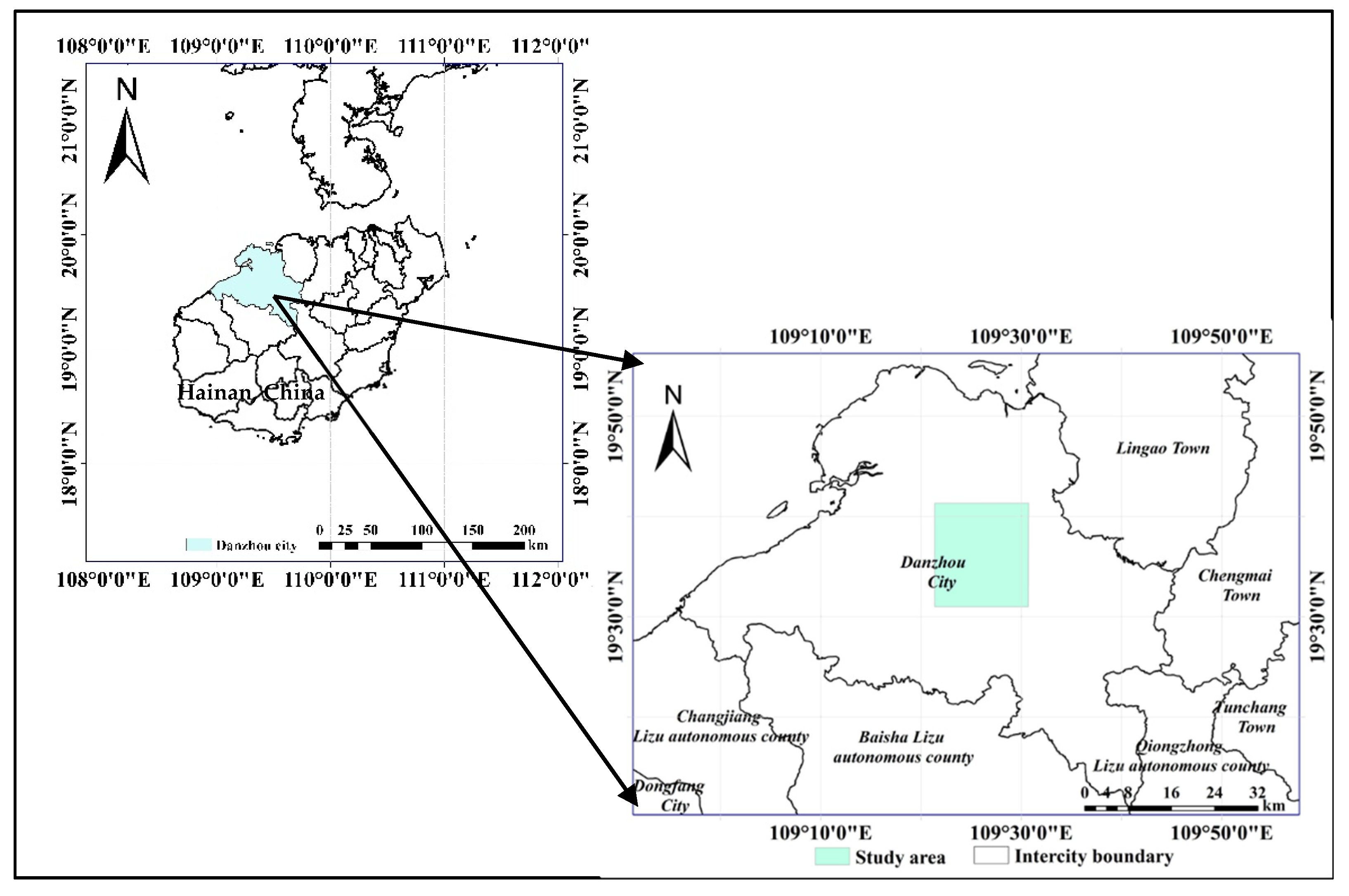
2.1. Study Area

Danzhou city is in northwestern Hainan Province, China, within coordinates ranging from 19°11′~19°52′N and from 108°56′~109°46′E. This city has the largest land area (3398 km²) and the longest coastline (307 km) of any city in Hainan Province. The region has a tropical monsoon marine climate, with an average annual temperature of 23.1 °C and an average annual rainfall total of 1823 mm. The terrain is mainly hilly, and from southeast to northwest, the ground surface gradually inclines downwards; the elevations are high in the southeast and low in the northwest, and the south and southeast regions contain low, hilly areas. As one of the major rubber plantation areas in China, the rubber plantation area in Danzhou city was 848.20 km² in 2019, and the total yield was 60,969,000 kg according to statistics [33] (p. 286). With the development of rubber plantations in China over the past 100 years, Danzhou city has developed into one of the dominant regions in terms of its rubber plantation area, rubber latex quantity and yield among all rubber plantation regions in China. The research region considered in our study is located in eastern Danzhou city and includes Xiqing Farm and some regions of Dongcheng town, Nada town, Dacheng town, and other areas (see Figure 1). Rubber trees display obvious phenological change characteristics. According to the growth changes of rubber buds and leaves, the phenological stages can be divided into the red leaf stage, deciduous stage, fresh leaf stage (sprout stage, elongating stage, bronze stage, color-changing stage, light green stage, and stable stage) and mature leaf stage within a year, and these cyclic changes are shown in Figure 2. The workflow by which rubber plantations were mapped in this study is shown in Figure 3.

2.2. Data

2.2.1. MODIS Data

Since rubber trees cycle through mature leaf, red leaf, defoliation and fresh leaf periods (Figure 2), the lowest NDVI value can be found according to the MODIS-NDVI time series curve to determine the specific times of defoliation and leaf extraction in rubber forests. This method has been verified by Liao et al. [8] and Liu et al. [7]. The MODIS data in this study were MOD13Q1-NDVI products obtained from January to December 2019 with a 16-day return period and a 250-m spatial resolution; these products are typically used to study land surface and vegetation conditions. The MODIS images taken in Hainan Province were denoted H28V07, and a total of 23 images were collected in 2019. These data were downloaded from the Level-1 and Atmosphere Archive & Distribution System Distributed Active Archive Center Website (https://ladsweb.modaps.eosdis.nasa.gov, accessed on 14 August 2019). The NDVI time series for 23 rubber forests in the study area were acquired to provide a basis for determining the optimal remote sensing monitoring time.

2.2.2. PlanetScope Imagery Data

PlanetScope images were acquired by Planet Inc., the world’s largest satellite constellation, with more than 170 orbiting satellites; together, this constellation can monitor the whole world once per day. PlanetScope satellites are the world’s only remote sensing satellites with high-resolution, high-frequency, and full coverage capabilities globally. In the study, we selected PlanetScope images that were acquired on the 27th of February and the 8th of June, 2019, and were clear and cloud free. The spatial resolution of the satellite images was 3 m, and each image included four spectral bands: the blue, green, red and near-infrared bands. The PlanetScope images used in this study were ortho-grade (3B) data products; these imageries have undergone a series of processes (including sensor correction, radiation correction, atmospheric correction, and geometric correction) to obtain true and reliable surface reflectance images. The main parameters of the PlanetScope satellites are shown in

Table 1. Main parameters of the PlanetScope satellites.

Parameter	Value	Parameter	Value
Orbit	International Space Station’s orbit Sun-synchronous orbit	Orbit Altitude	400 km 475 km
Orbit inclination	52° 98°	Sensor type	Bayer filter charge-coupled device (CCD) camera
Spatial resolution	3~4 m	Breadth	24.6 km × 16.4 km
Spectral band	Band 1: blue (455–515 nm) Band 2: green (500–590 nm) Band 3: red (590–670 nm) Band 4: near-infrared (780–860 nm)

.

2.2.3. Ground Sample Data Collection

Sufficient samples of five types of classes, including forest, rubber, farmland, water, and building, were obtained according to three field investigations conducted from January to April 2020 and according to the visual interpretation of high-resolution Google historical images using BIGEMAP software. We obtained a total of 787 point-geometry samples, of which approximately 2/3 were randomly selected as training samples to build the classification model and the remaining 1/3 were used as verification samples to validate the classification model (shown in

Table 2. The samples used in this study.

	Training Samples	Validation Samples	Total
Water	53	26	79
Building	71	35	106
Rubber	167	83	250
Farmland	125	62	187
Forest	110	55	165
Total	526	261	787

).

2.3. Segmentation

Image segmentation is the first step in the object-based classification workflow and a critical process for creating objects based on intrahomogeneity and interheterogeneity, which directly affect the image classification accuracy. The most widely applied method, the multiresolution segmentation (MRS) algorithm [34], was used in this study. MRS is a bottom-up region-merging technique that starts with one-pixel objects and iteratively merges them into larger objects based on the regionally minimized heterogeneity principle. In the MRS procedure, three key parameters (the segmentation scale, shape index and compactness index) affect the image segmentation accuracy. Different parameter combinations should be tested in the segmentation procurement step and validated by visual examinations to obtain good segmentation results. In the foliation stage of rubber trees, due to the similarities of spectral characteristics between rubber trees and forests, rubber plantations and forestlands can be easily confused, and their boundaries are not clear; therefore, undersegmentation easily occurs during the segmentation procedure. In the defoliation stage of rubber trees, different rubber trees in the same rubber forest field have different degrees of defoliation, resulting in heterogeneous spectral characteristics and causing the study objects to be prone to oversegmentation. The segmentation of a single image in the leafing or deciduous stage could lead to not only inaccurate segmentation results but also inconsistent segmentation results for other images in these two stages.

Therefore, PlanetScope images taken during two different phenological phases were analyzed in the segmentation procedure, with a total of 8 bands, including the blue, green, red, and near-infrared bands of the PlanetScope images obtained on 8 June 2019, during the rubber foliation period, and on 27 February, during the rubber defoliation period. The weight of each band was set to 1. In the segmentation procedure, it is important to simultaneously consider images obtained in two periods to ensure the segmentation accuracy of the rubber plantations by visual interpretation. First, we set a small segmentation scale of 35 with a shape value of 0.1 and a compactness value of 0.5 to obtain finely divided objects and ensure that there were few undersegmented objects. The segmentation effect was good for small-area ground objects, but excessive segmentation occurred for large construction lands, farmlands, rubber plantations and forests. Second, based on the segmentation objects generated in the previous step, we set a large segmentation scale of 55 to ensure that small patches of large-area forests, farmlands, rubber plantations and water bodies were merged. However, some small fragmentation still occurred, so the shape index and compactness index were adjusted based on a shape value of 0.3 and a compactness of 0.5. Finally, based on the segmentation results from the previous layer, a larger segmentation scale (80) was applied, and the shape index and compactness index remained unchanged. Large-area ground objects such as rubber plantations, forests and buildings were combined, and the segmentation effect obtained at this step was the best.

2.4. Feature Extraction

In this study, a total of 50 feature types were obtained from multitemporal PlanetScope images. These features can be categorized into four types: spectral features (8 features), index features (33 features), the first principal component (PCA1) (1 feature), and textural features (8 features). Since two classification approaches, namely, pixel-based and object-based classification methods, were used in this study, these features were calculated based on pixel information and object information, respectively.

2.4.1. Spectral Features

The reflectance features of the blue, green, red, and near-infrared bands of the PlanetScope images obtained on 8 June 2019 (t1), and 27 February 2019 (t2), were applied in this study. Therefore, a total of 8 spectral features were applied in the pixel-based and object-based classification approaches: BLUEt₁, GREENt₁, REDt₁, NIRt₁, BLUEt₂, GREENt₂, REDt₂, and NIRt₂.

2.4.2. Index Features

Vegetation indices are widely and easily used to express vegetation growth situations in the field of remote sensing. In view of the obvious differences in the LAI, chlorophyll content, and canopy density of rubber trees between the defoliation period and foliation period, several indices confirmed to be sensitive to the chlorophyll content and the LAI were selected to estimate rubber plantation characteristics in our work: the normalized difference vegetation index (NDVI), enhanced vegetation index (EVI), difference vegetation index (DVI), green difference vegetation index (GDVI), green normalized difference vegetation index (GNDVI), modified simple ratio (MSR), chlorophyll index (CI), ratio vegetation index (RVI), triangular vegetation index (TVI), soil adjusted vegetation index (SAVI), and optimized soil adjusted vegetation index (OSAVI). Furthermore, the difference in each index between the rubber defoliation period and foliation period was considered, as this difference can be used to effectively delineate changes in the rubber tree cycle. The difference in each index was calculated as follows. Using the difference in NDVI (dNDVI) as an example, dNDVI was calculated by obtaining the NDVI value from the PlanetScope image on 8 June 2019, and subtracting that obtained on 27 February 2019. The calculation methods for the dEVI, dDVI, dGDVI, dGNDVI, dMSR, dCI, dRVI, dTVI, dSAVI, and dOSAVI were the same as those for the dNDVI. We extracted 11 vegetation indices for each PlanetScope image and the corresponding difference between the two periods, eventually acquiring a total of 33 features for each classification method. These indices were also calculated based on pixel information and object information. Detailed information on the vegetation indices selected in this study is shown in

Table 3. Vegetation indices used in this study.

Index	Formulation	Reference
NDVI (normalized difference vegetation index)	$\frac{NIR-RED}{NIR+RED}$	[35]
EVI (enhanced vegetation index)	$2.5\times \left(\frac{\left(NIR-RED\right)}{\left(NIR+6\times RED-7.5\times BLUE+1\right)}\right)$	[36]
DVI (difference vegetation index)	$NIR-RED$	[37]
GDVI (green difference vegetation index)	$NIR-GREEN$	[38]
GNDVI (green normalized difference vegetation index)	$\frac{\left(NIR-GREEN\right)}{\left(NIR+GREEN\right)}$	[39]
MSR (modified simple ratio)	$\frac{\left(\frac{NIR}{RED}-1\right)}{{\left(\frac{NIR}{RED}+1\right)}^{0.5}}$	[40]
CI (chlorophyll index)	$\frac{NIR}{GREEN}-1$	[41]
RVI (ratio vegetation index)	$\frac{NIR}{RED}$	[42]
TVI (triangular vegetation index)	$0.5[120\left(\mathit{NIR}-\mathit{GREEN}\right)- 200(\mathit{RED} -\mathit{GREEN})]$	[43]
SAVI (soil-adjusted vegetation index)	$\frac{1.5\left(NIR-RED\right)}{\left(NIR+RED+0.5\right)}$	[44]
OSAVI (optimized soil adjusted vegetation index)	$\frac{1.16\times \left(NIR-RED\right)}{\left(NIR+RED+0.16\right)}$	[45]

.

2.4.3. Textural Features

Rubber plantations, which are usually artificially cultivated, exhibit distinct spatial distribution characteristics compared to natural forests, especially in the rubber foliation stage. Textural features can effectively reflect these spatial distribution characteristics in remote sensing images. The introduction of textural features can offset the “same object with different spectral features” or “different objects with the same spectral feature” phenomena that can arise when using only spectral information. Therefore, it is worth introducing textural information in rubber mapping research to improve the classification accuracy.

To fully utilize the information contained in the images taken in two periods and reduce the overlap of information among different bands, we derived the first principal component of the two images using the PCA method [46] to extract the textural features. Bands 1–4 of the PlanetScope images obtained on 8 June 2019 and 27 February 2019 were used as the inputs of PCA. The grey-level cooccurrence matrix (GLCM) algorithm [47] was used to extract the textural features of different land cover types. The textural features used in this study included homogeneity (HOM), contrast (CON), dissimilarity (DIS), entropy (ENT), angular second moment (ANG), mean (MEAN), variance (VAR), and correlation (COR).

It is worth noting that in the pixel-based classification procedure, it was necessary to determine a suitable texture extraction window size for the PlanetScope images because textural features must be calculated in a certain extraction window and different window sizes may influence the representativeness of the textural characteristics of different land cover types. In our work, the 8 textural features were extracted with window sizes of 3 × 3, 5 × 5, 7 × 7, 9 × 9, 11 × 11, 13 × 13, 15 × 15, 17 × 17, 19 × 19, 21 × 21, 23 × 23, 25 × 25, 27 × 27, 29 × 29, and 31 × 31 (for a total of fifteen window sizes). Then, the optimal textural features were selected with a suitable window size based on random forest (RF) importance (detailed information can be found in Section 2.4.4) analysis to finally obtain HOM_pixel, CON_pixel, DIS_pixel, ENT_pixel, ANG_pixel, MEAN_pixel, VAR_pixel and COR_pixel.

In the object-based classification procedure, we extracted a total of 8 textural features corresponding to the first principal component of each segmentation object: HOM_object, CON_object, DIS_object, ENT_object, ANG_object, MEAN_object, VAR_object and COR_object.

2.4.4. Optimal Feature Selection

The use of excessive feature variables with redundant data may lead to an increase in the computational complexity of a model and reduce its classification accuracy. Therefore, the optimal feature variables must be selected from the primary feature dataset. RF algorithms can be used to calculate the importance of feature variables and have been widely used to select optimal feature variables. The basic concept of an RF algorithm is that when a decision tree is established, some remaining original sample data are not extracted in the sampling process, namely, the out-of-bag (OOB) data. These data are then used to evaluate the performance of the decision tree and calculate the prediction error rate of the model, that is, the OOB error. Then, the OOB error is calculated again after noise interference is added to all random features in the OOB dataset. If the accuracy of the OOB data is greatly reduced when random noise is added, the corresponding feature has a large impact on the prediction results of the sample, further indicating that the feature is relatively important, and vice versa. Thus, the importance of different feature variables can be determined according to the OOB error. Finally, importance ranking was performed according to the feature variable importance. Moreover, the former k (i =1, 2, …, 50) features were input to construct an RF classification model and assess the impact of the number of feature variables on the classification accuracy. We used the training samples (see Table 2) to perform the optimal feature selection analysis.

2.5. Classification Methods

The classification performances of the two classification methods (the RF and SVM approaches) were tested in our study based on the spectral and textural characteristics of rubber plantations.

RFs are machine learning techniques that were first proposed by Breiman and AdeleCulter in 2001 [48] on the basis of decision tree algorithms. RF algorithms integrate multiple trees through the idea of ensemble learning and use decision trees as the basic units. RF algorithms have many advantages; for example, they have good noise tolerance, do not easily produce excessive fitting phenomena, have the capacity to deal with high-dimensional data, have strong adaptability to different datasets and have no strict demands regarding the forms of prediction variables that can be used (e.g., either quantitative variables or qualitative descriptions can be used). Therefore, RFs have been widely used in ground feature classification studies. In the RF construction process, there are two very important parameters: the number of trees in the forest and the number of random variables at each node. In this work, the number of trees was fixed at 100, and the number of random variables was set to the square root of the number of features.

The other model used in this study was an SVM provided by Cortes and Vapnik [49] based on the structural risk minimization principle. The success of SVMs is based on two key technologies: (1) designing optimal hyperplanes with maximum spacing through the use of established principles and (2) designing the above linear optimal classification surface in the high-dimensional feature space and obtaining a nonlinear learning algorithm in the input space by using a kernel function. Common kernel functions include linear kernels, polynomial kernels, radial basis function kernels, Laplacian kernels, and sigmoid kernels. In the present study, we adopted a radial basis function kernel.

2.6. Classification Accuracy Evaluation

In this study, we evaluated the accuracy of the classification results by using the pixel-based confusion matrix method; this method utilizes a standard accuracy evaluation matrix with n rows and n columns. As the most commonly used evaluation indicators in image classification research, the producer’s accuracy (PA) and user’s accuracy (UA) were derived for each class, and the overall accuracy (OA) and Kappa index of agreement (KIA) were also calculated to assess the performance of the rubber plantation classification. These indicators are calculated as follows:

$$\mathrm{OA}=\frac{{{\displaystyle \sum }}_{i=1}^k{N}_{ii}}{N},$$

(1)

$$\mathrm{PA}=\frac{N_{kk}}{N_{+k}},$$

(2)

$$\mathrm{UA}=\frac{N_{kk}}{N_{k+}},$$

(3)

$$\mathrm{KIA}=\frac{N{{\displaystyle \sum }}_{i=1}^k{N}_{ii}-{{\displaystyle \sum }}_{i=1}^k\left(N_{i+}\times N_{+i}\right)}{N^2-{{\displaystyle \sum }}_{i=1}^k\left(N_{i+}\times N_{+i}\right)},$$

(4)

where k is the total number of categories, N is the total number of samples, the diagonal elements $N_{kk}$ denote the number of samples correctly assigned to real samples in the category, $N_{k+}$ is the total number of samples of class i, $N_{+k}$ is the total number of samples assigned to class j, and $N_i$ and $N_j$ are the values associated with elements (i, j) in the matrix.

3. Results

3.1. Determination of the Optimal Monitoring Period for Rubber Plantations

Due to differences in annual temperatures and precipitation, the time of rubber tree defoliation differs annually, and the degree of defoliation of rubber tree leaves at different defoliation stages affects the remote sensing monitoring results. In the defoliation stage and leaf-extraction stage, and especially in the late defoliation stage and early leaf-extraction stage, the spectral characteristics of rubber trees in the satellite images differed from those in the leafing stage; this was conducive to accurately identifying rubber trees. In this study, MOD13Q1-NDVI product data obtained in 2019 were used to study the variations in the NDVI values of rubber trees in 2019 in the study region. As shown in Figure 4, we found that the trend line of the NDVI values displayed a trough from January to April, indicating that this period corresponded to the defoliation and leaf-extraction periods of the rubber trees; thus, this period was determined to be the best temporal window for remote sensing monitoring, and this result was consistent with previous research conclusions [7,8]. The NDVI values of rubber trees were the lowest on the 49th day, and it could be inferred that the NDVI values of rubber trees remained lowest between the 49th and 65th days. Based on this information, high-quality PlanetScope images of the target region that met the time requirements were queried, and an image taken on 27 February 2019 (day 58), was selected. The rubber trees enter mature leaf period from April to December, so any PlanetScope image taken in this period with good quality and no clouds could be chosen. We selected an image taken on 8 June 2019 for use in this study.

3.2. Optimal Feature Selection

3.2.1. Optimal Pixel Feature Selection

(1)

Confirm the suitable texture-extraction window size for the PlanetScope images

The extraction window size has a large influence on the textural features of different land cover types. It was thus essential to determine the suitable extraction window size for PlanetScope images to estimate rubber plantation information. Eight kinds of textural features, including the HOM, CON, DIS, ENT, ANG, MEAN, VAR, and COR, were calculated at fifteen window sizes from 3 × 3 to 31 × 31. Then, the classification importance of each textural feature obtained at the fifteen window sizes was assessed using the RF method. Figure 5 shows that the importance of different textural features varied with the window sizes when distinguishing among different land cover types. As the extraction window size increased, except for the MEAN feature, the importance of the PlanetScope textural features increased with small fluctuations and reached maximal values at the 31 × 31 window size. For MEAN, the importance displayed a fluctuating trend as the window size increased, and the maximum value was observed for the 9 × 9 window size. Therefore, the MEAN features for the 9 × 9 window size and the HOM, CON, DIS, ENT, ANG, VAR, and COR features for the 31 × 31 window size were selected as the optimal textural features and combined with the spectral features, index features, and PCA1 to derive pixel-based classifications of the PlanetScope images.

(2)

Optimal pixel-based feature selection

In this paper, the importance of the 50 initial pixel-based feature variables—including eight spectral features, 33 index features, the PCA1 and eight textural features derived at suitable window sizes—was evaluated by the RF method, and importance ranking was performed according to the feature variable weights (Figure 6). Figure 7 shows the relationship between the number of feature variables and the overall classification accuracy.

As shown in Figure 6, the weights of the first six features were greater than 1, especially that of dMSR, which was greater than 2; additionally, the weights of the middle 12 features were between 0.5 and 1, and the weights of the last 32 features were less than 0.5. As shown in Figure 7, with the increase in the number of feature variables, the overall classification accuracy of features 1–26 in the first section exhibited an upwards trend with slight fluctuations, reaching a maximum of 98.47% when the number of features was 26. The overall classification accuracy of features 27–50 in the latter segment gradually stabilized. Thus, as the number of features increased, the numbers of redundant features and related features also increased, thus affecting the accuracy of the classifier. We selected the first 26 feature variables with the maximum overall accuracy as the optimal feature subset, and they include dMSR, dNDVI, NIRt₁, MEAN, GNDVIt₁, REDt₁, GREENt₁, GREENt₂, EVIt₂, BLUEt₂, HOM, BLUEt₁, dGNDVI, REDt₂, NIRt₂, PCA1, NDVIt₂, dRVI, NDVIt₁, COR, EVIt₁, TVIt₂, DIS, ENT, GNDVI, and dTVI.

3.2.2. Optimal Object-Based Feature Selection

Similar to optimal pixel-based feature selection, optimal object-based feature selection was also performed before the object-based classification procedure. Figure 8 shows the weights of the 50 object-based feature variables derived by the RF method, and Figure 9 shows the relationship between the number of object-based feature variables and the overall accuracy.

As shown in Figure 8, the weights of the first four features were greater than 1, especially the weight of dMSR, which was greater than 2; additionally, the weights of the middle 14 features were between 0.5 and 1, and the weights of the last 32 features were less than 0.5. As shown in Figure 9, as the number of feature variables increased, the overall classification accuracy of features 1~16 displayed an upwards trend with slight fluctuations. The overall classification accuracy of features 17~27 displayed a downwards trend, and that of features 28~50 exhibited an upwards trend and gradually stabilized. The overall accuracy reached a maximum of 96.95% when the number of features was 9 and 28. To reduce the redundancy of features and improve the simplicity of the model for use in practical applications, the first 9 feature variables were selected as the optimal feature subset: dMSR, NIRt₁, BLUEt₁, EVIt₂, DIS, REDt₁, dNDVI, GREENt₁, and PCA1.

3.3. Rubber Plantation Mapping and Accuracy Assessment

Four rubber plantation maps were finally derived using the four classification approaches (Figure 10 and Figure 11). The rubber plantation area in the study region was estimated to be 152.35 km², 139.37 km², 162.67 km², and 159.21 km² according to the pixel-based RF approach, pixel-based SVM approach, object-based RF approach and object-based SVM approach, respectively. The pixel-based approaches yielded smaller rubber plantation areas than the object-based approaches. We also found that significantly fewer fragmentation patches were derived in the object-based approaches than in the pixel-based approaches.

As shown in

Table 4. Pixel-based classification accuracy comparison between the RF and SVM approaches.

Type	RF Classification		SVM Classification
	Producer’s Accuracy	User’s Accuracy	Producer’s Accuracy	User’s Accuracy
Water	100.00%	96.30%	100.00%	100.00%
Building	85.71%	100.00%	88.57%	93.94%
Rubber	87.95%	91.25%	91.57%	93.83%
Farmland	95.16%	88.06%	95.16%	90.77%
Forest	85.45%	82.46%	89.09%	87.050%
Overall accuracy	90.04%		92.34%
KIA	0.87		0.90

and

Table 5. Object-based classification accuracy comparison between the RF and SVM approaches.

Type	RF Classification		SVM Classification
	Producer’s Accuracy	User’s Accuracy	Producer’s Accuracy	User’s Accuracy
Water	100.00%	96.30%	96.15%	96.15%
Building	94.29%	94.29%	88.57%	96.88%
Rubber	95.18%	95.18%	95.18%	95.18%
Farmland	95.16%	92.19%	98.39%	91.04%
Forest	87.27%	92.31%	89.09%	92.45%
Overall accuracy	93.87%		93.87%
KIA	0.92		0.92

, the object-based approaches achieved higher accuracies than the pixel-based approaches, according to the obtained confusion matrix; the overall accuracy and KIA increased by more than 1.66–4.25% and 2.22–5.75%, respectively, between these two approaches. Higher user accuracies for rubber were obtained with the object-based RF and SVM approaches (95.18%) than with the pixel-based RF and SVM approaches (91.25% and 93.83%, respectively), indicating that object-based methods can effectively reduce omission errors when estimating rubber plantation characteristics. For rubber, the producer’s accuracies of the object-based approaches were higher than those of the pixel-based approaches, exhibiting increases of 3.94–8.22%, suggesting that object-based methods excel in obtaining lower commission errors. For the easily confused farmland and forestland cover types, the producer’s accuracies and user’s accuracies of the object-based methods were also higher than those of the pixel-based methods.

According to the comparative analysis performed between the RF and SVM classifiers, the accuracy of identification with the pixel-based SVM classifier was slightly better than that of the pixel-based RF classifier, but there was no significant difference found between the classification accuracy of the object-based RF classifier and that of the object-based SVM classifier. When identifying rubber plantations, the pixel-based SVM approach displayed better producer’s accuracy and user’s accuracy than the pixel-based RF approach, but the object-based RF approach and the object-based SVM approach exhibited equal capacity with the same producer’s accuracy (95.18%) and user’s accuracy (95.18%).

In order to show the differences of different classification results in detail, we selected two rubber intensive planting areas (site A and B) in the research area as the key analysis objects for in-depth discussion (see Figure 12). Compared to pixel-based classification approaches, object-based classification approaches can effectively reduce the degree of fragmentation. As shown in Figure 12, the fragmentation degrees of the rubber plantation maps derived using the pixel-based approaches were apparently higher than those obtained with the object-based approaches, mainly because the pixel-based classification methods consider a single pixel as the identification unit. The rubber trees in the same forestland area can have different canopy structures, especially during the deciduous stage, which leads to heterogeneous remote sensing recognition of the characteristics of rubber trees. Therefore, the classification results obtained with the pixel-based classifier are influenced by serious salt-and-pepper phenomena. In addition, the pixel-based classifiers performed comparatively poorly in distinguishing rubber tree, farmland and forest areas. For example, some farmland was misidentified as rubber plantation by the pixel-based RF/SVM approaches, as shown in Figure 12(A-3,A-4). However, compared to object-based RF approaches, pixel-based methods have obvious advantages when identifying forest paths or small roads. The object-based RF approach displayed the worst performance in this context, as shown in Figure 12(B-5), and the object-based SVM approach yielded the best performance (Figure 12(B-6)). In this study, although the object-oriented RF and SVM produced the same classification accuracy based on the evaluation of the confusion matrix, the object-based SVM classifier was superior to the object-based RF classifier in some tasks, such as forest path recognition and plot boundary forest recognition. The selection of validation samples is crucial for evaluating the accuracy of classification results, and the applied approach should be verified in different research areas and with more sample sets in the future.

4. Discussion

4.1. Classification Accuracy Analysis

According to the classification accuracy evaluation results derived using the confusion matrix, the object-oriented classification methods were superior to the pixel-based classification methods; this finding was consistent with the results of a previous study [11]. Zhai et al. [11] comparatively analyzed the performances of pixel- and object-based approaches in mapping rubber plantations and showed that “the rule-object-based phenology approach (with an overall accuracy of 77.5% and a kappa coefficient of 0.66) and nearest-neighbor-object-based phenology approach (91.0% and 0.86) achieved higher accuracies than the rule-pixel-based phenology approach (72.7% and 0.59)”. Although poor classification results were not obtained by these approaches in our study, some dirt roads were misidentified as farmland, mainly because only asphalt roads and buildings were selected as the training samples for building objects (not including dirt roads), and some training samples of farmland objects were in the bare land class. Since this study focused on the identification of rubber plantation through remote sensing, we did not conduct an in-depth exploration of the estimation of dirt roads.

The selection of the optimal feature subset is a crucial step in the estimation process, which influences the classification accuracy and the simplicity of the model for use in practical applications. For the selection of the optimal feature subset based on pixel information (see Figure 7), with increasing number of feature variables, the overall classification accuracy of features 1–26 showed an upwards trend with slight fluctuations. When the number of features was 6, 19, and 26, the overall accuracy reached peak values of 96.95%, 97.71%, and 98.47%, respectively. There was not a large difference among the three overall accuracies. To simplify the practical application of the proposed approach with few feature variables, we again evaluated the classification results using the validation samples. The results are provided in

Table 6. The response of the pixel-based RF/SVM classifiers to the number of feature variables.

	RF (6)	RF (19)	RF (26)	SVM (6)	SVM (19)	SVM (26)
Overall accuracy	90.42%	90.80%	90.04%	88.12%	90.42%	92.34%
KIA	0.88	0.88	0.87	0.85	0.88	0.90
Producer’s accuracy	87.95%	87.95%	87.95%	87.95%	87.95%	91.57%
User’s accuracy	91.25%	91.25%	91.25%	91.25%	93.59%	93.83%

. For the pixel-based RF classifier, there were slight differences in the overall accuracy, KIA, producer’s accuracy, and user’s accuracy among the sets of classification results when the first 6, 19, and 26 features were selected. Therefore, the first six features can be selected as the optimal feature subset to build the pixel-based RF classifier in practical application. However, for the pixel-SVM classifier, as the number of features increased, the overall accuracy, KIA, producer’s accuracy, and user’s accuracy of the classification results increased. This finding shows that different classifiers respond differently to the number of characteristic variables. Although the classification accuracy of the pixel-based SVM was better, the number of feature variables used was too high (up to 26), and making the approach inconvenient for practical applications. Therefore, we do not advocate for the use of this method.

4.2. Research Limitations and Prospects

(1) In studies of rubber remote sensing mapping, in addition to the vegetation index with visible bands, some vegetation indices containing strong water absorption bands, such as the land surface water index (LSWI) [16,50,51] or normalized difference moisture index (NDMI) [9,16], which consider shortwave-infrared band 1 (1550–1750 nm); the normalized burn ratio (NBR) [13], which considers shortwave infrared band 2 (2080–2350 nm) of the Landsat TM and ETM+; and OLI sensors, were introduced to monitor rubber plantations. Vegetation indices that consider the red-edge band have also displayed excellent estimation abilities for rubber plantation assessments [24], and they include the normalized difference RE1 (NDRE1) index and the red-edge spectral index (RESI), both of which use data collected by Sentinel-2 sensors. In comparison with these Land-sat/Sentinel-2 data, PlanetScope dataset contain fewer spectral bands, which may cause issues when selecting and using images; however, PlanetScope data have obvious advantages regarding their spatial and temporal resolutions.

(2) In this study, PlanetScope image features taken during the key phenological periods of rubber trees were comprehensively utilized to construct an object-oriented classification method for monitoring rubber plantations; good results were achieved, and it was particularly important to determine the appropriate monitoring time for the defoliation and leaf-extraction stages. Based on MODIS-NDVI time series changes, the optimal time window for monitoring rubber plantations in the study area using remotely sensed imagery was determined to be from the 49th day to the 69th day of 2019; thus, we selected the best-quality PlanetScope images taken during this period for this research. However, due to differences in temperature and precipitation conditions among different regions, the defoliation and leaf-extraction periods of rubber forests were inconsistent. Therefore, at the provincial scale or for larger spatial scopes, it is necessary to determine the best monitoring period for different regions individually.

(3) In addition, as latex prices have decreased, many rubber farmers have begun to utilize understorey planting to reduce their economic losses; these activities have a certain impact on the accuracy of identification for remotely sensed rubber plantations. Determining how to remove or reduce the influence of understorey green vegetation will be the focus of future research.

5. Conclusions

In this study, the multiple features of multitemporal PlanetScope imagery were comprehensively utilized to construct object-oriented RF/SVM classification methods and pixel-based RF/SVM methods for monitoring rubber forests, and good results were achieved. The following conclusions can be drawn from this study.

(1) The optimal time window for monitoring the rubber forests in the study area using remotely sensed imagery was determined to span from the 49th day to the 65th day of 2019 based on MODIS-NDVI time series change characteristics; thus, the PlanetScope images utilized in this study were confirmed based on this period.

(2) The contribution rate of the dMSR feature was the largest among all considered features, regardless of whether pixel-based methods or object-oriented methods were used. Among the eight texture features, MEAN displayed the greatest contribution, with a weight of 1.10 in the pixel-based methods, and DIS exhibited the greatest contribution in the object-based methods, with a weight of 0.97.

(3) Compared to the pixel-based approach, the object-oriented RF/SVM classification approach achieved better classification results, with an overall accuracy of 93.87% and a KIA of 0.92. The highest producer’s accuracy and user’s accuracy of plantation classification with this method reached 95.18%. The object-based SVM classifier exhibited better performance than the object-based RF classifier to some extent.

(4) This study showed that it is feasible to use PlanetScope data to perform rubber tree monitoring. PlanetScope sensors are thus acceptable data sources that can effectively solve problems associated with missing images in the optimal monitoring period, which includes the rubber defoliation and leaf-extraction phases; finally, these images can be used in other practical applications.

References

1. Suratman, M.N.; Bull, G.Q.; Leckie, D.G.; LeMay, V.; Marshall, P.L. Modelling attributes of Rubberwood (Hevea brasiliensis) stands using spectral radiance recorded by Landsat Thematic Mapper in Malaysia. Geosci. Remote Sens. Symp. 2002, 4, 2087–2090. [Google Scholar]
2. Azizan, F.A.; Kiloes, A.M.; Astuti, I.S.; Abdul Aziz, A. Application of optical remote sensing in rubber plantations: A systematic review. Remote Sens. 2021, 13, 429. [Google Scholar] [CrossRef]
3. Li, Z.; Fox, J.M. Mapping rubber tree growth in mainland Southeast Asia using time-series MODIS 250 m NDVI and statistical data. Appl. Geogr. 2012, 32, 420–432. [Google Scholar] [CrossRef]
4. Suratman, M.N.; Bull, G.Q.; Leckie, D.G.; Lemay, V.M.; Marshall, P.L.; Mispan, M.R. Prediction models for estimating the area, volume, and age of rubber (Hevea brasiliensis) plantations in Malaysia using Landsat TM data. Int. For. Rev. 2004, 6, 1–12. [Google Scholar] [CrossRef]
5. Suratman, M.N.; Lemay, V.M.; Bull, G.Q.; Leckie, D.G.; Walsworth, N.; Marshall, P.L. Logistic regression modelling of thematic mapper data for rubber (Hevea brasiliensis) area mapping. Sci. Lett. 2005, 2, 79–85. [Google Scholar]
6. Dong, J.W.; Xiao, X.M.; Chen, B.Q.; Torbick, N.; Jin, C.; Zhang, G.L.; Biradar, C. Mapping deciduous rubber plantations through integration of PALSAR and multi-temporal Landsat imagery. Remote Sens. Environ. 2013, 134, 392–402. [Google Scholar] [CrossRef]
7. Liu, X.; Feng, Z.; Jiang, L. Application of decision tree classification to rubber plantations extraction with remote sensing. Trans. Chin. Soc. Agric. Eng. 2013, 29, 163–172, (In Chinese with English Abstract). [Google Scholar]
8. Liao, C.; Li, P.; Feng, Z.; Zhang, J. Area monitoring by remote sensing and spatiotemporal variation of rubber plantations in Xishuangbanna. Trans. Chin. Soc. Agric. Eng. 2014, 30, 170–180, (In Chinese with English Abstract). [Google Scholar]
9. Fan, H.; Fu, X.H.; Zhang, Z.; Wu, Q. Phenology-based vegetation index differencing for mapping of rubber plantations using landsat OLI data. Remote Sens. 2015, 7, 6041–6058. [Google Scholar] [CrossRef] [Green Version]
10. Li, P.; Zhang, J.; Feng, Z. Mapping rubber tree plantations using a Landsat-based phenological algorithm in Xishuangbanna, Southwest China. Remote Sens. Lett. 2015, 6, 49–58. [Google Scholar] [CrossRef]
11. Zhai, D.L.; Dong, J.W.; Cadisch, G.; Wang, M.C.; Kou, W.L.; Xu, J.C.; Xiao, X.M.; Abbas, S. Comparison of pixel- and object-based approaches in phenology-based rubber plantation mapping in fragmented landscapes. Remote Sens. 2018, 10, 44. [Google Scholar] [CrossRef] [Green Version]
12. Ye, S.; Rogan, J.; Sangermano, F. Monitoring rubber plantation expansion using Landsat data time series and a Shapelet-based approach. ISPRS J. Photogramm. Remote Sens. 2018, 136, 134–143. [Google Scholar] [CrossRef]
13. Xiao, C.W.; Li, P.; Feng, Z.M. How did deciduous rubber plantations expand spatially in China’s Xishuangbanna dai autonomous prefecture during 1991–2016? Photogramm. Eng. Remote Sens. 2019, 85, 687–697. [Google Scholar] [CrossRef]
14. Xiao, C.W.; Li, P.; Feng, Z.M. Monitoring annual dynamics of mature rubber plantations in Xishuangbanna during 1987–2018 using Landsat time series data: A multiple normalization approach. Int. J. Appl. Earth Obs. Geoinf. 2019, 77, 30–41. [Google Scholar] [CrossRef]
15. Xiao, C.W.; Li, P.; Feng, Z.M.; Liu, X.N. An updated delineation of stand ages of deciduous rubber plantations during 1987–2018 using Landsat-derived bi-temporal thresholds method in an anti-chronological strategy. Int. J. Appl. Earth Obs. Geoinf. 2019, 76, 40–50. [Google Scholar] [CrossRef]
16. Xiao, C.W.; Li, P.; Feng, Z.M.; Liu, Y.Y.; Zhang., X.Z. Is the phenology-based algorithm for mapping deciduous rubber plantations applicable in an emerging region of northern Laos? Adv. Space Res. 2020, 65, 446–457. [Google Scholar] [CrossRef]
17. Zhang, C.C.; Huang, C.; Li, H.; Liu, Q.S.; Li, J.; Bridhikitti, A.; Liu, G.H. Effect of textural features in remote sensed data on rubber plantation extraction at different levels of spatial resolution. Forests 2020, 11, 399. [Google Scholar] [CrossRef] [Green Version]
18. Dibs, H.; Idrees, M.O.; Alsalhin, G.B.A. Hierarchical classification approach for mapping rubber tree growth using per-pixel and object-oriented classifiers with SPOT-5 imagery. Egypt. J. Remote Sens. Space Sci. 2017, 20, 21–30. [Google Scholar] [CrossRef]
19. Chen, B.Q.; Li, X.P.; Xiao, X.M.; Zhao, B.; Dong, J.W.; Kou, W.L.; Qin, Y.W.; Yang, C.; Wu, Z.; Sun, R.; et al. Mapping tropical forests and deciduous rubber plantations in Hainan Island, China by integrating PALSAR 25-m and multi-temporal Landsat images. Int. J. Appl. Earth Obs. Geoinf. 2016, 50, 117–130. [Google Scholar] [CrossRef]
20. Li, Z.; Fox, J.M. Integrating Mahalanobis typicalities with a neural network for rubber distribution mapping. Remote Sens. Lett. 2011, 2, 157–166. [Google Scholar] [CrossRef]
21. Rao, D.V.N.; Jose, A.I.; Rao, A.V.R.K. Spectral signature and temporal variation in spectral reflectance: Keys to identify rubber vegetation. In Proceedings of the International Symposium on Remote Sensing, Crete, Greece, 22–25 September 2003; Volume 4879, pp. 114–124. [Google Scholar]
22. Pradeep, B.; Jacob, J.; Anand, S.S.S.; Shebin, S.M.M.; Meti, S.; Annamalainathan, K. Inventory of rubber plantations and identification of potential areas for its cultivation in assam using high resolution IRS data. In Proceedings of the 38th Asian Conference on Remote Sensing, Asian Association on Remote Sensing (AARS), New Delhi, India, 23–27 October 2017; pp. 1977–1985. [Google Scholar]
23. Mongkolsawat, C.; Putklang, W. Rubber tree expansion in forest reserve and paddy field across the greater mekong subregion, Northeast Thailand based on remotely sensed imagery. In Proceedings of the 33rd Asian Conference on Remote Sensing, Pattaya, Thailand, 26–30 November 2012; Volume 1, pp. 214–219. [Google Scholar]
24. Xiao, C.W.; Li, P.; Feng, Z.M.; Liu, Y.Y.; Zhang, X.Z. Sentinel-2 red-edge spectral indices (RESI) suitability for mapping rubber boom in Luang Namtha Province, northern Lao PDR. Int. J. Appl. Earth Obs. Geoinf. 2020, 93, 102176. [Google Scholar] [CrossRef]
25. Yang, H.W.; Tong, X.H. Distribution information extraction of rubber woods using remote sensing images with high resolution. Geomat. Inf. Sci. Wuhan Univ. 2014, 39, 411–416. [Google Scholar]
26. Suratman, M.N. Applicability of Landsat TM Data for Inventorying and Monitoring Rubber (Hevea brasiliensis) Plantations in Selangor, Malaysia: Linkages to Policies. Ph.D. Thesis, The University of British Columbia, Vancouver, BC, Canada, 2003. [Google Scholar]
27. Dai, S.P.; Luo, H.X.; Fang, J.H.; Cao, J.H.; Li, H.L.; Li, M.F.; Wang, L.L.; Luo, W. Object-oriented classification of rubber plantations from Landsat satellite imagery. In Proceedings of the 2014 3rd International Conference on Agro-Geoinformatics, Beijing, China, 11–14 August 2014. [Google Scholar]
28. Abd Razak, J.A.M.; Shariff, A.R.; Ahmad, N.; Sameen, M.I. Mapping rubber trees based on phenological analysis of Landsat time series data-sets. Geocarto Int. 2018, 33, 627–650. [Google Scholar]
29. Skakun, S.; Kalecinski, N.I.; Brown, M.; Johnson, D.; Vermote, E.; Roger, J.-C.; Franch, B. Assessing within-field corn and soybean yield variability from worldview-3, planet, sentinel-2, and Landsat 8 satellite imagery. Remote Sens. 2021, 13, 872. [Google Scholar] [CrossRef]
30. Kimm, H.; Guan, K.; Jiang, C.; Peng, B.; Gentry, L.F.; Wilkin, S.C.; Wang, S.; Cai, Y.; Bernacchi, C.J.; Peng, J.; et al. Deriving high-spatiotemporal-resolution leaf area index for agroecosystems in the US Corn Belt using Planet Labs CubeSat and STAIR fusion data. Remote Sens. Environ. 2020, 239, 111615. [Google Scholar] [CrossRef]
31. Gargiulo, J.; Clark, C.; Lyons, N.; De Veyrac, G.; Beale, P.; Garcia, S. Spatial and temporal pasture biomass estimation integrating electronic plate meter, planet cubesats and sentinel-2 satellite data. Remote Sens. 2020, 12, 3222. [Google Scholar] [CrossRef]
32. Csillik, O.; Kumar, P.; Asner, G.P. Challenges in estimating tropical forest canopy height from planet dove imagery. Remote Sens. 2020, 12, 1160. [Google Scholar] [CrossRef] [Green Version]
33. Hainan Provincial Bureau of Statistics; Survey Office of National Bureau of Statistics in Hainan. Hainan Statistical Yearbook 2021; China Statistics Press: Beijing, China, 2021; p. 286. [Google Scholar]
34. Baatz, M.; Schäpe, M. Multiresolution segmentation—An optimization approach for high quality multi-scale image segmentation. In Angewandte Geographische Informations-Verarbeitung XII; Beiträge zum AGIT-Symposium Salzburg: Karlsruhe, Germany, 2000; pp. 12–23. [Google Scholar]
35. Rouse, J.W.; Haas, R.H.; Scheel, J.A.; Deering, D.W. Monitoring vegetation systems in the great plains with ERTS. In Proceedings of the Third Earth Resource Technology Satellite (ERTS) Symposium, Washington, DC, USA, 10–14 December 1974. [Google Scholar]
36. Huete, A.R.; Liu, H.Q.; Batchily, K.; van Leeuwen, W. A comparison of vegetation indices over a global set of TM images for EOS-MODIS. Remote Sens. Environ. 1997, 59, 440–451. [Google Scholar] [CrossRef]
37. Jordan, C.F. Derivation of leaf area index from quality of light on the forest floor. Ecology 1969, 50, 663–666. [Google Scholar] [CrossRef]
38. Tucker, C.J. Red and photographic infrared linear combinations for monitoring vegetation. Remote Sens. Environ. 1979, 8, 127–150. [Google Scholar] [CrossRef] [Green Version]
39. Yang, C.M.; Cheng, C.H.; Chen, R.K. Changes in spectral characteristics of rice canopy infested with brown planthopper and leaffolder. Crop Sci. 2007, 47, 329–335. [Google Scholar] [CrossRef]
40. Chen, J.M. Evaluation of vegetation indices and a modified simple ratio for boreal applications. Can. J. Remote Sens. 1996, 22, 229–242. [Google Scholar] [CrossRef]
41. Gitelson, A.A.; Keydan, G.P.; Merzlyak, M.N. Three-band model for noninvasive estimation of chlorophyll, carotenoids, and anthocyanin contents in higher plant leaves. Geophys. Res. Lett. 2006, 33, L11402. [Google Scholar] [CrossRef] [Green Version]
42. Pearson, R.L.; Miller, L.D. Remote mapping of standing crop biomass for estimation of the productivity of the shortgrass prairie. In Proceedings of the English International Symposiumon on Remote Sensing of Enviroment, Ann Arbor, MI, USA, 2–6 October 1972. [Google Scholar]
43. Broge, N.H.; Leblanc, E. Comparing prediction power and stability of broadband and hyperspectral vegetation indices for estimation of green leaf area index and canopy chlorophyll density. Remote Sens. Environ. 2000, 76, 156–172. [Google Scholar] [CrossRef]
44. Huete, A.R. A soil-adjusted vegetation index (SAVI). Remote Sens. Environ. 1988, 25, 295–309. [Google Scholar] [CrossRef]
45. Rondeaux, G.; Steven, M.; Baret, F. Optimization of soil-adjusted vegetation indices. Remote Sens. Environ. 1996, 55, 95–107. [Google Scholar] [CrossRef]
46. Howley, T.; Madden, M.G.; O’Connell, M.L.; Ryder, A.G. The effect of principal component analysis on machine learning accuracy with high dimensional spectral data. In Proceedings of the International Conference on Innovative Techniques and Applications of Artificial Intelligence, Cambridge, UK, 12–14 December 2005. [Google Scholar]
47. Haraclick, R. Texture features for image classification. Stud. Media Commun. 1973, 3, 610–621. [Google Scholar]
48. Breiman, L. Random Forests. Mach. Learn. 2001, 45, 5–32. [Google Scholar] [CrossRef] [Green Version]
49. Cortes, C.; Vapnik, V. Support-vector networks. Mach. Learn. 1995, 20, 273–297. [Google Scholar] [CrossRef]
50. Chen, B.Q.; Xiao, X.M.; Wu, Z.X.; Yun, T.; Kou, W.; Ye, H.; Lin, Q.; Doughty, R.; Dong, J.; Ma, J.; et al. Identifying establishment year and pre-conversion land cover of rubber plantations on Hainan Island, China using Landsat data during 1987–2015. Remote Sens. 2018, 10, 1240. [Google Scholar] [CrossRef] [Green Version]
51. Kou, W.; Dong, J.W.; Xiao, X.M.; Hernandez, A.J.; Qin, Y.; Zhang, G.; Chen, B.; Lu, N.; Doughty, R. Expansion dynamics of deciduous rubber plantations in Xishuangbanna, China during 2000–2010. GISci. Remote Sens. 2018, 55, 905–925. [Google Scholar] [CrossRef]
Figure 1. The location of the research region.
Remotesensing 14 01061 g001
Figure 2. The life cycle and different phenological stages of rubber plantations. Note: ①, ②, ③, ④, ⑤, and ⑥ represent the sprout stage, elongating stage, bronze stage, color-changing stage, light green stage, and stable stage, respectively.
Remotesensing 14 01061 g002
Figure 3. Workflow by which rubber plantations were mapped in this study.
Remotesensing 14 01061 g003
Figure 4. MODIS-NDVI variation curve for rubber plantations in 2019.
Remotesensing 14 01061 g004
Figure 5. Texture feature importance for different window sizes applied to PlanetScope imagery. Note: The vertical axis represents the feature importance value. The abscissa represents the moving window size.
Remotesensing 14 01061 g005
Figure 6. Feature weights of different features in the pixel-based approach.
Remotesensing 14 01061 g006
Figure 7. Relationship between the number of feature variables and the overall pixel-based classification accuracy.
Remotesensing 14 01061 g007
Figure 8. Feature weights of different features in the object-based approach.
Remotesensing 14 01061 g008
Figure 9. Relationship between the number of feature variables and the overall object-based classification accuracy.
Remotesensing 14 01061 g009
Figure 10. Rubber plantation maps generated by the pixel-based RF/SVM approaches. (a) the classification result of the pixel-based RF approach. (b) the classification result of the pixel-based SVM approach.
Remotesensing 14 01061 g010
Figure 11. Rubber plantation maps generated by the object-based RF/SVM approaches. (a) the classification result of the object-based RF approach. (b) the classification result of the object-based SVM approach.
Remotesensing 14 01061 g011aRemotesensing 14 01061 g011b
Figure 12. Comparison of rubber plantation maps at two sites derived based on different classification methods. (A-1,A-2) show the PlanetScope images taken at Site A on 8 June 2019, and 27 February 2019, and are combinations of B4, B3, and B2; (A-3,A-4) are the classification results obtained through pixel-based RF approach and pixel-based SVM approach, respectively; (A-5,A-6) are the classification results derived using the object-based RF approach and the object-based SVM approach, respectively; for the images in (B-1B-6) see above. (A-3A-6) and (B-3B-6) were superimposed on the image obtained on 8 June 2019.
Remotesensing 14 01061 g012