Individual Tree Crown Delineation Method Based on Multi-Criteria Graph Using Geometric and Spectral Information: Application to Several Temperate Forest Sites

Abstract

Individual tree crown (ITC) delineation in temperate forests is challenging owing to the presence of broadleaved species with overlapping crowns. Mixed coniferous/deciduous forests with characteristics that differ with the type of tree thus require a flexible method of delineation. The ITC delineation method based on the multi-criteria graph (MCG-Tree) addresses this problem in temperate monospecific or mixed forests by combining geometric and spectral information. The method was used to segment trees in three temperate forest sites with different characteristics (tree types, species distribution, planted or natural forest). Compared with a state-of-the-art watershed segmentation approach, our method increased delineation performance by up to 25%. Our results showed that the main geometric criterion to improve delineation quality is related to the crown radius (performance improvement around 8%). Coniferous/deciduous classification automatically adapts the MCG-Tree criteria to the type of tree. Promising results are then obtained to improve delineation performance for mixed forests.

1. Introduction

The temperate forest biome accounts for about 9% of emerged land. It is the second biggest forest biome after boreal forest and is currently increasing due to afforestation [1]. These forests represent an important resource for forestry and contribute greatly to carbon stocks [2,3]. In southwestern France, temperate forests cover more than 30% of the land with a majority of broadleaves species (including oak and beech) and some coniferous species (including pine, fir and spruce) [4]. Monitoring these forests is crucial to evaluate tree resources and to manage the resources for biodiversity preservation. Monitoring requires access to specific parameters that characterize their status, i.e., essential biodiversity variables [5,6]. Some can be obtained by field measurements, including tree dendrometric indicators, such as the diameter at breast height, height and crown diameter or biodiversity, e.g., species population classes, but are only available for limited areas [7]. One way to overcome this limitation is remote sensing, which makes it possible to characterize forest ecosystems over larger areas [8,9].

A preliminary step to estimate specific ecological indicators at the tree scale (e.g., species identification) [10,11] is crown delineation. In remote sensing, tree crown delineation consists of segmenting forest cover into individual tree crowns (ITCs) based on remote-sensed data [12]. Segmentation is of direct interest for forestry management, to enable them to locate each ITC and derive certain individual stand parameters (e.g., tree density) [13].

Tree crown delineation is often achieved using light detection and ranging (LiDAR) data that provide information on the vegetation’s vertical structure and on the ground topography [14]. Methods used for delineating tree crowns can be classified into two main categories according to the dimension of the processed data: 3D approaches based on an entire three-dimensional point cloud, and 2D approaches based on the canopy height model (CHM) derived from a point cloud [15,16,17,18]. Standard 3D approaches are based on K-means clustering [19], spatial clustering such as DBSCAN [20] or a voxel approach [21]. However, recent works showed that standard image processing methods like mean shift [22,23,24] or region growing [25] adapted to the point cloud formats produce good results. Xiao et al. correctly delineated 87.5% of the tree crowns in a mixed forest using a mean shift method adapted to point clouds with a kernel shape adaptable to tree crowns [22]. The CHM raster is computed by subtracting a digital terrain model (DTM) from a digital surface model (DSM). Image-processing methods like watershed [26,27,28] and region growing [26,29] are often used to implement CHM-based approaches.

The 3D approaches outperform raster-based methods for coniferous forests [18,30]. In the case of temperate mixed forest, Hastings et al. compared raster-based methods (watershed and region growing) with a 3D point cloud-based region-growing approach. Both methods performed similarly, especially for broadleaf species, where they achieved an overall accuracy of 46% with a simple raster-based watershed and point cloud-based region growing [18]. Generally, the performance of 3D-based delineation methods decreases with a decrease in LiDAR point density [31]. Other studies reported that raster-based methods produce more over-segmentation than point cloud-based methods, the latter having a tendency to under-segment the canopy cover [17,30,32].

A CHM raster is often operated and could be used instead of 3D point clouds in the case of low-point-density LiDAR data. Barnes et al. compared watershed and region-growing methods applied to a CHM raster acquired over a mixed forest and obtained better results with the watershed approach (92% correctly segmented tree crowns with the region-growing method compared to 70% with the watershed method) [26]. Watershed is a commonly used method for ITC delineation. It considers the CHM raster as a topographic surface and identifies a watershed starting from local maxima seed points [33]. Some studies suggest improving watershed segmentation by filtering the CHM before processing [26,27] or by correcting segments after watershed application [26,31,34]. Another possible way to improve watershed segmentation is to use graphs [31]. The graph approach has the advantage of facilitating comparison between a segment and its neighbors by assessing and comparing specific parameters related to tree crowns [34]. The tree crown parameters can be computed using LiDAR data (structural information) or multispectral/hyperspectral data (spectral information). Recent studies underlined the advantage of combining structural and spectral information to improve delineation performance [16,18,35]. Some authors demonstrated that segmentation algorithms, like region growing or mean shift, make it possible to delineate individual tree crowns using spectral data (specific hyperspectral bands or red green blue—RGB images) [35,36,37]. In the case of temperate forest with notable species diversity, spectral information enhances edge detection between neighboring crowns belonging to different species [36]. Lee et al. used hyperspectral information combined with LiDAR 3D point clouds in a graph-based approach to delineate ITC [31]. Some improvement in delineation performance was obtained using spectral information, especially for mixed forests. However, the method proposed in the Lee et al. study is unable to correct for over-segmentation, in particular, for large tree crowns. In the proposed approach, incorporating spectral information did not make it possible to reverse cases of over-segmentation, even if segments corresponding to the same crown had a similar spectral signature. In the present work, we investigated the complementarity of spectral and geometric information for ITC delineation with the aim of limiting over-segmentation.

Most published studies only apply segmentation to a single forest site. Zhen et al. reviewed 212 papers related to ITC delineation and reported that only 16.4% of these works applied their method to more than one type of forest [16]. Temperate forests are heterogeneous and contain stands of broadleaf species, stands with mixed species (coniferous/broadleaf) and mono-species stands. The distance between trunks differs considerably as does crown size depending on whether the forest is planted or natural. Planted forests contain areas with closely spaced trees and even-aged stands. In a natural forest, trees are generally not the same age and several species are mixed. The adaptability of the method of delineating different types of trees and of forests is a key to correctly delineating tree crowns [16,18]. Coniferous species are characterized by a regular conical form and clearly defined treetops. This facilitates delineation and many studies have obtained excellent results for coniferous trees (more than 90% accuracy for mono-species coniferous forests) [18,25,38]. Broadleaf forests are characterized by larger and more irregular tree crowns with marked overlapping of the crowns of neighboring trees. Segmentation of these species is thus often less accurate than for the coniferous species [18,21]. The case of mixed forests is challenging because the method of delineation has to be adapted to a variety of geometric tree characteristics.

In the proposed study, we present a generic tree crown delineation approach combining geometric and spectral information that can be applied regardless of the site of the temperate forest. The classical watershed segmentation applied to CHM [16,18] is both the first step of our proposed approach and is used as the reference method for the purpose of comparison. In the second step, our method uses a graph-based approach to improve the performance of the initial watershed segmentation using several adaptive geometric and spectral criteria to (1) correct over-segmentation and (2) adapt the delineation to the type of tree. Performance analyses related to mono-species and mixed-species cases are led owing to the application on three forest sites of different characteristics. The results are compared to those obtained with the reference method. The main objective of the study is to propose a new approach to correct over-segmentation of watershed ITC segmentation and to evaluate the applicability of the method on various temperate forest sites.

In Section 2, we describe the forest sites, input data and the training set before detailing our approach and the performance assessment principle. In Section 3, we explain how we calibrated the method on a small site before assessing its performance at three sites. In Section 4, we discuss the results we obtained, and in Section 5, we present our conclusions.

2. Materials and Method

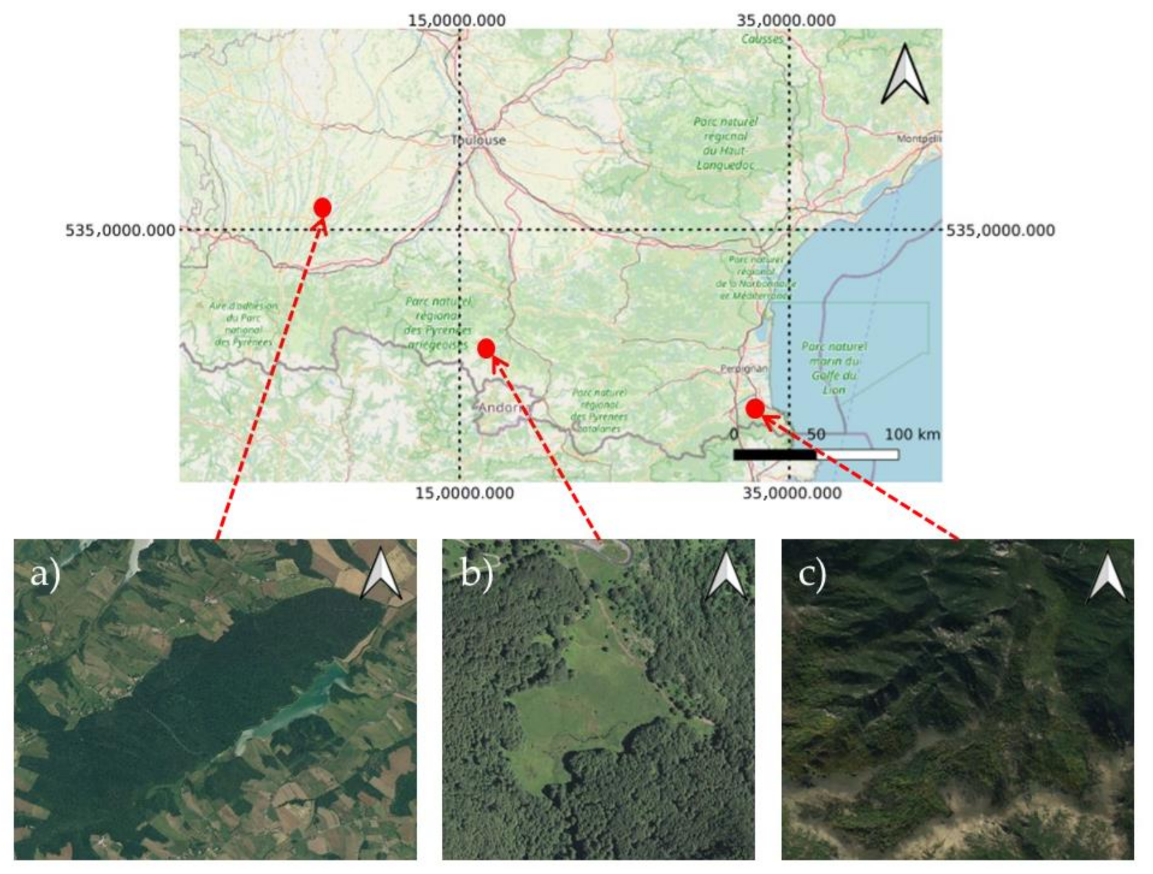
2.1. Study Sites

Three sites located in southwestern France with different species diversity were selected for this study (Figure 1). The first site is the Suc-et-Sentenac national forest surrounding the Bernadouze peat bog, part of the “Haut-Vicdessos” Human-Nature Observatory located in Ariège (French Pyrenees), supported by the French CNRS and the LabEx DRIIHM [39]. This is a long-term study site where hydrological, climatological, botanical, archeological, remotely sensed surveys are monitored regularly. This natural forest is mainly composed of beech with some conifers. The site covers about 23 ha and the mean altitude is around 1500 m asl.

The second site is the Fabas forest located in the “Vallées et Coteaux de Gascogne” (Haute-Garonne, France), belonging to the ZA PYGAR long-term socio-ecological research site (LTSER) [40]. It covers about 550 ha of hilly terrain with an average altitude of 371 m asl. This forest was extensively reforested between 1968 and 1975. The majority of trees are coniferous species, including Douglas fir, Corsican pine, maritime pine, black pine and silver fir. It only contains marginal numbers of broadleaf species, mainly oak but also locust. Over the years, this site has become very heterogeneous with reserve oak trees in conifer plantations.

The third site is the forest of La Massane National Nature Reserve [41], located in the eastern part of the Albères massif (Pyrénées-Orientales, France). The forest extends over 336 ha between 600 and 1150 m asl. Considered as one of the 40 last old-growth forests in the Mediterranean basin, this forest was recently classified as a UNESCO World Heritage site. It is a biodiversity hotspot with 6467 species of flora and fauna including 23 tree species. The main tree species, i.e., represented by more than 10 trees per hectare, are beech and pubescent oak. Some maples, alders, black pines, cherry woods, holm oaks and white birch are scattered across the site.

2.2. Data Acquisition and Preprocessing

The LiDAR data were acquired over the Bernadouze forest on 5 September 2014, at 11.15 a.m. UT (Universal Time), at 3245 m above sea level under scattered cloud conditions, using an Optech 3100EA sensor (wavelength: 1064 nm, spot diameter: 0.8 m, point density: 3 pts/m²). The data were processed by the French National Mapping Agency IGN and the French Aerospace Lab (ONERA) using TerraSolid software (@TerraSolid Ltd., 02600 Espoo, Finland) and the open-access SPDLib library to generate a CHM with 1 m spatial resolution [43,44]. On 12 September 2014, an airborne hyperspectral image was acquired at the same flying height and the same sky conditions as the LiDAR data, using a VNIR-1600 HySpex sensor (Norsk Elektro Optikk AS, Lørenskog, Norway) with 1 m ground spatial resolution and 3.6 nm spectral resolution in the VNIR (visible near-infrared spectral range [400:1000] nm) domain (160 spectral bands) (

Table 1. Image dataset description per site.

Site	Spectral Image 1	CHM 2	Forest Type 3
Bernadouze	HS 4-VNIR-1 m	1 m	Mono-species (beech)
Fabas	HS 4-VNIR-1 m	1 m	Mixed-species (five major species, two types: deciduous and coniferous)
La Massane	RGB-Visible-0.1 m	0.5 m	Mixed-species (23 species, but the majority beech, one type: deciduous)

¹ (Type-spectral range-spatial resolution), ² Spatial resolution, ³ Mono- or mixed-species, ⁴ HS = Hyperspectral.

). The surface reflectance image was retrieved from the georeferenced radiance image using the Cochise tool [45].

For the Fabas forest, a LiDAR point cloud was acquired in May 2016 with a Riegl LMS Q680i during the MUESLI project (MUltiscale mapping of Ecosystem Services by very high spatial resolution hyperspectral and LiDAR remote-sensing Imagery, funded by the University of Toulouse [46]). The flying height of the LiDAR acquisition was 600 m above the ground and the point density was about 4 points/m². The point coordinates were computed using RiAnalyze and RiWorld (Riegl) software. DSMs (digital surface models) and DTMs (digital terrain models) were generated from this point cloud using TerraSolid software. The difference between the DSM and the DTM provided the CHM in raster format with a 1 m spatial resolution. Airborne hyperspectral images were acquired over the Fabas forest on 15 September 2015 at 8:07 UT with a HySpex VNIR-1600 camera system. The flying height was approximately 1287 m above this site under clear sky conditions. After geometric and atmospheric corrections, the images obtained represented top-of-canopy spectral reflectances with a spatial resolution of 1 m in the VNIR domain (Table 1).

The LiDAR dataset was acquired over La Massane forest site on 19 May 2016 with a Riegl LMS Q680i 600 m above the ground, with an averaged point density of 56 points/m². After preprocessing, the CHM was generated with 50 cm spatial resolution. The spectral data used for this forest site were ORTHO HR^® (high-resolution orthophotography), provided by the IGN, composed of aerial RGB images with a 10 cm spatial resolution, acquired on 19 April 2016 (Table 1).

2.3. Training and Testing Datasets

A reference dataset was built for each site (

Table 2. Description of the reference dataset per site.

Study Area	Tree Crown Number	Mean Crown Area (m2)	Description	Data Used for Photo-Interpretation
Bernadouze	96	73	Different locations in the forest and different crown sizes	CHM (1 m) BD ORTHO® (0.5 m)
Fabas (entire site)	449	75	Tree types (coniferous/broadleaf) and species spatial distribution (mixed/monospecific)	CHM (1 m) BD ORTHO® (0.5 m)
Fabas (test area)	200	58	Tree types (coniferous/broadleaf) and species spatial distribution (mixed/monospecific)	CHM (1 m) BD ORTHO® (0.5 m)
La Massane	200	60	Tree species, different locations and crown sizes	CHM (0.5 m) BD ORTHO® (0.1 m)

) by photointerpretation. Crowns were manually segmented using CHM and orthophotography with a high spatial resolution to be sure the geometrical information was accurate. Crown locations were referenced by computing the centroid of each crown segment. The reference crowns were distributed over each study area, with different characteristics related to their location in the forest (in the heart and/or at the edge of the forest), tree geometry (crown size and shape), tree type (coniferous/broadleaf, mixed/mono-species) and observation conditions (shaded surface) (Table 2). The reference dataset was built respecting a balance between the different classes (especially coniferous/broadleaf species) and covering the entire forest sites homogeneously. The reference database was randomly divided into two parts: the training set used to optimize input parameters was composed of 50% of the polygons and the validation set used to assess performance included the remaining 50%. Ten random splits were performed to ensure robust results.

Figure 2 presents the structural characteristics of the crowns at the three forest sites, estimated using the reference dataset. The maximum height corresponds to the maximum value of the CHM within a tree crown. The second characteristic is related to the difference between the maximum and minimum values of the CHM within a tree crown. The third characteristic corresponds to the tree crown radius. Each site has specific crown characteristics:

• The maximum heights in La Massane forest are relatively shorter than at the two other sites,
• Two modes were identified in the radius histogram for Fabas forest, corresponding to coniferous and broadleaf species.

These characteristic differences highlight the need to develop an adaptive method.

The Bernadouze dataset was used to represent different tree locations in a mono-species forest; it includes 59 tree crowns on the forest edge and 37 crowns in the heart of the forest. These two tree locations explain the two modes identified in the maximum height histogram in Figure 2. Trees at the forest edge have a lower height than trees in the heart of the forest.

The Fabas dataset includes 233 broadleaf trees and 216 pines. Of the broadleaf trees, 170 are located in mixed stands (pine and broadleaf trees). Of the pines, 184 are located in mixed stands. The shadow represents 39% of the pixels in the crowns due to the early acquisition time and relief slopes. The Fabas forest was divided into three areas to reduce the data volume and processing time. Each area was characterized by a specific tree distribution (

Table 3. Fabas forest: Tree-type characteristics (numbers of reference tree crowns). N/A, not acquired at the site concerned.

	Coniferous (Mono-Type Area)	Coniferous (Mixed Area)	Broadleaf (Mono-Type Area)	Broadleaf (Mixed Area)
Bernadouze (23 ha)	N/A	N/A	98	N/A
La Massane (52 ha)	N/A	N/A	200	N/A
Fabas
Area 1 (155 ha)	32	34	31	35
Area 2 (160 ha)	N/A	41	32	44
Area 3 (235 ha)	N/A	109	N/A	91
Total	32	184	63	170
Test area (11.6 ha)	65	80	30	25

). A small extract of Fabas forest, called the test area, was used to calibrate the method of delineation. The area covered 11.6 ha and contained the same proportions of coniferous and broadleaf species as the whole site (Table 3).

Figure 3 presents the structural characteristics of the crowns of broadleaf and coniferous species in the Fabas test area. The main differences in radius (about 3 m) and height (about 5 m) between the two types of trees underline the need to adapt the method of delineation to the type of tree.

The La Massane dataset comprised 200 crowns of broadleaf species. This dataset was completed by a ground inventory including species identification and DBH provided by ecologists.

2.4. MCG-Tree Method

The MCG-Tree (multi-criteria graph) method provides a tree crown delineation map. Figure 4 presents the four main steps of the MCG-Tree method. The inputs are CHM and optical images (hyper- or multi-spectral images, ortho-photography). The method is based on an initial watershed segmentation of the CHM.

This initial segmentation map is transformed into a graph where a segment corresponds to a node and links to its neighbors [33]. This permits grouping segments belonging to the same crown [33]. This step is achieved by applying spectral and geometric criteria, followed by thresholding.

Spectral information is introduced to complete the geometric criteria at different levels of the MCG-Tree method:

• During preprocessing, to mask the shadowed pixels;
• During graph processing, to merge segments belonging to the same tree;
• During post-processing, to classify the tree type to adapt the geometric criteria.

The spectral parameters of these three levels are detailed in the following paragraphs. When optical images are not available, the MCG-Tree method applies geometric criteria to produce a graph and the shadowed pixels are not masked.

The MCG-Tree method is implemented with the scipy [47], scikit-learn [48] and scikit-image [49] python packages.

2.4.1. Preprocessing

A global mask is generated by combining a vegetation mask and a shadow mask. The vegetation mask is obtained by thresholding each pixel of the CHM to select pixels corresponding to the tree layer. In this work, the height threshold was set to 2 m to mask pixels corresponding to bare soil and low-growing plants. The shadow mask was computed from the hyper or multi-spectral images. Considering blue, green, red and near-infrared (NIR) spectral bands (respectively 480, 550, 670 and 780 nm), the following formulation was applied to produce a composite image [50]:

$$1/6\left(2\mathrm{blue}+\mathrm{green}+\mathrm{red}+2\mathrm{NIR}\right)$$

A threshold in reflectance was applied to the composite image. The value of this threshold is evaluated in Section 3.1.1. When no hyper or multi-spectral image is available, the global mask represents only the vegetation mask.

A median filter was applied to the CHM to reduce the noise while maintaining sharp edges. The optimal size of the filter is defined in Section 3.1.1.

A combination of three spectral bands to enhance the spectral information was selected to compute the spectral characteristics and define the spectral criteria to cut the graph (Figure 4). To reduce the processing time, only three spectral bands were selected, following the study by Lee et al. [31]. Two spectral band combinations were tested and compared:

• RGB bands at 480, 550 and 670 nm, a standard combination that is often accessible by passive optical remote sensing.
• A combination of the first components of principal component analysis (PCA) was applied to the hyperspectral image [51]. This improves the interpretability by creating uncorrelated features with maximized variance [52].

2.4.2. Initial Segmentation (Reference Map)

In the present study, the initial segmentation was obtained using the watershed method applied to the CHM, using the local maxima as seed points [33]. This map was used as the reference map to compare the ITC maps.

2.4.3. Graph Generation and Parameter Computation

A graph was produced to improve segmentation by merging segments belonging to the same crown, using geometric and spectral criteria. The graph permitted the application of criteria to each segment and comparison with neighbors [53]. The initial segmentation map was converted into a graph where each segment corresponded to a node and was connected to its neighbors by links.

The geometric characteristics related to the CHM are the maximum height value and the location of the pixels of maximum height. The spectral characteristic is the mean spectral value from RGB or PCA image bands. Each spectral or geometric characteristic is computed at each node of the graph.

Several parameters are deduced from these characteristics at each link that connects two nodes. In

Table 4. List of MCG-Tree parameters.

Method Steps	Parameters
Preprocessing	Shadow mask threshold
	Median filter size
Graph generation/Segment clustering	Difference in height between the maximum heights ∆hmax
	Planar Euclidian distance between the maximum heights dhmax
	Local height variation between the maximum heights ∆hloc
	∆spec (on RGB image or three first components of ACP)

, the list of MCG-Tree parameters reports the different parameters we used in the MCG-Tree method. They are defined so as to distinguish crown characteristics. Then, for each link, the four following parameters are selected (Figure 5):

• Difference in height between the maximum heights of two adjacent nodes (∆h_max);
• Planar Euclidian distance between the maximum heights of two adjacent nodes (dh_max);
• Local variation in height corresponding to the difference in height between the maximum and minimum values on a transect connecting the maximum heights of two adjacent nodes (∆h_loc),
• Euclidian distance between mean spectral values of two adjacent segments (∆spec).

2.4.4. Segment Clustering

The previous parameters were used to merge segments corresponding to the same tree crown based on a voting approach. Each parameter (∆h_max, dh_max, ∆spec and ∆h_loc) was independently compared to a threshold. If the parameter value was higher than the threshold, the vote is positive; otherwise, it was negative. If the majority of votes were negative, the link between the two nodes being compared was cut; otherwise, the link was conserved. This operation was applied to every link of the graph. Once this process was complete, nodes that remained linked were merged, giving the final delineation map. Figure 6 illustrates the different graph-cut and segment-merging steps of the MCG-Tree method.

The thresholds of all the parameters were automatically trained using the characteristics of the forest under study, to obtain the optimal parameter values. For each parameter, the value interval was set according to forest characteristics (Section 2.3):

• Variations in tree height in the forest canopy were used to set the ∆h_max and ∆h_loc intervals;
• The overall shape of the tree crown defined the dh_max interval;
• Spectral variation among tree types was used to set the ∆spec interval.

All the combinations of the parameter values set in these ranges were then assessed on a training set. The optimal combination of values defined the thresholds used to process the whole forest site.

2.4.5. Automatic Adaptation of the MCG-Tree Method According to the Type of Tree

At this point, the MCG-Tree method did not account for differences in the characteristics between coniferous and broadleaf species in one forest site and a single set of parameters was applied to the entire site. Consequently, automatic adaptation of the MCG-Tree method according to the tree type was applied if a hyper or multi-spectral image was available. In this study, we only applied this adaptation to Fabas forest, which is a mixed forest.

A delineation map was produced for each tree type (coniferous, broadleaf). The geometric parameter thresholds were then set according to the tree type (Section 3.1.2). To this end, a preliminary step was required to distinguish coniferous from deciduous trees using passive imagery. This mask was incorporated in the method to automatically merge the delineation maps according to the tree type (Figure 7).

The tree types were classified independently of the delineation using Random Forest (RF), a widely used machine-learning algorithm [54]. We used the RF algorithm in the scikit-learn python package [48]. After classification, cascaded individual median and erosion/dilatation filters were applied to the resulting map to obtain homogeneous patches of classes [55]. Each segment of the delineation maps was superposed on the classification map. If a segment of the delineation map adapted to a certain tree type contained a majority of pixels classified as this tree type, the segment was kept on the merged delineation map.

2.5. Performance Assessment

The performance was assessed by comparing the resulting tree crown and the reference ITC [18,23,26]. The accuracy of delineation was expressed in terms of one of the following categories [18] (Figure 8):

• Matched—The reference ITC recovered more than 50% of a segment and this segment recovered more than 50% of the validation ITC;
• Missed—The reference ITC did not recover more than 50% of any segment;
• Over-segmented—The reference ITC recovered more than 50% of several segments;
• Under-segmented—A segment recovered more than 50% of the reference ITC but the reference ITC did not recover more than 50% of the segment.

The number of correctly delineated crowns required to assess the global performance ratio was the number of matched cases normalized by the total number of reference ITCs.

3. Results

This section is divided into two parts. The first section concerns the calibration step to produce the optimal parameter sets. The second section presents the multi-site application of the approach together with its performance.

3.1. Calibration Step

All the parameters listed in Table 4 have an impact on delineation results. In this section, these parameters are optimized on the Fabas test area. A sensitivity analysis of those key parameters is reported. The input parameters differ depending on the tree type. Their sensitivity to the tree type and their influence on the overall delineation performance are analyzed before we present an automatic adaptation of the MCG-Tree method to the tree type.

3.1.1. Optimal Input Parameter Values

Shadow Mask Threshold

The impact of the shadow mask on delineation performance is illustrated in Figure 9. The other MCG-Tree parameters are set at optimal values estimated empirically (median filter window = 3 × 3 pixels, dh_max = 3.5 m and ∆h_loc = 0.6 m). It is important to note that these parameters are adapted to an application regardless of the tree type.

The shadow threshold impacts the delineation performance of the reference and MCG-Tree methods, especially in the case of coniferous trees. The selected threshold is set to 0.035, which produces the best performance for coniferous species (delineation performance: 0.78) and for all trees whatever the type (performance: 0.81). Figure 9 also shows that the MCG-Tree method mainly improves the performance for broadleaf species compared to coniferous ones. The fact that broadleaf trees have bigger crowns than coniferous species results in more over-segmented cases in the watershed segmentation. The MCG-Tree, which corrects over-segmented cases, thus has more impact on the crowns of broadleaf trees.

CHM Median Filter Size

Figure 10 shows the assessment of delineation performance for four window sizes of the median filter (2 × 2, 3 × 3, 4 × 4 and 5 × 5), with the other parameters set to the following values: 0.035 for the shadow mask threshold, 3.5 m for dh_max and 0.6 m for ∆h_loc.

With the reference method, the optimal filter size depends on the tree type. The best performance is obtained:

• For the coniferous type, with a 2 × 2 window size;
• For the broadleaf type, with a 4 × 4 window size;
• For all trees, with a 3 × 3 window size.

With the MCG-Tree method, a 3 × 3 window size produces the best results in all cases. This method has the advantage of fixing the median filter size to a single value in comparison to the reference method. The 2 × 2 window size is useful because it leads to marked over-segmentation on the initial delineation map, perfectly suited to areas with narrowed trees in planted coniferous forests. However, Figure 10 does not show the improved performance for coniferous species with the MCG-Tree method even with a 2 × 2 median filter size because the parameter that is set was chosen to be suitable for global application. This filter size will be further investigated in monospecific coniferous stands with a suitable set of parameters (dh_max, ∆h_loc). The 3 × 3 window size of the median filter is used for application to the whole forest site.

Single-Criterion Analysis

The influence of each MCG-Tree criterion on delineation performance is evaluated. This enables identification of the optimal combination of criteria for the following application to all of the forest sites.

The shadow mask threshold is set to 0.035 and the median filter window size 3 × 3. These parameters give a delineation performance of 0.71 using the watershed reference method.

The threshold value for each geometric and spectral parameter varies (Section 2.4.3) and the delineation performance of the MCG-Tree method is assessed for each threshold. Figure 11 shows the impact of each geometric or spectral criterion threshold on the delineation performance.

Up to a specific value, the dh_max and ∆h_loc parameter thresholds improve the delineation performance. The best results are obtained with the following thresholds: dh_max 3.5 m (performance 0.76) and ∆h_loc 1.1 m (performance 0.79). Analyzed individually, the ∆spec and ∆h_max parameters reduce the delineation performance. ∆spec is estimated over RGB bands or the three first PCA components. As shown in Figure 11, the drop in performance caused by ∆spec is smaller with PCA than with RGB band selection. Owing to their specific impact on performance, dh_max and ∆h_loc are only kept for the following sensitivity analysis.

Multiple-Criterion Analysis (Vote Assessment)

Application of the MCG-Tree method criteria is based on a voting approach that combines criteria. The dh_max and ∆h_loc criteria were analyzed separately in the previous section. Here, the thresholds of the criteria dh_max and ∆h_loc are varied simultaneously to identify the optimal value pair that produces the best-quality delineation. The ranges of variation of the dh_max and ∆h_loc thresholds are 0–7 and 0–2, respectively. With a sampling interval of 0.5 for dh_max and 0.1 for ∆h_loc, the best performance of 0.81 is obtained with the following values: dh_max threshold set to 3.5 m and ∆h_loc threshold equal to 0.6 m (Figure 10).

3.1.2. Calibration According to Tree Type

Range of Input Parameters According to Tree Type

The tuning of MCG-Tree geometric parameters according to the tree type is analyzed by simultaneously evaluating dh_max and ∆h_loc. The ranges of variation of the dh_max and ∆h_loc thresholds are the same as in Section 3.1.1. The number of over-segmented and under-segmented cases is analyzed for each type. The optimal median filter size is 2 × 2 for coniferous species and 3 × 3 for broadleaf species.

Table 5. Best delineation performance for coniferous and broadleaf trees obtained in the Fabas forest test area.

	Median Filter Size	dhmax	∆hloc	P 1	Matched	Missed	O-S 2	U-S 3
Coniferous	2 × 2	[0.5–2]	[0.1–0.9]	0.80	116	0	0	29
Broadleaf	3 × 3	[3,4,5]	[0.5–1.1]	0.93	51	0	2	2

¹ Performance, ² Over-segmentation, ³ Under-segmentation.

lists the combinations of geometric criteria selected for each tree type. For each parameter, the performance of all the values included in the initial range is equivalent. The number of cases of over-segmentation is low for both tree types. There are more cases of under-segmentation for coniferous species, even though the median filter window size is optimal for this type, due to the small crown radius and the proximity of neighboring trees.

The selected optimal values of the geometric parameters depend on the characteristics of each tree type (Figure 3). The range of dh_max thresholds that produce the best results for each tree type (Table 5) is linked to the tree crown radius in the test area (around 3 m for coniferous and 5 m for broadleaf trees). Crowns of coniferous trees usually have a smaller radius than the crowns of broadleaf trees. The best delineation performance is thus obtained for the coniferous type with a lower dh_max threshold value (performance 0.80). The dh_max values listed in Table 5 are slightly lower than the mean crown radius (Figure 3). In fact, the distance between two segments located in an over-segmented tree crown is slightly shorter than this crown radius.

Criterion ∆h_loc is linked to the difference between the maximum and minimum heights of the tree crowns (Figure 3). This characteristic depends only to a slight extent on the tree type, which is why the ∆h_loc intervals giving the best results for each tree type are similar (around 0.7 m).

Automatic Adaptation of MCG-Tree Method

The automatically adaptable version of the MCG-Tree method is applied to distinguish coniferous from deciduous trees. To provide a complete tree type (coniferous and deciduous) cartography, 50% of the ITCs delineated by photo-interpretation are used for RF training and 50% to assess the accuracy.

A median filter (4 × 4 window) and a dilatation/erosion filter are applied to the classification map to select homogeneous coniferous and broadleaf regions. The resulting overall accuracy of the classification is 0.87. Different dilatation and erosion filters ranging between 1 and 10 in size are tested. The best classification map is obtained with a size 5 dilatation filter followed by size 2 erosion.

The resulting classification map is then used as a mask to merge the two delineation maps obtained for the coniferous and broadleaf types and results in a global delineation performance of 0.83. The adaptation of MCG-Tree parameters according to the forest type slightly improves the delineation performance with an increase of around 2% compared to previous results (Figure 10, performance around 0.81).

3.2. Performance of the MCG-Tree Method

Table 6. Best global delineation performance obtained for each forest site using the MCG-Tree method and the reference method.

	Median Filter Size	dhmax	∆hloc	P Reference	P MCG-Tree
Fabas
Area 1	3 × 3	[0.5–2.5]	1	0.76	0.82
Area 2	3 × 3	[0.5–3.5]	[1.5–1.6]	0.61	0.75
Area 3	3 × 3	[0.5–2.5]	1.6	0.59	0.73
All	3 × 3	[0.5–2.5]	[1.5–1.6]	0.65	0.76
Bernadouze
	3 × 3	4.5	[0.7–1.3]	0.45	0.70
La Massane
	3 × 3	3	1	0.61	0.72

lists the results obtained for the three forest sites. The input parameter intervals are set according to the calibration stage presented previously (Section 3.1.2). The MCG-Tree method performance is compared to that of the reference method. The values or intervals reported for each parameter in the table correspond to the optimal sets giving the best delineation performance for each forest site.

Following the results in Section 3.1.1, the median filter size is set to 3 × 3 pixels whatever the tree type. The ranges of variation in the parameters defined in Section 3.1.2 are evaluated.

The best performance is obtained for the Fabas forest test area, which contains more coniferous trees and less crown overlap between trees. Whatever the forest site, the MCG-Tree method improves the delineation performance compared to the classical watershed method. The biggest improvement is achieved for Bernadouze forest (around 0.25 the global performance). The least improvement was achieved for Fabas forest area 1 (0.057), containing the largest area of monotype coniferous trees, leading to low over-segmentation cases after watershed application. In this case, the MCG-Tree method only enables limited improvement. Figure 12 shows examples of delineation results for the three forest sites. The MCG-Tree method has more impact on the two broadleaf forests (Bernadouze and La Massane) because of the presence of more cases of watershed over-segmentation on broadleaf tree crowns. Overall, the disparity (difference between best and worst performance) in the delineation performance in all three forest sites is lower with the MCG-Tree method (0.12) than with the reference method (0.31). Our method provides the most homogeneous performance when applied to more than one site.

Figure 2 shows tree crown characteristics according to each forest site. The comparison between these tree crown characteristics and MCG-tree method criterion thresholds (Table 6) confirms that dh_max can be defined using the crown radius. The relationship between the ∆h_loc threshold and the difference in maximum height versus minimum height is more ambiguous. This characteristic was very similar at the three sites and explains why the optimal ∆h_loc threshold value is similar for each site. A ∆h_loc threshold in the range of 1–1.6 m seems to be a good tradeoff regardless of the forest site concerned. To conclude, the MCG-Tree method leads to an improvement of between 0.057 and 0.25 compared to the reference method.

4. Discussion

4.1. Benefit of Spectral Information for Tree Crown Delineation

The spectral criterion (∆spec) has a negative impact on the correction of over-segmented crowns. Lee et al. proposed a similar graph approach with spectral information from hyperspectral data processing and structural information extracted from LiDAR data. The feature space of hyperspectral imagery was reduced using PCA to delineate tree crowns, and adding spectral information with LiDAR data (six points per m²) reduced the performance [31]. Although spectral signatures can identify edges between two crowns of different species, segmentation errors are often detected between the same type of tree (especially overlapping crowns between broadleaf trees). This explains the limited benefit of spectral parameters when LiDAR-based delineation is added, especially in monospecific forests with similar spectral signatures. It is also important to take into account the registration error when different kinds of data are combined. In our case, the registration error is lower than the pixel resolution, but in the future, it will be interesting to check the robustness of the method to registration error by sensitivity analysis.

The shadow mask permits removing noise due to the shadow. This improves the delineation performance by enhancing the information of interest used by the segmentation method. The present study showed that shadow between tree crowns has a greater impact on delineation quality than spectral criteria. For this study, a simple shadow mask based on intensity thresholding was implemented. An optimal shadow mask threshold was set by taking the solar angle linked with time acquisition, spacing between trees, tree heights and relief of the study site into account. These characteristics influence the extent of the shadow area, which in turn, has a direct impact on delineation performance, for example, by affecting the number of pixels taken into account for each crown. An automatic shadow-thresholding calculation has been developed and can be adapted for application to forests, provided that geometric and spectral data are correctly georeferenced [56]. The combined use of spectral-based (histogram thresholding) and geometrical-based (ray tracing) methods could enable very precise shadow detection.

4.2. Advantage of Geometric Information for Tree Crown Delineation

The watershed algorithm tends to over-segment large trees [31] but this behavior can be controlled by two specific geometric criteria, dh_max and ∆h_loc. These criteria are related to tree crown structural characteristics that can be estimated in advance using local in-field measurements or photo-interpretation, to adapt MCG-Tree thresholds to the forest site under study, to enhance delineation performance. Estimating a mean crown radius makes it possible to define an optimal dh_max threshold value. The definition of ∆h_loc is more complex, but in this study, the optimal interval threshold values obtained for the three sites were similar (between 1 and 1.6 m).

Estimating parameter thresholds related to the crown characteristics is a promising way to apply the method to other sites. However, this threshold estimation is based on prior knowledge of the general characteristics of the forest and can be optimized. For example, the sequential forward floating selection approach may provide the optimal combination of criteria to distinguish distinct crown segments [57].

In this paper, the crown radius was used to define criteria, but complementary metrics can also be used. For example, some authors compute tree crown characteristics from LiDAR point clouds (point density, crown shape, intensity of points, leaf area index—LAI, etc.) to enhance delineation [58,59]. The MCG-Tree method produced good results for the three forest sites, using low-density point clouds derived into a CHM, but a density higher than the one used in our study (Bernadouze and Fabas forest sites) is usually required to effectively compute tree crown characteristics from a point cloud. The method proposed by Strîmbu et al. used graph hierarchy as a criterion to evaluate whether two segments belong to the same crown with a 30 points/m² LiDAR density [58]. New criteria were then calculated directly from a 3D point cloud based on tree structure detection or variation in density. Some recent tree-detection studies based on 3D point clouds with different point densities (from 10 to 200 points/m²) produced good results, especially for stem detection, which can be a useful parameter for crown delineation [60,61]. These criteria based on high-density point clouds could be integrated to improve delineation performance and to suit other applications like standing dead-tree delineation [62] or the detection of understory trees [34].

4.3. Automatic Adaptation in the Case of a Mixed Forest

In the case of mixed forest, the structural characteristics differ between coniferous and broadleaf trees (Figure 3). MCG-Tree criteria need to be locally adaptable to obtain the best results. In this study, supervised classification (RF method) was applied to discriminate between coniferous and broadleaf trees, as we introduced into the delineation process. The results showed a slight increase in global delineation performance in the Fabas forest test area. However, the performance decreased for the entire site versus that obtained with a single criterion. This result is due to the very mixed appearance of Fabas forest, where some broadleaf trees are surrounded by a large number of coniferous trees, thus requiring more precise mapping of the two types of trees. Classification combining the CHM texture and hyperspectral data improved the initial classification closest to the edges of delineation segments as defined in the CHM. It also made it possible to increase the classification to more than two classes.

The adaptability of MCG-Tree criteria also varies with the amount of over-segmentation. Coniferous trees with a smaller crown radius than broadleaf crowns need a smaller segment size. On the contrary, too many segments in a large broadleaf tree crown lead to over-segmentation. One way to control the over-segmentation obtained by initial watershed segmentation is to adapt the size of the CHM median filter window according to the tree type. Our results show that a 2 × 2 median filter size is optimal for coniferous trees with a 3-m crown radius and a 1-m CHM resolution. For broadleaf trees with a 5-m radius, a 3 × 3 median filter size produces the best results. Another way to adapt over-segmentation would be to adapt the CHM spatial resolution, as some studies showed that the CHM resolution influenced the delineation performance [26,63]. In the presented study, the CHM of La Massane had a higher spatial resolution than the other sites. The higher pixel number in a unique tree crown leads to more important intra-crown variation, which generates more cases of over-segmentation (Figure 12). Identifying the optimal CHM resolution according to tree crown size would make it possible to determine the data properties (LiDAR point density, optical data resolution, etc.) best suited to each forest site.

4.4. MCG-Tree Adaptability to Multi-Sites

The results for the delineation of mixed and coniferous forests were generally better than those for deciduous forests. The delineation of Fabas forest (mixed forest) was better than that of Bernadouze forest (beech forest) and La Massane forest (multi-species broadleaf dominant forest) using the MCG-Tree method. This result is in agreement with some studies that compared results for delineation of different tree types [18,64,65]. However, in addition, our method is able to adapt criteria based on crown characteristics related to the tree type, thereby reducing the disparity between different forest applications.

High recovery between neighboring tree crowns is a real difficulty in distinguishing broadleaf ITC. The use of point clouds with a high point density could make it possible to link variations in the canopy to individual tree trunks, thereby improving broadleaf tree delineation [59]. Application to forest sites with different characteristics is necessary to evaluate the adaptation of the method [16,18]. Few authors applied their methods to more than one forest site [16]. Lee et al. obtained mitigated results when working on coniferous- or broadleaf-dominated forests [31]. Spectral and geometric variability between forest sites due to the presence of different species and/or tree spatial distribution (mixing rate) and/or the presence of shadows makes it difficult to rely on a single delineation method. That is why in this study, we explored an adaptive approach based on crown characteristics specific to the forest site under study. This approach now requires further study to develop operational delineation methods.

5. Conclusions

The MCG-Tree method consists of a graph-based approach using multiple geometric and spectral criteria to correct over-segmentation on an initial watershed delineation map, used as a reference map to quantify performance. Our method was applied to three temperate forest sites with different characteristics (mixed forest, mono-species broadleaf forest and a mainly multi-species broadleaf forest) using CHM with different spatial resolutions (0.5–1 m) and several optical data (hyperspectral and BD ORTHO^® RGB). The MCG-Tree method improved the overall performance in the three forest sites by up to 25% compared to the reference watershed method.

Our method combines spectral and geometric criteria and is able to add new criteria if required. Criteria evaluation showed that only two geometric criteria (dh_max and ∆h_loc) are needed to correct over-segmentation. One is directly related to the tree crown radius, and the optimal corresponding threshold value can be defined before the method is applied using tree crown information estimated for the study sites concerned. Shadow masks deduced from optical images also influenced delineation performance.

Tree crown characteristics of mixed forests containing both coniferous and broadleaf species vary considerably. A preliminary step to classify the tree type was thus added to automatically adapt MCG-Tree criteria to the tree type. Promising results were obtained in a small area but further investigations of tree-type classification at larger scales are required. Adapting the delineation to the tree type involves controlling over-segmentation, for example, by modifying the CHM median filter size. For a 1-m spatial resolution of CHM, a 2 × 2 median filter size is optimal for coniferous tree crowns with a radius of 3 m, and a 3 × 3 median filter size is optimal for broadleaf tree crowns with a radius of 5 m.

In this study, only the raster CHM was used to compute geometric criteria characterizing tree crowns. Using new criteria based on the tree structure derived from high-density (>10 points/m²) LiDAR point clouds could make it possible to detect more complicated structures like understory trees or dead standing trees.

Delineation tree crown maps can be used for forest management or tree resource evaluation. In future work, delineation will be the first step before species classification at the tree scale using airborne hyperspectral data. Object-based classification using delineated tree crowns as the input will be compared to a pixel-based approach.

References

1. European Environment Agency rapport on Forest Dynamics in Europe and their Ecological Consequences. Available online: https://www.eea.europa.eu/themes/biodiversity/forests (accessed on 27 October 2021).
2. Brown, S.; Sathaye, J.; Cannell, M.; Kauppi, P. Mitigation of carbon emissions to the atmosphere by forest management. Commonw. For. Rev. 1996, 75, 80–91. [Google Scholar]
3. Beguin, J.; Tremblay, J.P.; Thiffault, N.; Pothier, D.; Côté, S. Management of forest regeneration in boreal and temperate deer–forest systems: Challenges, guidelines, and research gaps. Ecosphere 2016, 7, e01488. [Google Scholar] [CrossRef]
4. IGN Study of Forest Wood Availability in Occitanie Region. Available online: https://inventaire-forestier.ign.fr/IMG/pdf/rapport_occitanie_phase_i.pdf (accessed on 27 October 2021).
5. Reddy, C.S.; Kurian, A.; Srivastava, G.; Singhal, J.; Varghese, A.O.; Padalia, H.; Rao, P.V.N. Remote sensing enabled essential biodiversity variables for biodiversity assessment and monitoring: Technological advancement and potentials. Biodivers. Conserv. 2020, 30, 1–14. [Google Scholar] [CrossRef]
6. Pereira, H.M.; Ferrier, S.; Walters, M.; Geller, G.N.; Jongman, R.H.G.; Scholes, R.J.; Wegmann, M. Essential biodiversity variables. Science 2013, 339, 277–278. [Google Scholar] [CrossRef] [PubMed] [Green Version]
7. Dobbertin, M. Tree growth as indicator of tree vitality and of tree reaction to environmental stress: A review. Eur. J. For. Res. 2005, 124, 319–333. [Google Scholar] [CrossRef]
8. Achard, F.; Hansen, M.C. Global Forest Monitoring from Earth Observation; Taylor & Francis: Abingdon-on-Thames, UK, 2012. [Google Scholar]
9. Skidmore, A.K.; Coops, N.C.; Neinavaz, E.; Ali, A.; Schaepman, M.E.; Paganini, M.; Wingate, V. Priority list of biodiversity metrics to observe from space. Nat. Ecol. Evol. 2021, 5, 896–906. [Google Scholar] [CrossRef] [PubMed]
10. Zhang, W.; Ke, Y.; Quackenbush, L.J.; Zhang, L. Using error-in-variable regression to predict tree diameter and crown width from remotely sensed imagery. Can. J. For. Res. 2010, 40, 1095–1108. [Google Scholar] [CrossRef]
11. Heinzel, J.; Koch, B. Investigating multiple data sources for tree species classification in temperate forest and use for single tree delineation. Int. J. Appl. Earth Obs. Geoinf. 2012, 18, 101–110. [Google Scholar] [CrossRef]
12. Maltamo, M.; Næsset, E.; Vauhkonen, J. Forestry applications of airborne laser scanning. Concepts Case Stud. Manag. Ecosys 2014, 27, 2014. [Google Scholar]
13. Lechner, A.M.; Foody, G.M.; Boyd, D.S. Applications in remote sensing to forest ecology and management. One Earth 2020, 2, 405–412. [Google Scholar] [CrossRef]
14. Lim, K.; Treitz, P.; Wulder, M.; St-Onge, B.; Flood, M. LiDAR remote sensing of forest structure. Prog. Phys. Geogr. 2003, 27, 88–106. [Google Scholar] [CrossRef] [Green Version]
15. Lindberg, E.; Holmgren, J. Individual tree crown methods for 3D data from remote sensing. Curr. For. Rep. 2017, 3, 19–31. [Google Scholar] [CrossRef] [Green Version]
16. Zhen, Z.; Quackenbush, L.J.; Zhang, L. Trends in automatic individual tree crown detection and delineation—Evolution of LiDAR data. Remote Sens. 2016, 8, 333. [Google Scholar] [CrossRef] [Green Version]
17. Hanapi, S.S.; Shukor, S.A.A.; Johari, J. A Review on Remote Sensing-based Method for Tree Detection and Delineation. In IOP Conference Series: Materials Science and Engineering; IOP Publishing: Bristol, UK, 2019; Volume 705, p. 012024. [Google Scholar]
18. Hastings, J.H.; Ollinger, S.V.; Ouimette, A.P.; Sanders-DeMott, R.; Palace, M.W.; Ducey, M.J.; Orwig, D.A. Tree species traits determine the success of LiDAR-based crown mapping in a mixed temperate forest. Remote Sens. 2020, 12, 309. [Google Scholar] [CrossRef] [Green Version]
19. Morsdorf, F.; Meier, E.; Allgöwer, B.; Nüesch, D. Clustering in airborne laser scanning raw data for segmentation of single trees. International Archives of the Photogrammetry. Remote Sens. Spat. Inf. Sci. 2003, 34, W13. [Google Scholar]
20. Chen, Q.; Wang, X.; Hang, M.; Li, J. Research on the improvement of single tree segmentation algorithm based on airborne LiDAR point cloud. Open Geosci. 2021, 13, 705–716. [Google Scholar] [CrossRef]
21. Mongus, D.; Žalik, B. An efficient approach to 3D single tree-crown delineation in LiDAR data. ISPRS J. Photogramm. Remote Sens. 2015, 108, 219–233. [Google Scholar] [CrossRef]
22. Xiao, W.; Zaforemska, A.; Smigaj, M.; Wang, Y.; Gaulton, R. Mean shift segmentation assessment for individual forest tree delineation from airborne lidar data. Remote Sens. 2019, 11, 1263. [Google Scholar] [CrossRef] [Green Version]
23. Hu, X.; Chen, W.; Xu, W. Adaptive Mean Shift-Based Identification of Individual Trees Using Airborne LiDAR Data. Remote Sens. 2017, 9, 148. [Google Scholar] [CrossRef] [Green Version]
24. Ferraz, A.; Bretar, F.; Jacquemoud, S.; Gonçalves, G.; Pereira, L.; Tomé, M.; Soares, P. 3-D mapping of a multi-layered Mediterranean forest using ALS data. Remote Sens. Environ. 2012, 121, 210–223. [Google Scholar] [CrossRef]
25. Li, W.; Guo, Q.; Jakubowski, M.K.; Kelly, M. A new method for segmenting individual trees from the lidar point cloud. Photogramm. Eng. Remote Sens. 2012, 78, 75–84. [Google Scholar] [CrossRef] [Green Version]
26. Barnes, C.; Balzter, H.; Barrett, K.; Eddy, J.; Milner, S.; Suárez, J.C. Individual tree crown delineation from airborne laser scanning for diseased larch forest stands. Remote Sens. 2017, 9, 231. [Google Scholar] [CrossRef] [Green Version]
27. Wan Mohd Jaafar, W.S.; Woodhouse, I.H.; Silva, C.A.; Omar, H.; Abdul Maulud, K.N.; Hudak, A.T.; Mohan, M. Improving individual tree crown delineation and attributes estimation of tropical forests using airborne LiDAR data. Forests 2018, 9, 759. [Google Scholar] [CrossRef] [Green Version]
28. Zhang, J.; Sohn, G.; Brédif, M. A hybrid framework for single tree detection from airborne laser scanning data: A case study in temperate mature coniferous forests in Ontario, Canada. ISPRS J. Photogramm. Remote Sens. 2014, 98, 44–57. [Google Scholar] [CrossRef] [Green Version]
29. Zhen, Z.; Quackenbush, L.J.; Stehman, S.V.; Zhang, L. Agent-based region growing for individual tree crown delineation from airborne laser scanning (ALS) data. Int. J. Remote Sens. 2015, 36, 1965–1993. [Google Scholar] [CrossRef]
30. Jakubowski, M.K.; Li, W.; Guo, Q.; Kelly, M. Delineating individual trees from LiDAR data: A comparison of vector-and raster-based segmentation approaches. Remote Sens. 2013, 5, 4163–4186. [Google Scholar] [CrossRef] [Green Version]
31. Lee, J.; Coomes, D.; Schonlieb, C.B.; Cai, X.; Lellmann, J.; Dalponte, M.; Morecroft, M. A graph cut approach to 3D tree delineation, using integrated airborne LiDAR and hyperspectral imagery. arXiv 2017, arXiv:1701.06715. [Google Scholar]
32. Ma, Z.; Pang, Y.; Wang, D.; Liang, X.; Chen, B.; Lu, H.; Koch, B. Individual tree crown segmentation of a larch plantation using airborne laser scanning data based on region growing and canopy morphology features. Remote Sens. 2020, 12, 1078. [Google Scholar] [CrossRef] [Green Version]
33. Haralick, R.M.; Sternberg, S.R.; Zhuang, X. Image analysis using mathematical morphology. IEEE Trans. Pattern Anal. Mach. Intell. 1987, 4, 532–550. [Google Scholar] [CrossRef]
34. Yao, W.; Krzystek, P.; Heurich, M. Tree species classification and estimation of stem volume and DBH based on single tree extraction by exploiting airborne full-waveform LiDAR data. Remote Sens. Environ. 2012, 123, 368–380. [Google Scholar] [CrossRef]
35. Dalponte, M.; Frizzera, L.; Gianelle, D. Individual tree crown delineation and tree species classification with hyperspectral and LiDAR data. PeerJ 2019, 6, e6227. [Google Scholar] [CrossRef] [PubMed]
36. Bunting, P.; Lucas, R. The delineation of tree crowns in Australian mixed species forests using hyperspectral Compact Airborne Spectrographic Imager (CASI) data. Remote Sens. Environ. 2006, 101, 230–248. [Google Scholar] [CrossRef]
37. Maschler, J.; Atzberger, C.; Immitzer, M. Individual tree crown segmentation and classification of 13 tree species using airborne hyperspectral data. Remote Sens. 2018, 10, 1218. [Google Scholar] [CrossRef] [Green Version]
38. Wu, B.; Yu, B.; Wu, Q.; Huang, Y.; Chen, Z.; Wu, J. Individual tree crown delineation using localized contour tree method and airborne LiDAR data in coniferous forests. Int. J. Appl. Earth Obs. Geoinf. 2016, 52, 82–94. [Google Scholar] [CrossRef]
39. Erudel. Caractérisation de la Biodiversité Végétale et des Impacts Anthropiques en Milieu Montagneux par Télédétection: Apport des Données Aéroportées à Très haute Résolution Spatiale et Spectrale. Ph.D. Thesis, Onera-Geode Labex DRIIHM, Toulouse, France, 2018.
40. Ouin, A.; Andrieu, E.; Vialatte, A.; Balent, G.; Barbaro, L.; Blanco, J.; Sirami, C. Building a shared vision of the future for multifunctional agricultural landscapes. Lessons from a long term socio-ecological research site in south-western France. In Advances in Ecological Research; Academic Press: Cambridge, MA, USA, 2022; Volume 65, pp. 57–106. [Google Scholar]
41. Natural Reserve of Massane Forest Website. Available online: www.rnnmassane.fr (accessed on 16 July 2021).
42. BD ORTHO® IGN Website. Available online: https://geoservices.ign.fr/bdortho (accessed on 2 February 2022).
43. Dupuy, S.; Lainé, G.; Tassin, J.; Sarrailh, J.M. Characterization of the horizontal structure of the tropical forest canopy using object-based LiDAR and multispectral image analysis. Int. J. Appl. Earth Obs. Geoinf. 2013, 25, 76–86. [Google Scholar] [CrossRef]
44. Bunting, P.; Armston, J.; Clewley, D.; Lucas, R.M. Sorted pulse data (SPD) library—Part II: A processing framework for LiDAR data from pulsed laser systems in terrestrial environments. Comput. Geosci. 2013, 56, 207–215. [Google Scholar] [CrossRef]
45. Poutier, L.; Miesch, C.; Lenot, X.; Achard, V.; Boucher, Y. COMANCHE and COCHISE: Two reciprocal atmospheric codes for hyperspectral remote sensing. In 2002 AVIRIS Earth Science and Applications Workshop Proceedings; Jet Propulsion Laboratory: Pasadena, CA, USA, 2002; pp. 1059–1068. [Google Scholar]
46. Duflot, R.; Vialatte, A.; Sheeren, D.; Fauvel, M. Predicting ecosystem services in agricultural woodlands from airborne hyperspectral images. In Proceedings of the IUFRO 8.01. 02 Landscape Ecology Conference, Halle, Germany, 24–29 September 2017; p. 140. [Google Scholar]
47. Scipy Python Package Documentation. Available online: https://docs.scipy.org/doc/ (accessed on 27 October 2021).
48. Scikit-Learn Python Package Documentation. Available online: https://scikit-learn.org/stable/index.html (accessed on 27 October 2021).
49. Scikit-Image Python Package Documentation. Available online: https://scikit-image.org/ (accessed on 27 October 2021).
50. Nagao, M.; Matsuyama, T.; Ikeda, Y. Region extraction and shape analysis in aerial photographs. Comput. Graph. Image Process. 1979, 10, 195–223. [Google Scholar] [CrossRef]
51. Hidalgo, D.R.; Cortés, B.B.; Bravo, E.C. Dimensionality reduction of hyperspectral images of vegetation and crops based on self-organized maps. Inf. Process. Agric. 2021, 8, 310–327. [Google Scholar] [CrossRef]
52. Jolliffe, I. Principal component analysis. In Encyclopedia of Statistics in Behavioral Science; John Wiley & Sons: Hoboken, NJ, USA, 2005. [Google Scholar]
53. Yi, F.; Moon, I. Image segmentation: A survey of graph-cut methods. In Proceedings of the 2012 international conference on systems and informatics (ICSAI2012), Yantai, China, 19–20 May 2012; pp. 1936–1941. [Google Scholar]
54. Biau, G.; Scornet, E. A random forest guided tour. Test 2016, 25, 197–227. [Google Scholar] [CrossRef] [Green Version]
55. Chen, S.; Haralick, R.M. Recursive erosion, dilation, opening, and closing transforms. IEEE Trans. Image Process. 1995, 4, 335–345. [Google Scholar] [CrossRef]
56. Adeline, K.R.; Chen, M.; Briottet, X.; Pang, S.K.; Paparoditis, N. Shadow detection in very high spatial resolution aerial images: A comparative study. ISPRS J. Photogramm. Remote Sens. 2013, 80, 21–38. [Google Scholar] [CrossRef]
57. Ferri, F.J.; Pudil, P.; Hatef, M.; Kittler, J. Comparative study of techniques for large-scale feature selection. Mach. Intell. Pattern Recognit. 1994, 16, 403–413. [Google Scholar]
58. Strîmbu, V.F.; Strîmbu, B.M. A graph-based segmentation algorithm for tree crown extraction using airborne LiDAR data. ISPRS J. Photogramm. Remote Sens. 2015, 104, 30–43. [Google Scholar] [CrossRef] [Green Version]
59. Williams, J.; Schönlieb, C.B.; Swinfield, T.; Lee, J.; Cai, X.; Qie, L.; Coomes, D.A. 3D segmentation of trees through a flexible multiclass graph cut algorithm. IEEE Trans. Geosci. Remote Sens. 2019, 58, 754–776. [Google Scholar] [CrossRef]
60. Latella, M.; Sola, F.; Camporeale, C. A Density-Based Algorithm for the Detection of Individual Trees from LiDAR Data. Remote Sens. 2021, 13, 322. [Google Scholar] [CrossRef]
61. Kuželka, K.; Slavík, M.; Surový, P. Very high density point clouds from UAV laser scanning for automatic tree stem detection and direct diameter measurement. Remote Sens. 2020, 12, 1236. [Google Scholar] [CrossRef] [Green Version]
62. Yao, W.; Krzystek, P.; Heurich, M. Identifying standing dead trees in forest areas based on 3D single tree detection from full waveform lidar data. ISPRS Ann. Protogramm. Remote Sens. Spat. Inf. Sci. 2012, 1, 359–364. [Google Scholar] [CrossRef]
63. Pouliot, D.A.; King, D.J.; Bell, F.W.; Pitt, D.G. Automated tree crown detection and delineation in high-resolution digital camera imagery of coniferous forest regeneration. Remote Sens. Environ. 2002, 82, 322–334. [Google Scholar] [CrossRef]
64. Miraki, M.; Sohrabi, H.; Fatehi, P.; Kneubuehler, M. Individual tree crown delineation from high-resolution UAV images in broadleaf forest. Ecol. Inform. 2021, 61, 101207. [Google Scholar] [CrossRef]
65. Véga, C.; Hamrouni, A.; El Mokhtari, S.; Morel, J.; Bock, J.; Renaud, J.P.; Durrieu, S. PTrees: A point-based approach to forest tree extraction from lidar data. Int. J. Appl. Earth Obs. Geoinf. 2014, 33, 98–108. [Google Scholar] [CrossRef]
Figure 1. Locations of the study sites (red dots) in southwestern France (IGN map: France Raster®, RGB representations: BD ORTHO® [42] 50 cm/10 cm). Coordinates in UTM (zone 31N). (a) Fabas forest. (b) Bernadouze forest. (c) La Massane forest.
Remotesensing 14 01083 g001
Figure 2. Histograms of the structural characteristics of the tree crowns (maximum height, difference between minimum and maximum heights, tree crown radius) for each forest site. These characteristics were calculated using the reference dataset.
Remotesensing 14 01083 g002
Figure 3. Histograms for the Fabas forest test area: structural characteristics of coniferous and broadleaf tree crowns (maximum height, difference between minimum and maximum heights, radius of the tree crown). These characteristics were estimated using the reference dataset.
Remotesensing 14 01083 g003
Figure 4. MCG-Tree method principle.
Remotesensing 14 01083 g004
Figure 5. MCG-Tree parameters. Description of the geometric parameters ∆hmax, dhmax and ∆hloc (left) and the spectral parameter ∆spec (right). The hatched part on the right graph represents the difference between the two mean RGB spectra (segment 1 in blue and segment 2 in red) evaluated using the Δspec parameter (the same principle as when using three first PCA components).
Remotesensing 14 01083 g005
Figure 6. Diagram showing graph cut and segment merging. The initial graph corresponds to the initial watershed segmentation. First, a graph cut is applied according to MCG-Tree criteria. Nodes already linked by links are finally merged (colored dots) and are considered to correspond to the same crown.
Remotesensing 14 01083 g006
Figure 7. Combination of the delineation maps according to tree type. Green and red segments correspond to delineation with parameters optimized for tree types 1 and 2, respectively. The classification map makes it possible to choose the segments to keep for the merged delineation map.
Remotesensing 14 01083 g007
Figure 8. Evaluation approach based on crown recovery, (a) Matched, (b) Under-segmented, (c) Over-segmented, (d) Missed.
Remotesensing 14 01083 g008
Figure 9. Variation of delineation performance according to the shadow mask threshold and the tree type.
Remotesensing 14 01083 g009
Figure 10. Difference in delineation performances according to the median filter size and the tree type.
Remotesensing 14 01083 g010
Figure 11. Different delineation performance of each individual MCG-Tree criterion in the Fabas forest test area.
Remotesensing 14 01083 g011
Figure 12. Examples of ITC delineation maps obtained for the three forest sites superposed on CHM. (A) Extract of delineation map obtained for Bernadouze forest. (B) Extract of delineation map obtained for Fabas forest. (C) Extract of delineation map obtained for La Massane forest. (D) Example of correct segmentation case (La Massane, broadleaf type). (E) Example of over-segmentation case uncorrected by the MCG-Tree method (La Massane, broadleaf type). (F) Example of under-segmentation case uncorrected by the MCG-Tree method (Fabas, coniferous type).
Remotesensing 14 01083 g012