Article

Fusion of Drone-Based RGB and Multi-Spectral Imagery for Shallow Water Bathymetry Inversion

by
Evangelos Alevizos
*,
Dimitrios Oikonomou
,
Athanasios V. Argyriou
and
Dimitrios D. Alexakis
Laboratory of Geophysics-Satellite Remote Sensing & Archaeoenvironment (GeoSat ReSeArch Lab), Institute for Mediterranean Studies (IMS), Foundation for Research & Technology, Hellas, Nikiforou Foka 130 & Melissinou, P.O. Box 119, 74100 Rethymno, Crete, Greece
*
Author to whom correspondence should be addressed.
Remote Sens. 2022, 14(5), 1127; https://doi.org/10.3390/rs14051127
Submission received: 22 December 2021 / Revised: 15 February 2022 / Accepted: 18 February 2022 / Published: 24 February 2022
(This article belongs to the Special Issue Remote Sensing for Shallow and Deep Waters Mapping and Monitoring)

Abstract

:
Shallow bathymetry inversion algorithms have long been applied in various types of remote sensing imagery with relative success. However, this approach requires that imagery with increased radiometric resolution in the visible spectrum be available. The recent developments in drones and camera sensors allow for testing current inversion techniques on new types of datasets with centimeter resolution. This study explores the bathymetric mapping capabilities of fused RGB and multispectral imagery as an alternative to costly hyperspectral sensors for drones. Combining drone-based RGB and multispectral imagery into a single cube dataset provides the necessary radiometric detail for shallow bathymetry inversion applications. This technique is based on commercial and open-source software and does not require the input of reference depth measurements in contrast to other approaches. The robustness of this method was tested on three different coastal sites with contrasting seafloor types with a maximum depth of six meters. The use of suitable end-member spectra, which are representative of the seafloor types of the study area, are important parameters in model tuning. The results of this study are promising, showing good correlation (R2 > 0.75 and Lin’s coefficient > 0.80) and less than half a meter average error when they are compared with sonar depth measurements. Consequently, the integration of imagery from various drone-based sensors (visible range) assists in producing detailed bathymetry maps for small-scale shallow areas based on optical modelling.

1. Introduction

Shallow bathymetry is a crucial input parameter in several projects, such as: monitoring beach erosion [1,2,3], mapping geoarchaeological features [4,5], and benthic habitat assessment [6,7,8]. Nevertheless, shallow seafloor has long been characterized as the “white ribbon” [9] due to the ineffectiveness of traditional techniques (e.g., boat surveying) to provide full coverage at high spatial resolution (<5 m) and at reasonable time frame and costs [10]. High-resolution bathymetry mapping using hydro-acoustic technology is limited in shallow waters due to safe operational depth of the vessel and restricted coverage due to survey geometry [11]. Furthermore, although traditional topo-bathymetric surveying (using total station or real-time kinematics (RTK) GPS pole) provides high precision data, it is not effective for covering large-scale shallow-water areas in detail. Thus, shallow water bathymetry retrieval using optical imagery, is a field of ongoing research, which has been greatly expanded in recent years. Consequently, the technique of satellite-derived bathymetry (SDB) has seen significant growth with plentiful applications [12].
There are two major groups of algorithms for SDB, namely the empirical and the analytical methods. The empirical algorithms are mostly based on the models suggested by [13,14], which are implemented in various contexts [15,16,17,18,19] and rely on the availability of ground-truth depth measurements for model calibration compared to the analytical methods. The empirical methods do not necessarily require absolute radiometric and atmospheric corrections [16,20] and depending on model performance, they can be applied on datasets with similar seafloor types [21]. In contrast, analytical methods account for any seafloor type included as model input [12,22,23,24]. The analytical algorithms have been developed using in situ calibrated spectral data which are fitted with radiative-transfer models [22,25,26]. These algorithms are considered more suitable for imagery consisting of multiple bands (>4) in the visible spectrum; they do not require the input of a priori depth information and they account for the inherent optical properties (IOPs) of water and bathymetric uncertainty as well, in contrast with the empirical methods. Ideally, the analytical algorithms perform well on hyperspectral imagery data with optimal quality and with appropriate radiometric and atmospheric corrections applied [22,27]. A review from [22] evaluated the performance of several analytical algorithms for shallow water bathymetry retrieval using airborne hyperspectral data. These algorithms produced good results with low residuals (<~1 m) for depths up to 10 m. For greater depths, the residual error was increasing with water depth. The hyperspectral sensors provide several bands (>10) in the visible spectrum offering the possibility for applying analytical algorithms that potentially increase the accuracy of SDB. Ref. [28] suggest that by using an increased number of bands, the problem of deriving bathymetry is better constrained and the water column optical properties are accurately estimated, thus improving the accuracy of the SDB product.
The recent developments in drone technology offer tremendous opportunities for the development of novel geospatial applications. Drones are becoming increasingly popular in remote sensing studies since they are low-cost platforms; they provide centimeter-scale spatial resolution that is suitable for observing objects and/or processes in unique detail; they require negligible logistic effort, allowing for frequent deployment on demand, thus increasing the temporal resolution of imagery; and they operate in close range without being influenced by clouds or other atmospheric effects [29,30,31]. There have been a few recent studies applying empirical SDB algorithms (i.e., extensions of the logarithmic band-ratio technique) on drone-based multispectral imagery [31,32,33,34] showing relatively good results with up to 40 cm vertical errors. However, these studies rely on the availability of in situ depth measurements for calibrating the SDB models. In practice, this is not always a feasible and affordable approach. Additionally, [35] developed a pioneering sensor for seafloor mapping providing active compensation for refraction and other optical distortions due to waves on the sea surface, without the need for in situ depth data. Shallow water inversion modeling (using analytical algorithms) is an alternative to these approaches that requires remotely sensed imagery with improved spectral resolution (i.e., hyperspectral data) in the visible spectrum. The issue of spectral resolution in shallow bathymetry inversion studies has been further highlighted by [24,26]. However, to our knowledge, there are not many studies analyzing drone-based hyperspectral data for shallow bathymetry mapping.
Considering the issue of spectral resolution, there are several commercial sensors for drones, such as the MicaSense-RedEdge© dual camera offering 10 bands in the visible and near-infrared areas, and other lightweight RGB or hyperspectral cameras which are routinely used on various projects. These projects include environmental mapping [36], water quality monitoring [37] and intertidal/subtidal habitat mapping [30,32,36,38,39,40,41]. Ideally, hyperspectral sensors would provide significant input data in shallow bathymetry inversion with analytical methods, due to their enhanced radiometric resolution in the visible range of the spectrum [32]. In practice, however, their considerable cost and other hardware-related issues probably do not allow them to be utilized extensively in drone-based projects [41]. Another issue is the software availability or algorithm implementation for shallow bathymetry inversion. In practice, apart from the commercial software Hydrolight©, there are not many user-friendly packages for shallow water inversion. In this study, we employ the WASI open-source software which consists of an intuitive graphic-user-interface allowing for analyzing radiometrically corrected multiband imagery (see Section 2.3).
A similar approach to the one presented here was applied by [42] for classifying microalgae habitats. In their study, they combined drone-based RGB and multispectral (MS) imagery together in order to enhance the supervised classification accuracy of microalgae taxa but without including bathymetry calculation. Apart from the presented study, to our knowledge, there have not been any studies published currently, where shallow-water analytical models are applied on drone-based imagery. With the increasing availability of various camera sensors for drones, there are further opportunities for developing novel approaches regarding shallow bathymetry mapping at the landscape scale.
This study aims at improving the three major issues considering optically derived bathymetry, which include: (a) the requirement for a priori bathymetry input, (b) the lack of an affordable sensor with suitable spectral resolution and (c) the need for high-resolution mapping of fine-scale seafloor objects (e.g., boulders). In order to overcome these obstacles, we suggest an experimental alternative solution to costly hyperspectral sensors utilizing drone-based imagery. This novel concept is based on integrating low-cost, drone-based RGB and MS imagery resulting in a multi-band cube, which can be utilized in shallow bathymetry inversion algorithms. This approach requires that both RGB and MS datasets have complementary spectral responses, they are radiometrically calibrated and that suitable end-member seafloor cover spectra are available. Therefore, we test the effectiveness of this new approach in three coastal sites with contrasting seafloor types and water qualities. Bathymetry outputs are validated with sonar measurements obtained from an unmanned surface vehicle (USV).

2. Methodology

2.1. Study Areas and Fieldwork

In this study, we deployed a DJI Phantom 4 Pro drone equipped with an 1-inch, 20-megapixel CMOS sensor as well as a MicaSense RedEgde-MX© multispectral camera. A synopsis of the drone survey acquisition characteristics for each study area is shown in Table 1.
The following study areas have been selected for assessing the performance of hybrid composite imagery regarding shallow bathymetry retrieval (Figure 1). The first area is the small bay of Lambayanna located in the Argolida region (Peloponesse, Greece) which comprises smooth seafloor covered with medium sand and with some beach-rock outcrops in places. This area has been studied thoroughly in recent years due to its significance as a submerged prehistoric site [4]. Particularly, in 2019, [4] performed an extensive shallow bathymetric survey that took place using an inflatable boat yielding more than 10,000 bathymetry points (Figure 2).
The second area is the Kalamaki beach located in the western part of Chania city (Crete, Greece). It is a semi-enclosed bay with smooth, sandy seafloor covered with scattered pebbles and beach-rock in places, which are further covered with algae. The third study area is the Plakias bay located in the southern part of Rethymno region (Crete, Greece). Plakias bay forms a shallow embayment with numerous rocky outcrops and gravelly sand on the seafloor.
Depth measurements acquired on the same date of each drone survey, apart from the Lambayanna area where the sonar data were acquired two years before the drone survey. Sonar depths were collected using an Ohmex BTX© single-beam sonar with an operating frequency of 235 kHz. The sonar is integrated with a Real-Time Kinematics (RTK) GPS sensor for collecting attitude-corrected bathymetry points at 2 Hertz rate. The RTK-GPS measurements provide high spatial accuracy (<10 cm) which is essential in processing drone-based imagery with a pixel resolution of a few centimeters. Regarding the Kalamaki and Plakias areas, the bathymetric surveys took place with a remotely controlled USV. An overview of depth data from each area is shown on the boxplot graphs in Figure 2. The USV depth measurements were used for validating the outputs of bathymetry inversion by: (a) calculating the coefficient of determination (R2) as a measure of agreement between the sonar data and the predicted depth; (b) calculating the mean average error (MAE) and the root-mean-square error (RMSE) as metrics of the spread of the residuals; and (c) comparing the corresponding bathymetric profiles at each area. Additionally, we considered Lin’s concordance correlation coefficient [43,44] for evaluating further the accuracy of shallow inversion bathymetry outputs. Lin’s coefficient has been successfully applied for accuracy assessment in soil spectroscopy studies [45] and provides a robust metric for evaluating the prediction accuracy of continuous variables.

2.2. Pre-Processing of Drone-Based Imagery

The diagram in Figure 3 shows the steps of the acquisition, processing and analysis pipeline followed in this study. Both sensors were set to collect nadiral images at one second intervals for maximizing the overlap between adjacent images and assisting with the ortho-mosaicking process in Pix4D© 4.5 software. The first step was to reconstruct an approximate 3D surface of the scene using the photogrammetric module of Pix4D© software. The refraction effects were considered negligible due to the relatively small depth differences compared to the altitude of data acquisition and thus were not accounted for in the reconstruction process. Then, the resulting surface was used together with several (6–7) onshore 3D ground-control points, in order to orthorectify both of the drone datasets (RGB and MS). The control points were measured with an RTK-GPS for providing maximum horizontal accuracy. The resulting orthomosaics showed excellent horizontal alignment (<0.10 cm horizontal error), allowing for the production of a multi-band composite cube. Although the MS sensor records five spectral bands simultaneously (blue, green, red, red edge and near-infrared), in this study we only considered the blue, green and red bands from the visible spectrum since these are more favorable in optical bathymetry studies [46] and their spectral characteristics are complementary with the P4P bands (Figure 4; Table A1, Appendix A). The MS sensor was integrated with an external Downwelling Light Sensor (DLS-2) module, which records sun illumination parameters (i.e., angle, radiance) that are stored in the imagery metadata. These recordings are required during radiometric correction processing of multispectral imagery in Pix4D© software. In addition, the DLS-2 module provides GPS and attitude information for each acquired image, assisting the georeferencing and mosaicking of processed imagery using the Pix4D© software. In order to convert the pixel values to reflectance values, we acquired the images of a spectral calibration panel, which is specifically provided for the MS sensor and has a known reflectance coefficient for each band. In this way, the final processed data are suitable for quantitative analysis. The spectral responses of the P4P and the MS sensors are shown in Figure 4.
Both RGB and multispectral datasets were processed with Pix4D© software for subsequent radiometric and geometric corrections. Ref. [50] suggest that radiometric corrections are also required for drone RGB imagery for optimal results in shallow water bathymetry mapping. The RGB images were adjusted for radial lens distortion using the specific camera model included in the Pix4D© 4.5 software, and individual band mosaics (red, green, blue) were exported. A reference reflectance value of 0.51 was set for all bands (both RGB and MS) considering that this value accounts for all wavelengths in the visible spectrum (MicaSense©, personal communication by email, 3 November 2020). Regarding the images captured with the MS camera, these were corrected for radial lens distortion using the respective camera model provided by the Pix4D© software. The multispectral imagery was radiometrically corrected using the reference spectral panel and the information collected by the on-board sun illumination sensor of the camera. The main points of radiometric calibration procedure regarding the MS sensor are described on the Pix4D© software website [51]. Initially, the pixel values are compensated for sensor bias such as sensor black-level, sensitivity, gain settings, exposure settings and lens vignette effects, and then they are converted to radiance values (i.e., in units Wm−2sr−1nm−1, meaning watts per square meter per steradian per nanometer). Following this, the radiance values are converted to spectral reflectance for each band by incorporating the information from the calibrated reflectance panel (CRP) and the DLS-2 sensor. This is an automated procedure provided by the Pix4D© software and requires that images of the CRP are taken prior to the drone survey.
After the pre-processing stage, both RGB and MS reflectance mosaics were resampled at 20 cm pixel size and stacked together resulting in a six-band composite cube. The cube was converted to ENVI standard format for processing with the open-source WASI software. In this study, atmospheric correction of drone-based imagery was not necessary. This is due to the fact that the drone surveys took place at a significantly low altitude (<150 m) and with optimal weather conditions, such that the atmospheric effects on the recorded reflectance are totally negligible.

2.3. Shallow Bathymetry Inversion in WASI
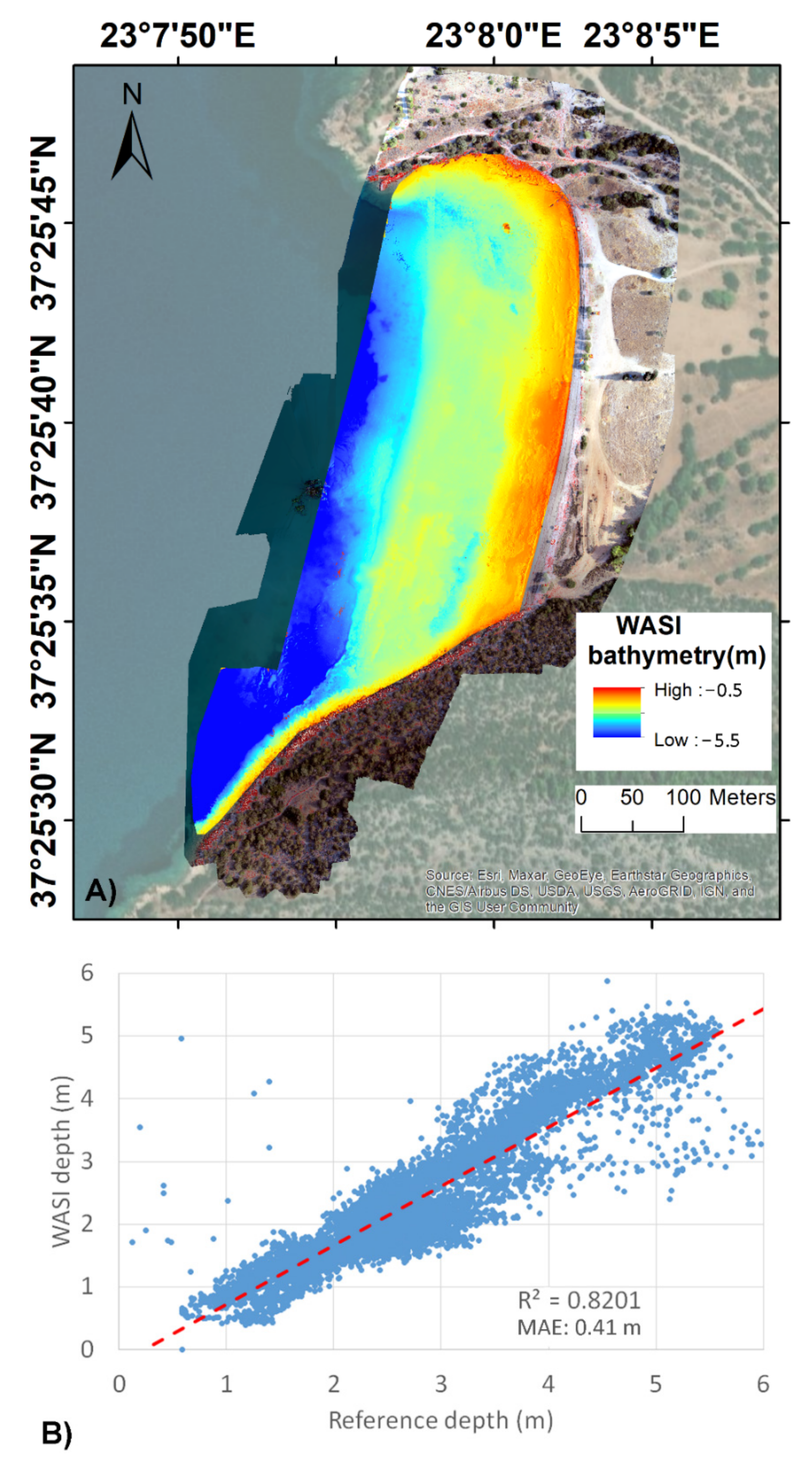
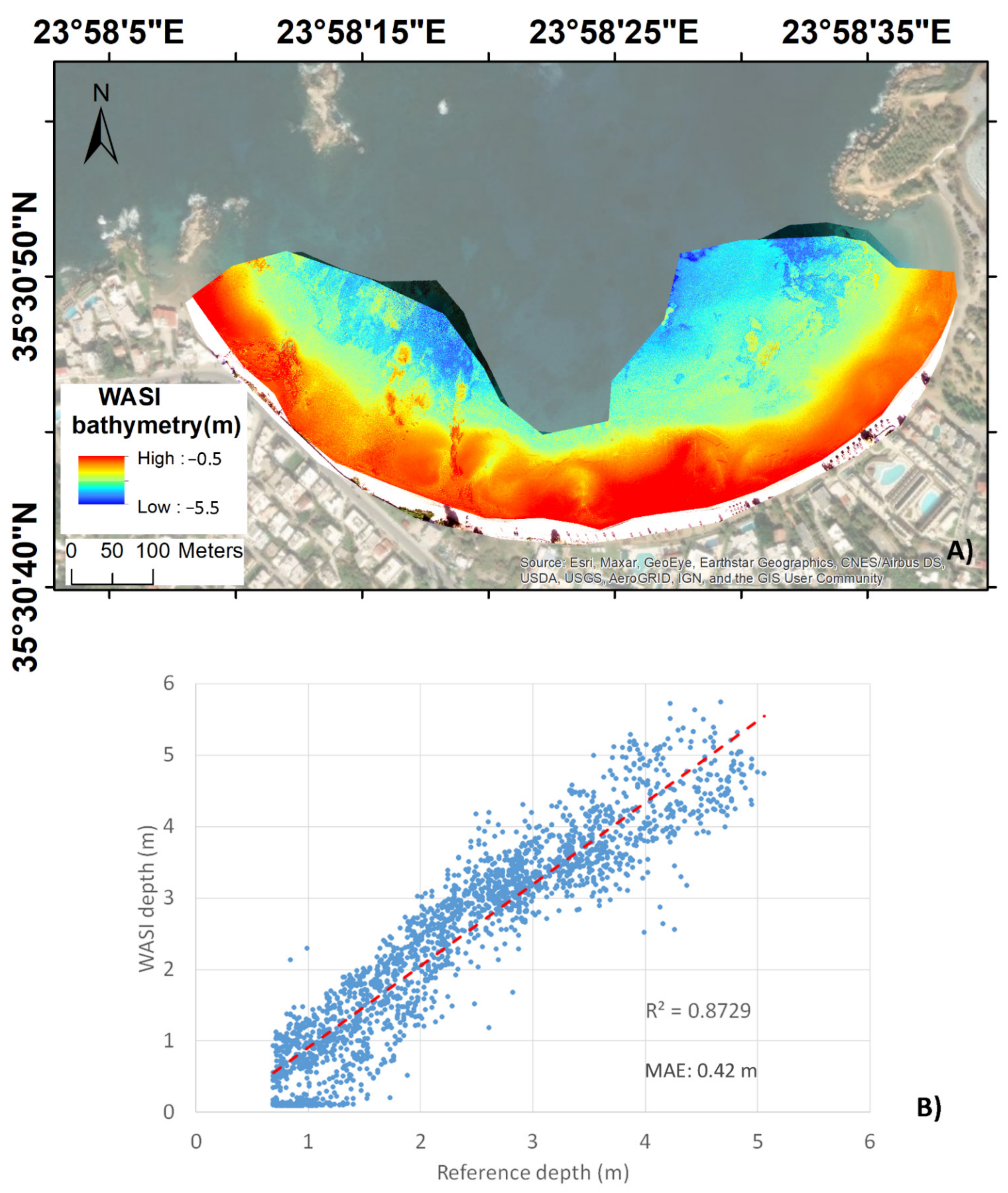
The WASI software is one of the few open-source tools for analyzing the spectral properties of aquatic environments. The WASI tool was initially designed for studying the water properties of freshwater environments and it has been applied on a limited number of bathymetry studies, mainly in lake areas so far [52,53,54]. However, this marks the first time that the WASI software was used for analyzing drone-based imagery, and this is considered an additional novelty of the study. The software is based on earlier bio-optical models developed by [46,55,56]. WASI has a 2D module that allows for image analysis on a per-pixel basis [57]. This is particularly useful for analyzing imagery from multi- or hyper-spectral sensors. Regarding bathymetry retrieval, the WASI tool considers the influence of water-column constituents (IOPs) along with combinations of end-member seafloor reflectance spectra on water-leaving reflectances. For the Lambayanna area, we used one of the default end-member spectra embedded in WASI (Figure 4B). This is a sand-type spectrum that was measured by [58] at shallow depth (0.5 m) using a submersible RAMSES spectroradiometer on the coast of Bolivar (South Australia). The selection of this spectrum was based on in situ observations of the seafloor with snorkeling.
At the study areas of Kalamaki and Plakias, we considered to replace some default end-member spectra of WASI with more appropriate ones that are similar to the seafloor types that were observed during in situ visual assessments along the coastline. Thus, we imported the end-member spectra shown in Figure 4B which include rock, turf algae and brown algae collected underwater with a spectroradiometer and a reference reflectance panel at various coastal locations in the southwest Indian Ocean [49]. Similar end-member spectra collected at different locations show little spectral difference according to [12]; therefore, we considered the above end-member spectra based on their correspondence with in situ observations.
Suitable initial values of geometric (i.e., sun zenith angle) and irradiance model parameters (Table A1, Appendix A) are required for accurate fitting of the spectral signatures. The values of initial model parameters (e.g., chlorophyll-a [CHL-a]; suspended particulate matter [SPM]) were inserted empirically, and their fine-tuning was estimated by fitting a few (2–3) single pixels with known depth. Ideally, in situ water column data should be applied for tuning these parameters; however, collecting such data was not practical in this study. Once the model is tuned, the depth and seafloor type are fitted using the least-squares method iteratively. The modeled spectral signature showing the lowest residual with the observed signature is used to determine the depth and seafloor type for each pixel. A detailed description of the WASI tool can be found in [57].
The remote sensing reflectance in WASI is modeled according to the equations of [46,55]:
R r s s h λ = R r s d e e p λ 1 A r s , 1 exp K d λ + K u W λ Z b + A r s , 2 R r s b λ exp K d λ + K u B λ Z b
The superscript sh indicates shallow water, deep—deep water, b—bottom, and the symbol λ indicates the wavelength. The first term on the right-hand side is the contribution of the water column with depth Zb, the second term represents the contribution of the bottom albedo. Light attenuation is described by the attenuation coefficients Kd for down-welling irradiance, KuW for upwelling radiance originating from the water layer, and KuB for upwelling radiance from the bottom surface. These three coefficients are calculated as a function of the sun zenith angle, viewing direction and the concentrations of water constituents using equations also derived by [46,55]. Ars,1 and Ars,2 are empirical constants.
The WASI algorithm iterates the spectral signatures on a per-pixel basis, trying to fit an optimal spectrum given the constant values of model parameters (Table A2, Appendix A). Inverse modeling takes place by approximating the remote sensing reflectance (Rrs) spectra (of each pixel) with suitable WASI spectra for different depths. The best fit with the observed image spectrum is obtained by minimizing a cost function that calculates the correlation between the Rrs and the WASI spectra. The inversion algorithm employs the absolute difference function in order to identify an optimal set of fit parameters (depth and seafloor type), which minimize the residual of the cost function [54,56,57].

3. Results

The drone-based bathymetry at Lambayanna area (Figure 5A) depicts an overall smooth seafloor with occasional outcrop features, possibly corresponding to beach rock. Bathymetry outputs resulting from shallow water inversion in WASI were validated by fitting a linear regression with in situ sonar measurements (Figure 1 and Figure 2B). At the Lambayanna area, the WASI inverted depths show a very good coefficient of determination with sonar data (R2 = 0.82) and have an MAE of 0.41 m (Figure 5B) and an RMSE of 0.59 m. Lin’s concordance correlation coefficient (LCCC) is 0.85, suggesting that the inversion depths fit well with the sonar measurements. Considering the overall homogeneity of the study area, only one end-member spectrum (WASI sand) was used for inversion within the range of 400–700 nm. The maximum depth estimated by inversion is −5.5 m.
The drone-based bathymetry at Kalamaki bay (Figure 6B) captures fine-scale nearshore bedforms similar to those reported by [10] in this area. The resulting bathymetry fits very well (R2 = 0.87) with USV sonar measurements and has an MAE of 0.42 m and an RMSE of 0.52 m. The LCCC is 0.91, suggesting that inversion depths are in optimal agreement with the sonar measurements. The end-member spectra of WASI-sand, turf algae and brown algae were selected as more suitable for driving the bathymetry inversion in this area, since they correspond with the seafloor cover composition at the Kalamaki area. Inversion took place at the range of 420–600 nm since the pixel values of the MS-red band (660 nm) were too high for the very shallow part (>−1 m) and they were not providing useful reflectance values for deeper (<−2 m) water. The regression plot in Figure 6B shows that there is not an apparent increase in error with increasing depth. The maximum depth estimated by inversion is −5.5 m.
The drone-based bathymetry at Plakias bay (Figure 7A) delineates rocky outcrops and even boulders with sufficient detail. The bathymetry inversion results for the Plakias area (Figure 7B) show a good coefficient of determination (R2 = 0.75) with USV sonar measurements and have an MAE of 0.44 m and an RMSE of 0.58 m. The LCCC is 0.83, suggesting that inversion depths are in good agreement with the sonar measurements. The bathymetry error appears evenly distributed across all depths. Here, three end-member spectra (rock, brown and turf algae) applied for inversion since these two are more prominent in the study area. Inversion took place at the range of 420–600 nm since the pixel values of the MS-red band (660 nm) were too high for the very shallow part (>−1 m) and they were not providing useful reflectance values for deeper (<−2 m) water. The maximum depth estimated by inversion is −7.5 m. Analysis of the bathymetry residuals (absolute difference between reference depth and inverted depth) shows that residuals with large difference values (>2 m) are clearly associated with extremely low reflectance values of the respective bands (Figure 8D,F and Figure 9). Particularly, the pixels corresponding with >2 m depth residuals show the lowest reflectance values in both blue and green bands (for both RGB and MS sensors). Such low reflectance pixels probably represent shaded seafloor or seagrass areas (Figure 8D,F).

4. Discussion

This experimental approach was based on leveraging open-software and literature data (spectra) for producing the first-of-its-kind shallow water bathymetry inversion. The results of this study highlight the effectiveness of hybrid multiband composites for proximal sensing of shallow water bathymetry. Optimal bathymetry results were obtained for all three study areas regardless of the optical complexity of the seafloor types.
The combination of RGB and MS imagery provides a cube with improved spectral resolution in the visible spectrum which is suitable for shallow water inversion. The number of spectral bands determines the detail (and hence the accuracy) at which the seafloor reflectance is approximated and assists in estimating the IOPs values. In addition, only bands sensitive to visible wavelengths are suitable for bathymetry inversion since those are transmitted (some more than others) through the water column without being absorbed or scattered. Particularly, the blue and green wavelengths penetrate deeper into the water column compared to yellow and red wavelengths that are easily absorbed by the first 1–2 m of water depth [28,59]. Our findings suggest that any combination of dual sensors (either RGB or MS) with complementary bands in the visible spectrum are suitable for shallow bathymetry inversion, provided that they are radiometrically calibrated. The overall bathymetric accuracy is <10% of water depth, which is comparable with that from earlier studies using empirical algorithms [31,33].
Drone acquisition during clear, sunny conditions with a calm sea-state provided optimal conditions for capturing representative Rrs values of shallow seafloor and minimized unwanted reflections from the sea surface. Additionally, the close range of the drone to the seafloor assisted in capturing Rrs without the need for applying atmospheric corrections on drone imagery. Drone-based imagery with Rrs values, is required for analyzing imagery with shallow water inversion techniques. Furthermore, end-member spectra are a very important input in shallow bathymetry inversion [53,60]. In the case of Kalamaki beach, it seems that although deeper (>−2 m) parts of the scene are covered with brown algae, bathymetry error is not increasing significantly over those areas (Figure 8C,E). This highlights the robustness of the input end-member spectra for inferring bathymetry in this area. Thus, it is hypothesized that there is a considerable shape similarity between end-member spectra used from the literature and those naturally occurring in the Kalamaki area. At the Lambayanna area, only one end-member spectrum (WASI sand) was sufficient for yielding bathymetry results with low error. This is attributed to the overall homogeneity of the seafloor type in this area. In contrast, at the Plakias area, we applied three end-member spectra in order to better approximate the seafloor types occurring in this complex area.
It is suggested that smooth seafloor geometry at the Lambayanna and Kalamaki areas assisted in calculating more accurate bathymetry inversion than the Plakias area. Smooth seafloor provides a more unobstructed and uniform transmission of seafloor albedo resulting in capturing a clear reflectance signal by drone-based imagery. However, the time-difference between the sonar measurements and the drone survey at Lambayanna area has contributed errors at intermediate depths in the southern part of the area (Figure 8B). This is highlighted further on the plot of Figure 8A where there is a second peak around 0.9 m regarding the frequency of residuals at Lambayanna area. The rugged seafloor surface at Plakias is probably responsible for the observed deviations in bathymetry results. In order to examine this hypothesis, we classified the bathymetry residuals at the Plakias area according to their magnitude and we extracted their corresponding reflectance values for each band. The reflectance boxplots for each residual class and for all bands are shown in Figure 9. These plots reveal that residuals with maximum deviation from actual depth are associated with extremely low reflectance values across all bands of the cube. Consequently, it is inferred that seafloor rugosity is related to cracks and crevices that block sunlight and cast shadows in places, causing significantly lower reflectance values than their surroundings. These obscured areas result in considerable overestimation of depth by the inversion model which falsely fits them with spectral signatures corresponding to deeper waters (Figure 8D,F).
In addition, the results at the Plakias area showed increased errors over seagrass patches (isolated blue spots in Figure 7A and Figure 8D,F) and therefore were not included in the scatterplot in Figure 7B. This issue was encountered even when a seagrass end-member was used in the model. The reason for this problem may be the fact that the characteristic seagrass spectrum beyond the 650 nm range becomes rapidly absorbed even from one-meter depth, leading to confusion with other spectra (e.g., rocks) corresponding to deeper water. Considering that in Plakias bay, seagrass patches occur in areas with at least 2 m depth, it is understood that absorption of red wavelengths in the water column leads to depth overestimation.
This model behavior can be explained by the effect of “non-uniqueness”, which is a common issue hindering bathymetry retrieval from hyperspectral data. This problem has been described by [26,61,62] and is related to the natural phenomenon where different combinations of (a) optically active constituents in the water-column and/or (b) seafloor albedos, can produce the same spectral signature, challenging the accuracy of the final SDB results. In the case of the Plakias area, the seagrass patches are fitted with very deep-water signatures because they cannot be differentiated from the rest of the seafloor types as their spectral features beyond 650 nm are absorbed.
Shallow bathymetry analytical models require careful tuning of initial parameters in order to produce accurate results. By selecting a smaller number of suitable parameters, the model is better constrained and requires less computational resources [54,57]. Thus, when additional information is known (e.g., depth) for a particular location on the image, then model inversion should be applied on individual pixels first, in order to determine the initial values of model parameters (Table A2, Appendix A). Ideally, spectral measurements from a deep water area (where seafloor albedo is negligible) should be collected in order to provide more realistic initial values for CHL-a and SPM [54]. Alternatively, these data could be extracted either from coarse resolution satellite imagery, in situ optical measurements in the water column or from the available literature.

5. Conclusions

This study shows that the integration of drone-based RGB and multispectral imagery provides promising results in shallow bathymetry inversion. Both imagery types are required to be radiometrically corrected and to have complementary bandwidths in the visible range of the spectrum. The multi-band composite cube provides a potentially affordable alternative to costly hyperspectral commercial sensors, allowing for a wider field of shallow water applications. In addition, the cube is suitable for analysis with physics-based optical models, reducing further the costs for obtaining in situ bathymetry data for model calibration. Suitable end-member spectra of local seafloor types should be carefully selected as inputs to shallow analytical algorithms for maximizing the quality of bathymetry output. The presented approach works well across various water types and for relatively smooth seafloor, while seafloor roughness was found to contribute larger bathymetric errors. This novel method is appropriate for high-resolution bathymetry mapping at a landscape scale when only drone imagery is available from areas with sufficient water transparency.

Author Contributions

Conceptualization, E.A.; methodology, E.A.; software, E.A.; validation, E.A.; formal analysis, E.A.; investigation, E.A.; resources, D.D.A.; data curation, D.O. and A.V.A.; writing—original draft preparation, E.A.; writing—review and editing, E.A. and D.D.A.; visualization, E.A.; supervision, E.A. and D.D.A.; project administration, E.A. and D.D.A.; funding acquisition, E.A. and D.D.A. All authors have read and agreed to the published version of the manuscript.

Funding

This research was funded by a 2020 FORTH-Synergy Grant.

Data Availability Statement

Data are available on request from the authors.

Acknowledgments

This study is part of the ACTYS project (https://actys.ims.forth.gr/), (Rethymno, Greece). We would like to thank the anonymous reviewers of this paper for their constructive feedback. In addition, we would like to thank Peter Gege for providing valuable feedback regarding the WASI software.

Conflicts of Interest

The authors declare no conflict of interest.

Appendix A

Table A1. Spectral information included in the header file of each cube. * full-width at half maximum.
Band NameCentral Wavelength (nm)Fwhm* (nm)
P4P-Blue46240
P4P-Green52550
P4P-Red59225
MS-Blue48010
MS-Green56010
MS-Red6715
Table A2. Values of water IOPs used as constants in this study.
Study AreaCHL-a (mg/L)SPM (mg/L)
Lambayanna0.30.3
Kalamaki0.180.13
Plakias0.180.10

References

  1. Bio, A.; Bastos, L.; Granja, H.; Pinho, J.L.S.; Gonçalves, J.A.; Henriques, R.; Madeira, S.; Magalhães, A.; Rodrigues, D. Methods for Coastal Monitoring and Erosion Risk Assessment: Two Portuguese Case Studies. RGCI 2015, 15, 47–63. [Google Scholar] [CrossRef] [Green Version]
  2. Davidson, M.; Van Koningsveld, M.; de Kruif, A.; Rawson, J.; Holman, R.; Lamberti, A.; Medina, R.; Kroon, A.; Aarninkhof, S. The CoastView Project: Developing Video-Derived Coastal State Indicators in Support of Coastal Zone Management. Coast. Eng. 2007, 54, 463–475. [Google Scholar] [CrossRef]
  3. Deronde, B.; Houthuys, R.; Debruyn, W.; Fransaer, D.; Lancker, V.V.; Henriet, J.-P. Use of Airborne Hyperspectral Data and Laserscan Data to Study Beach Morphodynamics along the Belgian Coast. Coas 2006, 2006, 1108–1117. [Google Scholar] [CrossRef]
  4. Papadopoulos, N.; Oikonomou, D.; Cantoro, G.; Simyrdanis, K.; Beck, J. Archaeological Prospection in Ultra-Shallow Aquatic Environments: The Case of the Prehistoric Submerged Site of Lambayanna, Greece. Near Surf. Geophys. 2021, 19, 677–697. [Google Scholar] [CrossRef]
  5. Wiseman, C.; O’Leary, M.; Hacker, J.; Stankiewicz, F.; McCarthy, J.; Beckett, E.; Leach, J.; Baggaley, P.; Collins, C.; Ulm, S.; et al. A Multi-Scalar Approach to Marine Survey and Underwater Archaeological Site Prospection in Murujuga, Western Australia. Quat. Int. 2021, 584, 152–170. [Google Scholar] [CrossRef]
  6. Costa, B.M.; Battista, T.A.; Pittman, S.J. Comparative Evaluation of Airborne LiDAR and Ship-Based Multibeam SoNAR Bathymetry and Intensity for Mapping Coral Reef Ecosystems. Remote Sens. Environ. 2009, 113, 1082–1100. [Google Scholar] [CrossRef]
  7. Goes, E.R.; Brown, C.J.; Araújo, T.C. Geomorphological Classification of the Benthic Structures on a Tropical Continental Shelf. Front. Mar. Sci. 2019, 6, 47. [Google Scholar] [CrossRef]
  8. Zhang, C. Applying Data Fusion Techniques for Benthic Habitat Mapping and Monitoring in a Coral Reef Ecosystem. ISPRS J. Photogramm. Remote Sens. 2015, 104, 213–223. [Google Scholar] [CrossRef]
  9. Carvalho, R.C.; Hamylton, S.; Woodroffe, C.D. Filling the ‘White Ribbon’ in Temperate Australia: A Multi-Approach Method to Map the Terrestrial-Marine Interface. In Proceedings of the 2017 IEEE/OES Acoustics in Underwater Geosciences Symposium (RIO Acoustics), Rio de Janeiro, Brazil, 25–27 July 2017; pp. 1–5. [Google Scholar]
  10. Alevizos, E.; Roussos, A.; Alexakis, D. Geomorphometric Analysis of Nearshore Sedimentary Bedforms from High-Resolution Multi-Temporal Satellite-Derived Bathymetry. Geocarto Int. 2021, 1–17. [Google Scholar] [CrossRef]
  11. Kenny, A.J.; Cato, I.; Desprez, M.; Fader, G.; Schüttenhelm, R.T.E.; Side, J. An Overview of Seabed-Mapping Technologies in the Context of Marine Habitat Classification. ICES J. Mar. Sci. 2003, 60, 411–418. [Google Scholar] [CrossRef] [Green Version]
  12. Kutser, T.; Hedley, J.; Giardino, C.; Roelfsema, C.; Brando, V.E. Remote Sensing of Shallow Waters—A 50 Year Retrospective and Future Directions. Remote Sens. Environ. 2020, 240, 111619. [Google Scholar] [CrossRef]
  13. Lyzenga, D.R. Passive Remote Sensing Techniques for Mapping Water Depth and Bottom Features. Appl. Opt. 1978, 17, 379–383. [Google Scholar] [CrossRef] [PubMed]
  14. Stumpf, R.P.; Holderied, K.; Sinclair, M. Determination of Water Depth with High-Resolution Satellite Imagery over Variable Bottom Types. Limnol. Oceanogr. 2003, 48, 547–556. [Google Scholar] [CrossRef]
  15. Geyman, E.C.; Maloof, A.C. A Simple Method for Extracting Water Depth From Multispectral Satellite Imagery in Regions of Variable Bottom Type. Earth Space Sci. 2019, 6, 527–537. [Google Scholar] [CrossRef]
  16. Gholamalifard, M.; Kutser, T.; Esmaili-Sari, A.; Abkar, A.A.; Naimi, B. Remotely Sensed Empirical Modeling of Bathymetry in the Southeastern Caspian Sea. Remote Sens. 2013, 5, 2746–2762. [Google Scholar] [CrossRef] [Green Version]
  17. Ma, S.; Tao, Z.; Yang, X.; Yu, Y.; Zhou, X.; Li, Z. Bathymetry Retrieval From Hyperspectral Remote Sensing Data in Optical-Shallow Water. IEEE Trans. Geosci. Remote Sens. 2014, 52, 1205–1212. [Google Scholar] [CrossRef]
  18. Traganos, D.; Poursanidis, D.; Aggarwal, B.; Chrysoulakis, N.; Reinartz, P. Estimating Satellite-Derived Bathymetry (SDB) with the Google Earth Engine and Sentinel-2. Remote Sens. 2018, 10, 859. [Google Scholar] [CrossRef] [Green Version]
  19. Wei, C.; Zhao, Q.; Lu, Y.; Fu, D. Assessment of Empirical Algorithms for Shallow Water Bathymetry Using Multi-Spectral Imagery of Pearl River Delta Coast, China. Remote Sens. 2021, 13, 3123. [Google Scholar] [CrossRef]
  20. Kibele, J.; Shears, N.T. Nonparametric Empirical Depth Regression for Bathymetric Mapping in Coastal Waters. IEEE J. Sel. Top. Appl. Earth Obs. Remote Sens. 2016, 9, 5130–5138. [Google Scholar] [CrossRef]
  21. Caballero, I.; Stumpf, R.P. Retrieval of Nearshore Bathymetry from Sentinel-2A and 2B Satellites in South Florida Coastal Waters. Estuar. Coast. Shelf Sci. 2019, 226, 106277. [Google Scholar] [CrossRef]
  22. Dekker, A.G.; Phinn, S.R.; Anstee, J.; Bissett, P.; Brando, V.E.; Casey, B.; Fearns, P.; Hedley, J.; Klonowski, W.; Lee, Z.P.; et al. Intercomparison of Shallow Water Bathymetry, Hydro-Optics, and Benthos Mapping Techniques in Australian and Caribbean Coastal Environments. Limnol. Oceanogr. Methods 2011, 9, 396–425. [Google Scholar] [CrossRef] [Green Version]
  23. Klonowski, W.M. Retrieving Key Benthic Cover Types and Bathymetry from Hyperspectral Imagery. J. Appl. Remote Sens. 2007, 1, 011505. [Google Scholar] [CrossRef]
  24. Leiper, I.A.; Phinn, S.R.; Roelfsema, C.M.; Joyce, K.E.; Dekker, A.G. Mapping Coral Reef Benthos, Substrates, and Bathymetry, Using Compact Airborne Spectrographic Imager (CASI) Data. Remote Sens. 2014, 6, 6423–6445. [Google Scholar] [CrossRef] [Green Version]
  25. Lee, Z.; Carder, K.L.; Mobley, C.D.; Steward, R.G.; Patch, J.S. Hyperspectral Remote Sensing for Shallow Waters: 2. Deriving Bottom Depths and Water Properties by Optimization. Appl. Opt. 1999, 38, 3831–3843. [Google Scholar] [CrossRef] [Green Version]
  26. Mobley, C.D.; Sundman, L.K.; Davis, C.O.; Bowles, J.H.; Downes, T.V.; Leathers, R.A.; Montes, M.J.; Bissett, W.P.; Kohler, D.D.R.; Reid, R.P.; et al. Interpretation of Hyperspectral Remote-Sensing Imagery by Spectrum Matching and Look-up Tables. Appl. Opt. 2005, 44, 3576–3592. [Google Scholar] [CrossRef]
  27. Castillo-López, E.; Dominguez, J.A.; Pereda, R.; de Luis, J.M.; Pérez, R.; Piña, F. The Importance of Atmospheric Correction for Airborne Hyperspectral Remote Sensing of Shallow Waters: Application to Depth Estimation. Atmos. Meas. Tech. 2017, 10, 3919–3929. [Google Scholar] [CrossRef] [Green Version]
  28. Kobryn, H.T.; Wouters, K.; Beckley, L.E.; Heege, T. Ningaloo Reef: Shallow Marine Habitats Mapped Using a Hyperspectral Sensor. PLoS ONE 2013, 8, e70105. [Google Scholar] [CrossRef] [Green Version]
  29. Alevizos, E. How to Create High Resolution Digital Elevation Models of Terrestrial Landscape Using Uav Imagery and Open-Source Software. 2019. Available online: https://www.researchgate.net/publication/333248069_HOW_TO_CREATE_HIGH_RESOLUTION_DIGITAL_ELEVATION_MODELS_OF_TERRESTRIAL_LANDSCAPE_USING_UAV_IMAGERY_AND_OPEN-SOURCE_SOFTWARE (accessed on 1 October 2021).
  30. Román, A.; Tovar-Sánchez, A.; Olivé, I.; Navarro, G. Using a UAV-Mounted Multispectral Camera for the Monitoring of Marine Macrophytes. Front. Mar. Sci. 2021, 8, 722698. [Google Scholar] [CrossRef]
  31. Rossi, L.; Mammi, I.; Pelliccia, F. UAV-Derived Multispectral Bathymetry. Remote Sens. 2020, 12, 3897. [Google Scholar] [CrossRef]
  32. Parsons, M.; Bratanov, D.; Gaston, K.; Gonzalez, F. UAVs, Hyperspectral Remote Sensing, and Machine Learning Revolutionizing Reef Monitoring. Sensors 2018, 18, 2026. [Google Scholar] [CrossRef] [Green Version]
  33. Slocum, R.K.; Parrish, C.E.; Simpson, C.H. Combined Geometric-Radiometric and Neural Network Approach to Shallow Bathymetric Mapping with UAS Imagery. ISPRS J. Photogramm. Remote Sens. 2020, 169, 351–363. [Google Scholar] [CrossRef]
  34. Starek, M.J.; Giessel, J. Fusion of Uas-Based Structure-from-Motion and Optical Inversion for Seamless Topo-Bathymetric Mapping. In Proceedings of the 2017 IEEE International Geoscience and Remote Sensing Symposium (IGARSS), Fort Worth, TX, USA, 23–28 July 2017; pp. 2999–3002. [Google Scholar]
  35. Chirayath, V.; Earle, S.A. Drones That See through Waves–Preliminary Results from Airborne Fluid Lensing for Centimetre-Scale Aquatic Conservation. Aquat. Conserv. Mar. Freshw. Ecosyst. 2016, 26, 237–250. [Google Scholar] [CrossRef] [Green Version]
  36. Manfreda, S.; McCabe, M.F.; Miller, P.E.; Lucas, R.; Pajuelo Madrigal, V.; Mallinis, G.; Ben Dor, E.; Helman, D.; Estes, L.; Ciraolo, G.; et al. On the Use of Unmanned Aerial Systems for Environmental Monitoring. Remote Sens. 2018, 10, 641. [Google Scholar] [CrossRef] [Green Version]
  37. Isgró, M.A.; Basallote, M.D.; Barbero, L. Unmanned Aerial System-Based Multispectral Water Quality Monitoring in the Iberian Pyrite Belt (SW Spain). Mine Water Environ. 2021. [Google Scholar] [CrossRef]
  38. Kabiri, K.; Rezai, H.; Moradi, M. A Drone-Based Method for Mapping the Coral Reefs in the Shallow Coastal Waters – Case Study: Kish Island, Persian Gulf. Earth Sci. Inform. 2020, 13, 1265–1274. [Google Scholar] [CrossRef]
  39. Fallati, L.; Saponari, L.; Savini, A.; Marchese, F.; Corselli, C.; Galli, P. Multi-Temporal UAV Data and Object-Based Image Analysis (OBIA) for Estimation of Substrate Changes in a Post-Bleaching Scenario on a Maldivian Reef. Remote Sens. 2020, 12, 2093. [Google Scholar] [CrossRef]
  40. Murfitt, S.L.; Allan, B.M.; Bellgrove, A.; Rattray, A.; Young, M.A.; Ierodiaconou, D. Applications of Unmanned Aerial Vehicles in Intertidal Reef Monitoring. Sci. Rep. 2017, 7, 10259. [Google Scholar] [CrossRef] [Green Version]
  41. Rossiter, T.; Furey, T.; McCarthy, T.; Stengel, D.B. UAV-Mounted Hyperspectral Mapping of Intertidal Macroalgae. Estuar. Coast. Shelf Sci. 2020, 242, 106789. [Google Scholar] [CrossRef]
  42. Tait, L.; Bind, J.; Charan-Dixon, H.; Hawes, I.; Pirker, J.; Schiel, D. Unmanned Aerial Vehicles (UAVs) for Monitoring Macroalgal Biodiversity: Comparison of RGB and Multispectral Imaging Sensors for Biodiversity Assessments. Remote Sens. 2019, 11, 2332. [Google Scholar] [CrossRef] [Green Version]
  43. Barnhart, H.X.; Haber, M.; Song, J. Overall Concordance Correlation Coefficient for Evaluating Agreement among Multiple Observers. Biometrics 2002, 58, 1020–1027. [Google Scholar] [CrossRef]
  44. Lin, L.; Hedayat, A.S.; Wu, W. A Unified Approach for Assessing Agreement for Continuous and Categorical Data. J. Biopharm. Stat. 2007, 17, 629–652. [Google Scholar] [CrossRef] [PubMed]
  45. Zhao, D.; Arshad, M.; Wang, J.; Triantafilis, J. Soil Exchangeable Cations Estimation Using Vis-NIR Spectroscopy in Different Depths: Effects of Multiple Calibration Models and Spiking. Comput. Electron. Agric. 2021, 182, 105990. [Google Scholar] [CrossRef]
  46. Albert, A. Inversion Technique for Optical Remote Sensing in Shallow Water. Ph.D. Thesis, Hamburg University, Hamburg, Germany, December 2004. Available online: https://ediss.sub.unihamburg.de/handle/ediss/812 (accessed on 1 October 2021).
  47. Tagle, X. Study of Radiometric Variations in Unmanned Aerial Vehicle Remote Sensing Imagery for Vegetation Mapping. Master’s Thesis, Lund University, Lund, Sweden, June 2017. [Google Scholar] [CrossRef]
  48. Burggraaff, O.; Schmidt, N.; Zamorano, J.; Pauly, K.; Pascual, S.; Tapia, C.; Spyrakos, E.; Snik, F. Standardized Spectral and Radiometric Calibration of Consumer Cameras. Opt. Express 2019, 27, 19075. [Google Scholar] [CrossRef] [PubMed] [Green Version]
  49. Mouquet, P.; Quod, J.-P. Spectrhabent-OI-Acquisition et Analyse de la Librairie Spectrale Sous-Marine. 2010. Available online: https://archimer.ifremer.fr/doc/00005/11647/ (accessed on 1 October 2021).
  50. Alevizos, E.; Alexakis, D.D. Evaluation of Radiometric Calibration of Drone-Based Imagery for Improving Shallow Bathymetry Retrieval. Remote Sens. Lett. 2022, 13, 311–321. [Google Scholar] [CrossRef]
  51. Radiometric Calibration Model for MicaSense Sensors. Available online: https://support.micasense.com/hc/en-us/articles/115000351194-Radiometric-Calibration-Model-for-MicaSense-Sensors (accessed on 23 October 2021).
  52. Gege, P. A Case Study at Starnberger See for Hyperspectral Bathymetry Mapping Using Inverse Modeling. In Proceedings of the 2014 6th Workshop on Hyperspectral Image and Signal Processing: Evolution in Remote Sensing (WHISPERS), Lausanne, Switzerland, 24–27 June 2014; pp. 1–4. [Google Scholar]
  53. Dörnhöfer, K.; Göritz, A.; Gege, P.; Pflug, B.; Oppelt, N. Water Constituents and Water Depth Retrieval from Sentinel-2A—A First Evaluation in an Oligotrophic Lake. Remote Sens. 2016, 8, 941. [Google Scholar] [CrossRef] [Green Version]
  54. Niroumand-Jadidi, M.; Bovolo, F.; Bruzzone, L.; Gege, P. Physics-Based Bathymetry and Water Quality Retrieval Using PlanetScope Imagery: Impacts of 2020 COVID-19 Lockdown and 2019 Extreme Flood in the Venice Lagoon. Remote Sens. 2020, 12, 2381. [Google Scholar] [CrossRef]
  55. Albert, A.; Mobley, C.D. An Analytical Model for Subsurface Irradiance and Remote Sensing Reflectance in Deep and Shallow Case-2 Waters. Opt. Express 2003, 11, 2873–2890. [Google Scholar] [CrossRef]
  56. Gege, P.; Albert, A. A tool for inverse modeling of spectral measurements in deep and shallow waters. In Remote Sensing of Aquatic Coastal Ecosystem Processes; Richardson, L.L., Ledrew, E.F., Eds.; Remote Sensing and Digital Image Processing; Springer Netherlands: Dordrecht, The Netherlands, 2006; pp. 81–109. ISBN 978-1-4020-3968-3. [Google Scholar]
  57. Gege, P. WASI-2D: A Software Tool for Regionally Optimized Analysis of Imaging Spectrometer Data from Deep and Shallow Waters. Comput. Geosci. 2014, 62, 208–215. [Google Scholar] [CrossRef] [Green Version]
  58. Pinnel, N. A method for mapping submerged macrophytes in lakes using hyperspectral remote sensing. Ph.D. Thesis, Technischen Universitaet Muenchen, München, Germany, 2007. Available online: https://mediatum.ub.tum.de/doc/604557/document.pdf (accessed on 5 November 2021).
  59. Eugenio, F.; Marcello, J.; Martin, J.; Rodríguez-Esparragón, D. Benthic Habitat Mapping Using Multispectral High-Resolution Imagery: Evaluation of Shallow Water Atmospheric Correction Techniques. Sensors 2017, 17, 2639. [Google Scholar] [CrossRef] [Green Version]
  60. Garcia, R.A.; Lee, Z.; Hochberg, E.J. Hyperspectral Shallow-Water Remote Sensing with an Enhanced Benthic Classifier. Remote Sens. 2018, 10, 147. [Google Scholar] [CrossRef] [Green Version]
  61. Defoin-Platel, M.; Chami, M. How Ambiguous Is the Inverse Problem of Ocean Color in Coastal Waters? J. Geophys. Res. Ocean. 2007, 112. [Google Scholar] [CrossRef] [Green Version]
  62. Garcia, R.A. Uncertainty in Hyperspectral Remote Sensing: Analysis of the Potential and Limitation of Shallow Water Bathymetry and Benthic Classification. Ph.D. Thesis, Curtin University, Perth, Australia, October 2015. [Google Scholar]
Figure 1. Overview maps of the study areas overlaid with true color of drone-based mosaics. (A) Map legend (Greece); (B) Lambayanna area; (C) Kalamaki area; (D) Plakias area. Red lines indicate the USV tracks. (At Lambayanna, the whole area was covered with dense tracks of the inflatable boat and thus these are not presented for visualization purposes).
Remotesensing 14 01127 g001
Figure 2. (A) Schematic representation of the USV platform and sensors deployed at Kalamaki and Plakias areas; (B) Boxplots of the sonar depth measurements collected at each area. The black horizontal line inside each box indicates the median value of each sample, and the numbers at the horizontal axis indicate the number of measurements in each area.
Remotesensing 14 01127 g002
Figure 3. Workflow diagram of the methodology followed in this study.
Remotesensing 14 01127 g003
Figure 4. (A) Spectral responses of both P4P and MS sensors (modified from [47,48]); (B) End-member spectra used for inversion in WASI (from [49]).
Remotesensing 14 01127 g004
Figure 5. (A) Lambayanna area bathymetry resulting from inversion of the 6-band composite in WASI; (B) Linear regression plot between the WASI bathymetry and sonar-based measurements.
Remotesensing 14 01127 g005
Figure 6. (A) Kalamaki area bathymetry resulting from inversion of the 6-band composite in WASI; (B) Linear regression plot between the WASI bathymetry and USV sonar-based measurements.
Remotesensing 14 01127 g006
Figure 7. (A) Plakias area bathymetry resulting from inversion of the 6-band composite in WASI, and isolated spots with blue color in the middle of the map correspond to errors over seagrass patches; (B) Linear regression plot between the WASI bathymetry and USV sonar-based measurements.
Remotesensing 14 01127 g007
Figure 8. (A) Frequency distribution plot of the residual bathymetric error at each area. Comparison between sonar and inversion bathymetric profiles overlaid with true-color mosaic stripes for the (B) Lambayanna area, (C,E) Kalamaki area and (D,F) Plakias area.
Remotesensing 14 01127 g008
Figure 9. Boxplots showing the correspondence between different depth residual classes and RGB-MS reflectance values for the Plakias area.
Remotesensing 14 01127 g009
Table 1. Drone survey details for each study area.
Study AreaNumber of RGB ImagesNumber of MS ImagesAltitudeSun Zenith Angle (Degrees)Acquisition Time (hh:mm)
Lambayanna beach500>1000907009:00
Kalamaki bay4004001505211:30
Plakias bay2302001504912:00
Publisher’s Note: MDPI stays neutral with regard to jurisdictional claims in published maps and institutional affiliations.

