Alien Pulse Rejection in Concurrent Firing LIDAR

Abstract

Mobile pulse light detection and ranging (LIDAR) is an essential component of autonomous vehicles. The obstacle detection function of autonomous vehicles requires very low failure rates. With an increasing number of autonomous vehicles equipped with LIDAR sensors for use in the detection and avoidance of obstacles and for safe navigation through the environment, the probability of mutual interference becomes an important issue. The reception of foreign laser pulses can lead to problems such as ghost targets or a reduced signal-to-noise ratio (SNR). In this paper, we presented the probability that any LIDAR sensor would interfere mutually by considering spatial and temporal overlaps. We presented some typical mutual interference scenarios in real-world vehicle applications, as well as an analysis of the interference mechanism. We proposed a new multi-plane LIDAR sensor which used coded pulse streams encoded by carrier-hopping prime code (CHPC) technology to measure surrounding perimeters without mutual interference. These encoded pulses utilized a random azimuth identification and checksum with random spreading code. We modeled the entirety of the LIDAR sensor operation in Synopsys OptSim and represented the alien pulse elimination functionality obtained via modeling and simulation.

1. Introduction

Range sensors are devices that capture the three-dimensional (3-D) structure of the world from the viewpoint of the sensor, usually measuring distances to closest targets [1,2,3,4,5]. These measurements could be across a scanning plane or a 3-D image with distance measurements at every point.

These range sensors have been used for many years in the fields of localization, obstacle detection and tracking for autonomous vehicles [6,7]. These can be employed as measurement devices to address the joint problem of online tracking and the detection of the current modality [8]. These can be helpful indicators for use in sustainability assessment by presenting the distribution characteristics of each sustainability index for vehicles [9]. Obstacle detection functions of autonomous vehicles require low failure rates [10]. Interference is inherent to all active sensors and wireless applications with the same or an overlapping frequency range [11,12,13,14]. In general, interference describes the coherent superposition of two or more different waves at one point in space. A wave is a rotating vector in the complex plane, where the addition of several vectors results in deterministic changes to magnitude and phase. Signal amplitude can be decreased (destructive interference) or increased (constructive interference). Single interference can be treated as one-shot noise or error and can be eliminated using the Kalman filter or the particle learning technique [15,16].

Within a few years, the adaption rate of vehicular radio detection and ranging (radar) systems will have drastically increased in this newly emerging market [17]. In terms of safety-related applications, interference risk will particularly threaten further proliferation if harmful mutual interference occurs [18,19,20]. It is too late to find efficient and pragmatic countermeasures to avoid apparent interference risk when severe interference problems cause malfunction or out-of-order situations in safety radar devices [14,21]. The only reasonable and valid approach is to counteract these issues before the problems are manifested. The EU funding project, more safety for all by radar interference mitigation (MOSARIM), started in January 2010, intending to investigate possible automotive radar interference mechanisms via both simulation and real-world road tests [18,19,20,22]. Interference from an identical pulsed radar sensor with the same pulse repetition frequency (PRF) generates a ghost target at a constant distance. If the radars are similar, and only have slightly different PRFs, then a ghost target will appear as a large target moving slowly in the range. The apparent velocity is dependent on the difference between the two PRFs and could be anything from a couple of millimeters per second up to a couple of hundred meters per second. A slightly different PRF results in a moving ghost target, as the time difference between the transmitted pulse and the interfering pulse increases or decreases from pulse repetition period to pulse repetition period. If the PRFs are vastly different, then more than one ghost target could appear per cycle [11,23]. Appropriate countermeasures and mitigation techniques were studied and assessed, and general guidelines and recommendations were developed [11,23,24,25]. The ideas for countermeasures were extracted and structured into six basic categories. From the six basic categories, a list of 22 variants was compiled, evaluated, and ranked concerning various criteria for the implementation effort, required power and computational resources, cost, the requirement for harmonization, etc. They selected the top nine countermeasures for further evaluation in order to derive guidelines. Their mitigation performance ranged from a few $\mathrm{dB}$ up to (theoretically) infinite $\mathrm{dB}$. Their accurate and consistent application to all new automotive radar products will result in close to interference-free automotive radar operations.

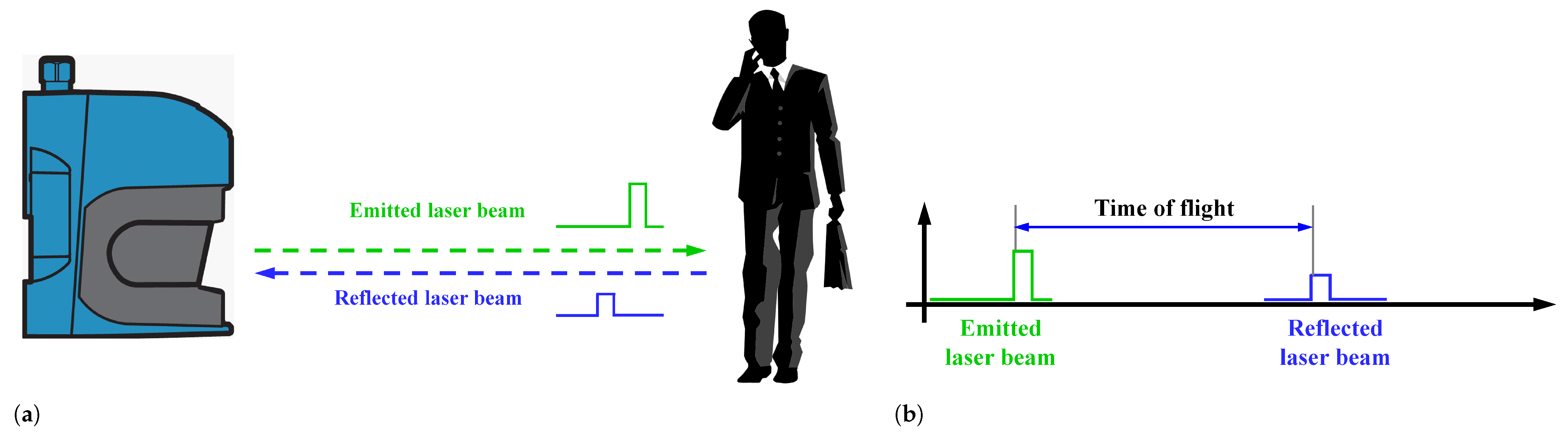
Time-of-flight (ToF) range cameras acquire a 3-D image of a scene simultaneously for all pixels from a single viewing location. Optical interference between a sensor and another sensor is a crucial matter [26]. It is not easy to separate the amplitude-modulated wave from the sensor itself and another sensor once they are mixed. This shows how the mixed pixel and multipath separation algorithm can be applied to range imaging measurements projected into Cartesian coordinates. Significant improvements in accuracy can be achieved in particular situations where the influence of multipath interference frequently causes distortions [27,28,29]. The multiple return separation algorithm requires a consistent and known relationship between the cameras’ amplitudes and phase responses at both modulation frequencies. This type of calibration was not available for these cameras, so it was carried out by comparing manually selected regions of the image judged to be minimally affected by multipath interference. If these regions did contain multipath, the calibration would be compromised, leading to poor performance. Another source of potential error is distance linearity measurement inaccuracies, which are common in uncalibrated range cameras. It is also possible that the optimization algorithm encountered local minima, producing an incorrect answer.

The light detection and ranging (LIDAR) sensor is one of the essential perception sensors for autonomous vehicles that can travel autonomously [1,2,3,4,5,6,7,10]. A LIDAR sensor installed on an autonomous vehicle lets this vehicle generate a detailed 3-D local map of its environment. Histogram analysis of the 3-D local map is used to select the obstacle candidates. It incorporates matched candidates into results from previous scans and updates the positions of all obstacles based on vehicle motion before the following scan. The car then takes these maps and combines them with high-resolution global maps of the world, producing different types of maps that allow it to drive itself. The reception of foreign laser pulses can lead to ghost targets or a reduced signal-to-noise ratio. The reception of unwanted laser pulses from other LIDAR sensors is called mutual interference between LIDAR sensors [30,31,32,33,34,35,36,37]. Concretely, interference effects in automotive LIDAR sensors are caused by the superposition of disturbances from other LIDAR sensors at the receiving antenna with the incoming coherent use signals being reflected from objects within the LIDAR sensor’s detection zone. The simplest method for the prevention of such interference is to install each sensor by tilting them forward 2° to 3°. However, that is not enough. Another measure is to emit as few lasers as possible. The laser should be off where sensor data are unnecessary. According to the analyzed result, the laser was automatically off in unnecessary areas and scans were curtailed. These functions prevent interference and extend laser devices and reduce power consumption. Moreover, one more step is ready for use, which is a function where motor speed is slightly changed on command. A difference in motor speed that is more than 300 almost prevents interference [38].

Until now, interference has not been considered as a problem because the number of vehicles equipped with LIDAR sensors was small, and, as a result, the possibility of interference was extremely unlikely. So, despite a predicted higher number of LIDAR sensors, the possibility of interference-induced problems has to be reduced considerably. With the increase in the number of autonomous vehicles equipped with LIDAR sensors for use in obstacle detection and avoidance for safe navigation through environments, the possibility of mutual interference becomes an issue. Imagine massive traffic jams occurring in the morning and evening. What if all of these vehicles were equipped with LIDAR sensors? With a growing number of autonomous vehicles equipped with LIDAR sensors operating close to each other at the same time, LIDAR sensors may receive laser pulses from other LIDAR sensors.

This article is structured as follows: in Section 2, the occurrence of mutual interference in radar and LIDAR sensors is discussed. The causes of mutual interference and the extensive study of radar sensor interference in the MOSARIM project are briefly described. In Section 3, a new multi-plane LIDAR sensor, which uses coded pulse streams to measure surrounding perimeters without mutual interference, is presented. In Section 4, three relevant mutual interference scenarios in real-world vehicle applications of simulations are presented. In Section 5, four different simulation phases are set up according to the operating mode of two LIDAR sensors, and their results are shown. In each scenario, LIDAR sensors operated in single-pulse mode suffered from mutual interference, but LIDAR sensors with a coded pulse steam mode effectively rejected alien pulses. In Section 6, the conclusion is given, and future research paths are suggested.

2. Occurrence of Mutual Interference

Some studies have been performed regarding the depiction of the occurrence of mutual interference between LIDAR sensors and improvement of the design of pulsed LIDAR sensors. Kim et al. [30,31,32,33] presented two LMS-511 LIDAR sensors that operated simultaneously in a closed space, resulting in mutual interference. Popko et al. [35,36] carried out similar experiments with two LIDAR sensors. In their articles, signal intersections occurring between sensors were analyzed, and based on this, a geometric proximity model for mutual interference was presented. They introduced the terms direct interference and indirect interference. Direct interference occurs when two LIDAR sensors are oriented at each other, and a signal from one is coupled into the other’s receiver. Indirect interference, or scattering interference, occurs when the target scattering of one LIDAR sensor’s signal is received by another. Unlike radar sensors, where direct interference accounts for the majority of cases of interference, indirect interference makes up almost the majority of interferences generated by LIDAR sensors. Hwang et al. [37] investigated the characteristics and impacts of mutual interference with regard to a LIDAR sensor using an analog true-random signal for autonomous vehicle applications. Lo et al. [39] proposed a proof-of -principle LIDAR and demonstrated the superiority of two-dimensional (2-D) LIDAR modulation on interference robustness and the elimination of the near–far effect.

2.1. Direct Time-of-Flight and Mutual Interference

A LIDAR sensor measures the distance to an object on the direct time-of-flight (dToF) principle based on the known speed of light (299,792,458 $\mathrm{m}$ ${\mathrm{s}}^{-1}$) by emitting an object with a laser pulse and analyzing the reflected laser pulse. As illustrated in Figure 1, it transmits a 5 ns to 20 ns laser pulse toward an object and measures the time taken by the laser pulse to be reflected off the object and returned to the sender. The incoming laser pulse causes a delay depending on the distance of the object. The LIDAR sensor calculates that a distance to a target is half the round-trip transit time multiplied by the speed of light.

Furthermore, LIDAR sensors are exposed to various emissions from other users, such as LIDAR sensors in other cars at near distances and other LIDAR sensors roadside or on closed roads. As shown in Figure 2, multiple LIDAR sensors operate in proximity to each other and thus generate mutual interference. If two or more LIDAR sensors that are in proximity to each other transmit pulses in the same operating frequency band, each LIDAR sensor system will receive reflected signals of the other LIDAR sensors. These reflected signals are more or less indistinguishable from reflections from their targets. These received interference signals can be of similar amplitude and can confuse receiving systems and target displays. This well-known problem manifests itself in increases in false alarm rates and in undesirable losses of sensitivity for the detection of targets. Mutual interference is a severe problem for many types of LIDAR sensors and leads to a continuing problem for future LIDAR sensor concepts.

2.2. Relevant Mutual Interference Scenarios in Real-World Vehicle Applications

In order to investigate radar sensor interference in the MOSARIM project, they selected scenarios that were particularly relevant to be considered for analysis in simulation and practical measurements based on the partner’s experience [19]. The scenario selection took into account a number of different factors, apart from obvious direct interference from one radar sensor to another. According to relevant vehicle applications in which radar sensors are typically used to detect surrounding vehicles or objects, they divide these mutual interference scenarios into two main categories: direct interference scenarios as listed in

Table 1. Relevant direct interference traffic scenarios of forward-looking radar sensors without further target objects.

Scenario Name	Main Scenario Factor	Potential Interference Effect
Standstill, short and long distance	Stationary victim vehicle and interferer in direct field of view	Occurrence of ghost targets
Victim approaches interferer	Victim approaches stationary interferer in direct field of view	Occurrence of ghost targets, observation of signal/noise ratio (SNR) while approaching
Victim and interferer pass each other	Radar sensor interferes within each other vehicle’s radar main-lobe	Occurrence of ghost target

,

Table 2. Relevant direct interference traffic scenarios of forward-looking radar sensors with rear- or sideward-looking sensors.

Scenario Name	Main Scenario Factor	Potential Interference Effect
Traffic in same direction with similar velocities, rear sensor	Victim drives on the same lane behind the interfering vehicle	Interference-increased noise may make interfering vehicle invisible
Overtaking, forward sensor	Victim overtakes the interferer, victim looks forward, and interferer looks to the side or rear	Detection disturbed by interfering radar
Interference with multiple rear-looking sensors	Multiple interferers	Detection disturbed by interfering radar

,

Table 3. Relevant direct interference traffic scenarios of forward-looking radar sensors with presence of further target objects.

Scenario Name	Main Scenario Factor	Potential Interference Effect
Standstill at intersection, target ahead	Stationary host vehicle and interferer with presence of neutral vehicle	Loss of target neutral vehicle
Victim approaches target at intersection	Victim approaches stationary interferer with presence of neutral vehicle	Loss of target neutral vehicle
Following a target, oncoming interferer	Interfering vehicle approaches and faces host vehicle	Loss of target neutral vehicle, degradation of target parameter estimation
Oncoming interferer in road curve	Road curve	Host vehicle realizes false tracking because interferer vehicle approaches. Degradation of the target parameter estimation
Oncoming interferer with motorcycle target	Weak target motorcycle in long range	Tracking and/or detection of motorcycle disturbed by vehicle driving in opposite direction. Degradation of SNR leading to no detection of motorcycle
Oncoming interferer with pedestrian as target	Weak target pedestrian in close range	Victim vehicle radar disturbed by approaching interferer. Victim vehicle radar detects interferer, but does not detect pedestrian
Victim and interferer drive in parallel, target ahead	Interferer drives in same direction as victim vehicle	Loss of target neutral vehicle. Degradation of target parameter estimation
Victim and interferer drive in parallel, target ahead, lane change	Target neutral vehicle lane change	Degradation of target parameter estimation
Interference from crossing traffic	Weak target pedestrian in close range	Degradation of SNR leading to no detection
High density of interferers at intersection	High density of interferers	Host vehicle is static and disturbed by many interfering radar sensors. No detection, blind in some areas, sustained false target
Roundabout	Victim and interferer do not face each other directly	False negative, lost of target neutral vehicle, no collision warning

and

Table 4. Relevant direct interference traffic scenarios of rear- and sideward-looking radar sensors.

Scenario Name	Main Scenario Factor	Potential Interference Effect
Direct interference, oncoming traffic, both sensors face the rear	High density of sensors, direct dazzling, potential guard rail, jersey barrier, or tunnel	Reduced detection performance
Direct interference, oncoming traffic, sensors look to side	High density of sensors, direct dazzling	Reduced detection performance
Direct interference, traffic in the same direction with similar velocities, side sensor	Interferer on next lane with similar velocity to the victim, sensors look to the side	Interference-increased noise may hinder detection of vehicle
Overtaking	Interfering vehicle overtakes the victim vehicle, sensors look to the side	Interference-increased noise may hinder detection of vehicle
Being overtaken	Interfering vehicle overtaken by the victim vehicle, sensor looks to the side	Interference-increased noise may hinder detection of vehicle
Overtaking, rear sensing	Victim vehicle overtakes the interfering vehicle, victim sensor faces the rear, interfering sensor looks to the side	Interference-increased noise may hinder detection of vehicle
Being overtaken, side sensing	Interference vehicle overtakes the victim vehicle, interferer sensor faces the rear, victim sensor looks to the side	Interference-increased noise may hinder detection of vehicle
Forward-looking sensor on following vehicle	Interferer drives on the same lane behind the victim vehicle	Interference-increased noise may make interfering vehicle invisible
Road approaches with various angles other than 90°	Two roads approach with various angles, sensors look to the side and/or interferer looks forward	Reduced detection performance

and indirect interference scenarios as listed in

Table 5. Relevant indirect interference traffic scenarios of forward-looking radar sensors.

Scenario Name	Main Scenario Factor	Potential Interference Effect
Indirect interference with rear-looking sensor (truck)	Interferer and truck as neutral vehicle	Detection disturbed by interfering radar
Indirect interference with rear-looking sensor (guard rail)	Guard rail, jersey barrier, and tunnel	Detection disturbed by interfering radar
Indirect interference with multiple rear-looking sensors	Guard rail, jersey barrier, tunnel, and multiple interferer sources	Detection disturbed by interfering radar
Indirect interference with passing vehicles and presence of guard rail	Two vehicle approaching each other. Guard rail or jersey barrier	Non-sustained false target. Detection degradation
Indirect interference with following vehicle and presence of guard rail	Interferer follows victim within guard rail or jersey barrier	Non-sustained false target. Detection degradation

,

Table 6. Relevant indirect interference traffic scenarios of rear- and sideward-looking radar sensors with presence of further target objects.

Scenario Name	Main Scenario Factor	Potential Interference Effect
Victim and interferer drive in parallel, target follows	Target approaches victim, victim is disturbed by interferer	Late detection of neutral vehicle
Blind spot detection with multiple interferers	Multiple interference sources	Loss of target neutral vehicle
Interference with forward-looking radar	High density of sensors	Interferer driving on the same lane behind the victim vehicle, possible loss of target
Being overtaken, side sensing	Interfering vehicle overtakes the victim vehicle, interferer sensor looks forward, victim sensor looks to the side	Late detection of interferer

and

Table 7. Relevant indirect interference traffic scenarios of rear- and sideward-looking radar sensors.

Scenario Name	Main Scenario Factor	Potential Interference Effect
Guard rail	Victim and interferer drive parallel along guard rail or jersey barrier	Radar signal is reflected by the guard rail or jersey barrier
Intersection, sensors face the rear	Intersection, sensors face the rear	Reduced detection performance
Intersection, victim looks to the side, interferer sensor faces the rear	Intersection, victim looks to the side, interferer sensor faces the rear	Reduced detection performance
Intersection, interferer looks to the side, victim sensor faces the rear	Intersection, interferer looks to the side, victim sensor faces the rear	Reduced detection performance
Intersection, interfering vehicle turns, interferer sensors look to the side, victim sensor faces the rear	Intersection, interfering vehicle turns, interfering sensors look to the side, victim sensor faces car	Reduced detection performance
Intersection, victim vehicle turns, victim sensors look to the side, interferer sensor faces the rear	Intersection, victim vehicle turns, victim sensors look to the side, interferer sensor faces car	Reduced detection performance
Intersection, interference with sideward-looking radar	High density of sensors	Reduced detection performance
Parking slot, interferer sensor looks forward	High density of sensors, direct dazzling	Interference-increased noise may hinder detection of interferer
Parking slot, interference with sideward-looking sensor	Parking slot, interferer sensor looks to the side	Interference-increased noise may hinder detection of interferer

.

3. Signal Processing of Concurrent Firing LIDAR Sensor without Mutual Interference

In this section, we proposed a new multi-plane LIDAR sensor, which uses coded pulse streams encoded by carrier-hopping prime code (CHPC) technology to measure surrounding perimeters without mutual interference. These encoded pulses utilized a random azimuth identification and checksum with random spreading code. We modeled the entirety of the LIDAR sensor operation in Synopsys OptSim with Mathworks MATLAB and represented the alien pulse elimination functionality obtained via modeling and simulation. We chose parameters based on our previous prototype LIDAR sensor [40] for optical characteristics related to laser transmission and reception, pulse reflection, lens, etc. Three scenarios of simulation and their results are shown, according to the arrangement of two LIDAR sensors. In each scenario, two LIDAR sensors were operated in single-pulse mode and/or coded pulse steam mode.

In the previous paper [41], we proposed a LIDAR sensor that changes the measurement strategy from a sequential to a concurrent firing and measuring method. The proposed LIDAR utilized a 3-D scanning LIDAR method that consisted of 128 output channels in one vertical line in the measurement direction and concurrently measured the distance for each of these 128 channels. The LIDAR sensor emitted 128 coded pulse streams encoded by CHPC technology with identification and checksum. The emission channel could be recognized when the reflected pulse stream was received and demodulated. This information could estimate the time when the laser pulse stream was emitted and calculate the distance to the object reflecting the laser. By identifying the received reflected wave, even if several positions were measured simultaneously, the measurement position could be recognized after the reception. In this paper, we describe a more detailed description of the alien pulse rejection method of the CHPC encoder and decoder as presented in Figure 3.

In order to generate a coded pulse stream to be transmitted, three pieces of information are required. A coded pulse stream to be transmitted can only be generated when there is an azimuth identification (ID) indicating the currently measured angle, a cyclic redundancy check (CRC) that checks whether there is an error when receiving data, and a spreading code for the generation of a coded pulse stream. The proposed LIDAR sensor generates azimuth ID and spreading code randomly, preventing collision with other LIDAR sensors using the same method or inference from the outside. The three pieces of information are stored in the internal memory and decode the reflected signal. When a reflected waves are received, these are converted into a pulse stream, decoded using the spreading code stored in the internal memory, and then the demodulation process is performed. Only when the pulse stream has the same spreading code in the internal memory is it deemed suitable and proceeds to the next step. If a different spreading code is used, it is judged inappropriate and then discarded. Data determined to be suitable are checked for data errors through the CRC inspection process. Data without errors move to the next step. If the error-free data have the same azimuth ID used for encoding, the distance to the destination is calculated using the difference between the time the azimuth ID was transmitted and the time it was received. Otherwise, the distance is discarded. It is only processed if all three pieces of information match the information transmitted in receiving reflected waves and calculating the distance. Otherwise, it is discarded to remove all information that causes mutual interference from the outside, fundamentally blocking the occurrence of mutual interference.

4. Simulation Scenarios in Real-World Vehicle Applications

We selected three relevant scenarios that can occur in indirect interference for analysis in practical measurements. The selection of scenarios took into account several different factors: indirect interference by LIDAR sensor reflection on other objects, the geometry of LIDAR sensors, and static objects such as jersey barriers. In this paper, we focus on running simulations for three scenarios. The first scenario is for indirect interference with two vehicles approaching each other and a jersey barrier (Figure 4a). Indirect interference with a following vehicle and a jersey barrier is the second (Figure 4b). The last is two vehicles driving parallel along a jersey barrier (Figure 4c).

In each scenario, two LIDAR sensors were positioned inside the scene. These two LIDAR sensors operated in two operating modes according to the simulation scenarios. One mode was the coded pulse stream mode based on the concurrent firinging LIDAR sensor, and the other mode was the single-pulse mode based on Velodyne’s VLS-128. Two operating modes of LIDAR sensor are summarized in

Table 8. Comparison of two operating modes.

Operating Mode		Coded Pulse Stream Mode	Single-Pulse Mode
Reference model		Concurrent firing LIDAR sensor	Velodyne VLS-128
Scene resolution		20,000 × 128@25FPS	$3600\times 128$@5FPS
Field of view (FoV)	Azimuth	360° (−180° to 180°)	360° (−180° to 180°)
	Elevation	40° (−20° to 20°)	40° (−25° to 15°)
Angular resolution	Azimuth	0.018°	0.1°
	Elevation	0.315°	0.11° (minimum)
Bit stream	Length	9 bit	N/A
	Structure	1 bit Start-of-frame, 5 bit azimuth ID, and 3 bit CRC	N/A
Spreading method	Code	Carrier-hopping prime code	N/A
	Factor	Weight 3, length 11	N/A
Number of chips		99 per wavelength, 297 per channel	N/A
Number of laser pulses		27	1
Laser wavelength		1530.0413 nm to 1568.3623 nm (12.5 GHz spacing)	1550 nm
Pulse frequency		200 MHz	N/A
Pulse width		5 ns	5 ns
Firing time		1485 ns	5 ns
Firing method		All channels at once, one chip by one chip	8 fires at once, 16 firing groups
Time per angle		2 $\mathsf{\mu }$s	53.3 $\mathsf{\mu }$s

. These LIDAR sensors were laser measurement sensors that scanned the surrounding perimeter on 128 planes. The light source was a near-infrared laser with a wavelength of 1550 nm. It corresponded to laser class 1 (eye-safe) as per EN 60825-1 (2007-3). It measured in the spherical coordinate system in which each point was determined by the distance from a fixed point and an angle from a fixed direction. It emitted 1550 nm pulsed laser pulses using laser diodes. If the laser pulse was reflected from the target object, the distance to the object was calculated by the time required for the pulsed laser pulse to be reflected and received by the sensor. For the simple simulation, azimuthal scanning took place in the sector of 170°. To measure the distance and reflected intensity of the surrounding perimeter in the scenarios, the Synopsys OptSim optical simulation software was used for optical characteristics related to laser transmission/reception, and the MathWorks software MATLAB was used for encoding and decoding, signal processing, intensity calculation, and distance calculation tasks [40,41,42].

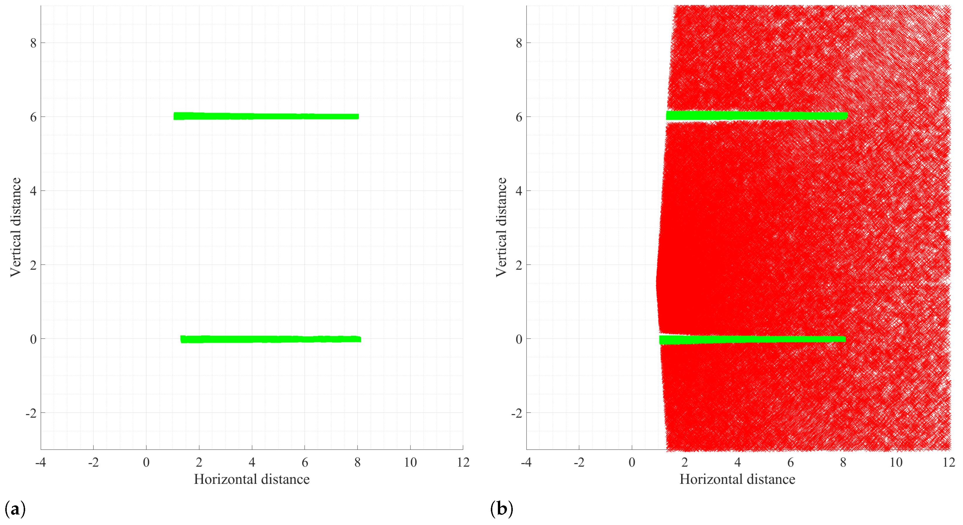
The scenarios consisted of four steps to identify the occurrence and elimination of mutual interference, and for each step, two LIDAR sensors operated in a predetermined mode. The training phase was carried out in each scenario first, and the mutual interference testing phases were performed later. LIDAR sensors ran and recorded measured data continuously. The analysis of recorded data shows the occurrence and influence of mutual interference.

The first step was the training phase, and normal LIDAR sensor operation was demarcated in the simulation scenarios. To specify the normal range of the distance measured by the two LIDAR sensors, this step consisted of two independent substeps. In the first substep, LIDAR sensor ⓐ was the normal operating state of the single-pulse mode, but LIDAR sensor ⓑ was an aborted state. In the second substep, they worked the opposite way. In these two substeps, we recorded the measured distance data at the normal operating LIDAR sensor for four working hours. We calculated the average distance, the maximum distance, and the minimum distance at each angle. After that, we calculated the upper and lower tolerance, as shown in Equations (1)–(5). The LIDAR sensor had two errors; one was a systematic error, and the other was a random statistical error. According to the rule of thumb, adding a slight margin to the maximum and minimum values could reduce misjudgment of the normal distance as interference.

$$\begin{array}{ccc}& & \overline{d}=\frac{1}{n}\sum _{i=1}^{i=n}{d}_i\hfill \end{array}$$

(1)

$$\begin{array}{ccc}& & d_{max}=MAX[d_1,d_2,\dots ,d_n]\hfill \end{array}$$

(2)

$$\begin{array}{ccc}& & d_{min}=MIN[d_1,d_2,\dots ,d_n]\hfill \end{array}$$

(3)

$$\begin{array}{ccc}& & d_{upper}=d_{max}+(d_{max}-\overline{d})\times 0.1\hfill \end{array}$$

(4)

$$\begin{array}{ccc}& & d_{lower}=d_{min}+(d_{min}-\overline{d})\times 0.1\hfill \end{array}$$

(5)

The second step to the fourth step was a testing phase. It examined abnormal LIDAR sensor operation in the simulation scenarios. Two LIDAR sensors were in the normal operating state and ran simultaneously. We recorded the measured distance data from the both LIDAR sensor ⓐ and ⓑ for 24 h. We analyzed the recorded data and classified out-of-tolerance distance as the interfered measurement result, as shown in Equation (6). In the second step, both LIDAR sensor ⓐ and ⓑ were operated in the single-pulse mode. In the third step, LIDAR sensor ⓐ was the coded pulse stream mode, but LIDAR sensor ⓑ was in the single-pulse mode. In the fourth step, two LIDAR sensor ⓐ and ⓑ were operated in the coded pulse stream mode.

$$f\left(d\right)=\left\{\begin{array}{cc}\mathrm{normal}\mathrm{distance}\hfill & \mathrm{if}{d}_{lower}\le d\le d_{upper}\hfill \\ \mathrm{interfered}\mathrm{distance}\hfill & \mathrm{else}.\hfill \end{array}\right.$$

(6)

5. Simulation Results

5.1. First Step: Training Phase for Making Demarcated LIDAR Sensor Operation

Figure 5, Figure 6 and Figure 7 are the results of the training phase, the first step in the simulation. They show the 2-D distance grid map acquired by LIDAR sensor ⓐ and ⓑ in each scenario. As described in Section 4, two LIDAR sensors were operated in the single-pulse mode separately. Green color-filled square symbols indicate correct distance data. Scatter plots are composed of many superimposed green color-filled square symbols. These plots show the position of the jersey barrier and another LIDAR sensor that the LIDAR sensor detects correctly, and they are exactly matched with the simulation scenarios. We calculated the upper and lower tolerance in each scenario, as shown in Equations (1)–(5).

5.2. Second Step: Occurrence of Mutual Interference between Single-Pulse Mode

Figure 8, Figure 9 and Figure 10 are the results of the second step in the simulation. As described in Section 4, two LIDAR sensors were operated in the single-pulse mode simultaneously. After simulation, we analyzed the recorded data and determined each measured distance to be a correct distance or out-of-tolerance incorrect distance, as shown in Equation (6). Green color-filled square symbols indicate correct distance data, and red cross symbols indicate incorrect distance data. Correct positions indicate LIDAR sensors carry out detections correctly. However, wrong positions indicate that one LIDAR sensor is affected by another LIDAR sensor, which is called a ghost target. The scanning LIDAR sensor uses a spherical coordinate system to represent an object’s distance. The closer to the LIDAR sensor, the higher the density of the azimuthal angle and the higher the distance data density.

The six figures show that both LIDAR sensors operated simultaneously in single-pulse mode, and incorrect distance due to mutual interference was measured in both LIDAR sensors ⓐ and ⓑ. As the single-pulse mode calculated the distance using all of the received reflected waves, the laser pulse transmitted by itself was reflected and received. Furthermore, the laser pulse transmitted by another LIDAR sensor, reflected, and received was used for distance calculation. Due to this, when other LIDAR sensors operated within a sufficient effective distance, mutual interference occurred, as shown in these figures.

5.3. Third Step: Occurrence of Mutual Interference in Single-Pulse Mode and Elimination in Coded Pulse Stream Mode

Figure 11, Figure 12 and Figure 13 are the results of the third step in the simulation. They show the 2-D distance grid map acquired by LIDAR sensor ⓐ and ⓑ in each scenario. As described in Section 4, two LIDAR sensors were operated simultaneously, but LIDAR sensor ⓐ was operated in the coded pulse stream mode and LIDAR sensor ⓑ was operated in the single-pulse mode. After simulation, we analyzed and determined the recorded data, as shown in Equation (6), and plotted correct distances as green color-filled square symbols and incorrect distances as red cross symbols.

In the second step, the two LIDAR sensors operated in single-pulse mode. However, in the third step, only LIDAR sensor ⓑ operated in single-pulse mode, and LIDAR sensor ⓐ operated in coded pulse stream mode. The coded pulse stream mode operated differently from the single-pulse mode in two aspects. Multiple pulses were used in the coded pulse stream mode to measure the distance to one place. Even if multiple pulses were received using the code generated by a specific rule for this pulse information, it was possible to distinguish one’s pulses. In this simulation, as the LIDAR sensor ⓐ transmitted 27 pulses to one target point, the many reflected waves were received by LIDAR sensor ⓑ. LIDAR ⓑ was able to receive 28 reflected pulses from one target point. One of them was its own reflected pulse, and 27 pulses were from LIDAR sensor ⓐ. These higher reflected pulses led to higher mutual interference, and then LIDAR sensor ⓑ had much more mutual interference than the second step. On the other hand, even when the reflected wave of the laser pulse emitted from LIDAR sensor ⓑ was received by LIDAR sensor ⓐ, it did not decode the spreading code and was removed, so there was no mutual interference in LIDAR sensor ⓐ.

5.4. Spatial and Temporal Locality of Mutual Interference

Table 9. Occurrence of consecutive mutual interference in a line on the LIDAR sensor ⓑ.

Scene	Mode	1	2	3	4	5	6	7	8	9	10	11	12	13	14	15	16	17	18	19	20
# 1	Single-pulse	3582	2097	869	725	596	424	360	352	275	219	189	173	112	68	52	51	45	33	3	0
	Coded pulses	4,918,635	90,564	15,602	11,425	5681	1762	889	808	483	322	284	240	210	189	178	156	112	74	70	45
# 2	Single-pulse	21,901	2175	1129	560	437	163	102	70	67	61	41	10	6	5	0	1	1	0	0	0
	Coded pulses	129,496	11,168	2181	755	625	615	562	289	263	225	199	134	90	79	41	1	1	0	0	0
# 3	Single-pulse	2088	1171	1107	518	473	409	369	314	293	261	207	132	102	67	59	59	33	22	0	0
	Coded pulses	357,578	43,521	13,620	5773	3056	2023	1120	922	453	395	393	256	171	170	109	74	58	16	0	0

and Figure 14a show the occurrence of interference in consecutive interfered angles from the result of LIDAR sensor ⓑ in the second and third steps. Mutual interferences mostly occurred in a single angle on the same scan line. In some cases, mutual interferences occurred in up to 20 consecutive angles. The results show that interference had temporal locality. If a particular angle interfered at a given time, then it was likely that nearby angles would interfere soon. Single mutual interference can be ignored as noise or error. It is hard to ignore consecutive mutual interference on the same line because the real object is possible.

Table 10. Occurrence of consecutive mutual interference at the same angle on the LIDAR sensor ⓑ.

Scene	Mode	1	2	3	4	5	6	7	8	9	10	11	12
# 1	Single-pulse	21,669	1628	221	214	101	77	56	0	0	0	0	0
	Coded pulses	2085	1448	346	267	155	138	44	0	0	0	0	0
# 2	Single-pulse	720	211	155	147	30	29	14	0	0	0	0	0
	Coded pulses	1283	617	532	198	149	129	84	83	73	65	12	6
# 3	Single-pulse	8793	1051	455	262	201	106	53	32	30	14	0	0
	Coded pulses	9992	564	491	393	118	51	35	18	8	0	0	0

and Figure 14b show how long the event occurred in the same angles in the consecutive interfered lines from the result of sensor ⓑ in the second and third steps. Mutual interferences mostly occurred in single lines on the same scan angle. In some cases, mutual interferences occurred in up to 12 consecutive lines at the same scan angle. The results show that interference had spatial locality. If a particular line interfered at a given time, the same location would likely interfere shortly. Single mutual interference can be ignored as noise or error. It is hard to ignore consecutive mutual interference at the same angle because the real object is possible.

5.5. Fourth Step: Elimination of Mutual Interference between Coded Pulse Stream Modes

Figure 15, Figure 16 and Figure 17 are the results of the fourth step in the simulation. They show the (2-D) distance grid map acquired by LIDAR sensor ⓐ and ⓑ in each scenario. As described in Section 4, two LIDAR sensors were operated simultaneously in the coded pulse stream mode. After simulation, we analyzed and determined the recorded data, as shown in Equation (6), and plotted correct distances as green color-filled square symbols and incorrect distances as red cross symbols.

In the fourth step, two LIDAR sensors operated in the same coded pulse stream mode, and they only transmitted and received pulse streams generated by their own specific rules and ignored any others. Even if multiple reflected pulse streams were received by sending multiple pulses to one target from another LIDAR sensor, any signals that did not conform to their rules were removed. Eventually, mutual interference did not occur. In addition, since the distance to a single target was calculated using multiple measurement results instead of one, the distance accuracy was significantly improved [40,41].

6. Conclusions

Active sensors using a wireless domain, such as a radar or a LIDAR sensor, are not free from mutual interference. In the EU, through the MOSAIM project, a study was performed on how mutual interference occurs in vehicle radar sensors. It confirmed that direct and indirect mutual interference could occur in various environments where a vehicle can drive. Unlike a radar sensor, a LIDAR sensor has a very small divergence angle, and direct mutual interferences rarely occur. Since a LIDAR sensor creates a significant intensity of reflected waves compared to a radar sensor, indirect mutual interference is likely to occur. Several preceding studies on the occurrence and resolution of mutual interference in LIDAR sensors were limited to using a single plane.

We performed simulations in which a LIDAR sensor operated in three scenarios where indirect mutual interference occurred in a radar sensor and confirmed that mutual interference could occur in all situations. These mutual interferences have temporal and spatial locality that could lead to real objects. In this study, these simulations showed that mutual interference occurs in LIDAR sensors using multi-planes and can be effectively prevented by using a coded pulse stream. The coded pulse stream method proposed in this paper randomly generates necessary information and performs encoding and decoding processes based on this. It is shown that the alien signals that caused mutual interference were very effectively removed. It is necessary to study the coded pulse stream so that it can be used when there are many LiDAR sensors in a dense space in the future. Furthermore, it is necessary to study side effects that may occur when using coded pulse streams. Due to the significant differences between the simulations and the actual environment, the signal reflected by irregular objects can destroy the encoded pulse stream in reality. So, LIDAR sensors cannot decode the received encoded pulse stream correctly.

References

1. De Ponte Müller, F. Survey on ranging sensors and cooperative techniques for relative positioning of vehicles. Sensors 2017, 17, 271. [Google Scholar] [CrossRef] [PubMed] [Green Version]
2. Shi, W.; Alawieh, M.B.; Li, X.; Yu, H. Algorithm and hardware implementation for visual perception system in autonomous vehicle: A survey. Integration 2017, 59, 148–156. [Google Scholar] [CrossRef]
3. Boulay, P.; Debray, A. LiDAR for Automotive and Indurstrial Applications 2021; Report; Yole Development: Lyon-Villeurbanne, France, 2021. [Google Scholar]
4. Van Nam, D.; Gon-Woo, K. Solid-State LiDAR based-SLAM: A Concise Review and Application. In Proceedings of the 2021 IEEE International Conference on Big Data and Smart Computing (BigComp), Bangkok, Thailand, 17–20 January 2021; IEEE: Bangkok, Thailand, 2021; pp. 302–305. [Google Scholar]
5. Li, N.; Ho, C.P.; Wang, I.T.; Pitchappa, P.; Fu, Y.H.; Zhu, Y.; Lee, L.Y.T. Spectral imaging and spectral LIDAR systems: Moving toward compact nanophotonics-based sensing. Nanophotonics 2021, 10, 1437–1467. [Google Scholar] [CrossRef]
6. Bi, S.; Yuan, C.; Liu, C.; Cheng, J.; Wang, W.; Cai, Y. A Survey of Low-Cost 3D Laser Scanning Technology. Appl. Sci. 2021, 11, 3938. [Google Scholar] [CrossRef]
7. Roriz, R.; Cabral, J.; Gomes, T. Automotive LiDAR Technology: A Survey. IEEE Trans. Intell. Transp. Syst. 2021, 1–16. [Google Scholar] [CrossRef]
8. Mitropoulos, L.K.; Prevedouros, P.D.; Yu, X.A.; Nathanail, E.G. A Fuzzy and a Monte Carlo simulation approach to assess sustainability and rank vehicles in urban environment. Transp. Res. Procedia 2017, 24, 296–303. [Google Scholar] [CrossRef]
9. Martino, L.; Read, J.; Elvira, V.; Louzada, F. Cooperative parallel particle filters for online model selection and applications to urban mobility. Digit. Signal Process. 2017, 60, 172–185. [Google Scholar] [CrossRef] [Green Version]
10. Bastos, D.; Monteiro, P.P.; Oliveira, A.S.; Drummond, M.V. An Overview of LiDAR Requirements and Techniques for Autonomous Driving. In Proceedings of the 2021 Telecoms Conference (ConfTELE), Leiria, Portugal, 11–12 February 2021; IEEE: Leiria, Portugal, 2021; pp. 1–6. [Google Scholar]
11. Brooker, G.M. Mutual Interference of Millimeter–Wave RADAR Systems. IEEE Trans. Electromagn. Compat. 2007, 49, 170–181. [Google Scholar] [CrossRef]
12. Alland, S.; Stark, W.; Ali, M.; Hegde, M. Interference in automotive radar systems: Characteristics, mitigation techniques, and current and future research. IEEE Signal Process. Mag. 2019, 36, 45–59. [Google Scholar] [CrossRef]
13. Aydogdu, C.; Keskin, M.F.; Carvajal, G.K.; Eriksson, O.; Hellsten, H.; Herbertsson, H.; Nilsson, E.; Rydstrom, M.; Vanas, K.; Wymeersch, H. Radar interference mitigation for automated driving: Exploring proactive strategies. IEEE Signal Process. Mag. 2020, 37, 72–84. [Google Scholar] [CrossRef]
14. Kui, L.; Huang, S.; Feng, Z. Interference Analysis for mmWave Automotive Radar Considering Blockage Effect. Sensors 2021, 21, 3962. [Google Scholar] [CrossRef] [PubMed]
15. Kalman, R.E. A new approach to linear filtering and prediction problems. J. Basic Eng. Mar. 1960, 82, 35–45. [Google Scholar] [CrossRef] [Green Version]
16. Carvalho, C.M.; Johannes, M.S.; Lopes, H.F.; Polson, N.G. Particle learning and smoothing. Stat. Sci. 2010, 25, 88–106. [Google Scholar] [CrossRef] [Green Version]
17. Zhao, F.; Jiang, H.; Liu, Z. Recent development of automotive LiDAR technology, industry and trends. In Proceedings of the Eleventh International Conference on Digital Image Processing (ICDIP 2019), Guangzhou, China, 10–13 May 2019; International Society for Optics and Photonics: Bellingham, WA, USA, 2019; Volume 11179, p. 111794A. [Google Scholar]
18. Fischer, C.; Ahrholdt, M.; Ossowska, A.; Kunert, M.; John, A.; Pietsch, R.; Bodereau, F.; Hildebrandt, J.; Blöcher, H.; Meinel, H. Study Report on Relevant Scenarios and Applications and Requirements Specifications; Rreport; The MOSARIM Consortium: Leonberg, Germany, 2010. [Google Scholar]
19. Ahrholdt, M.; Bodereau, F.; Fischer, C.; Goppelt, M.; Pietsch, R.; John, A.; Ossowska, A.; Kunert, M. Use Cases Description List for Simulation Scenarios; Rreport; The MOSARIM Consortium: Leonberg, Germany, 2010. [Google Scholar]
20. Schipper, T. Multi-Interference Modeling and Effects; Rreport; The MOSARIM Consortium: Leonberg, Germany, 2012. [Google Scholar]
21. Aydogdu, C.; Keskin, M.F.; Garcia, N.; Wymeersch, H.; Bliss, D.W. RadChat: Spectrum sharing for automotive radar interference mitigation. IEEE Trans. Intell. Transp. Syst. 2019, 22, 416–429. [Google Scholar] [CrossRef] [Green Version]
22. Schipper, T. Simulation of Effects and Impact of Environment, Traffic Participants and Infrastructure; Rreport; The MOSARIM Consortium: Leonberg, Germany, 2012. [Google Scholar]
23. Goppelt, M.; Blöcher, H.L.; Menzel, W. Automotive RADAR–Investigation of Mutual Interference Mechanisms. Adv. Radio Sci. 2010, 8, 55–60. [Google Scholar] [CrossRef] [Green Version]
24. Kirmani, A.; Benedetti, A.; Chou, P.A. SPUMIC: Simultaneous Phase Unwrapping and Multipath Interference Cancellation in Time–of–Flight Cameras using Spectral Methods. In Proceedings of the 2013 IEEE International Conference on Multimedia and Expo (ICME’13), San Jose, CA, USA, 15–19 July 2013; IEEE: San Jose, CA, USA, 2013; pp. 1–6. [Google Scholar]
25. Goppelt, M.; Blocher, H.L.; Menzel, W. Analytical Investigation of Mutual Interference between Automotive FMCW RADAR Sensors. In Proceedings of the 2011 IEEE Microwave Conference (GeMIC’11), Darmstadt, Germany, 14–16 March 2011; IEEE: Darmstadt, Germany, 2011; pp. 1–4. [Google Scholar]
26. McManamon, P.F. Review of LADAR: A Historic, Yet Emerging, Sensor Technology with Rich Phenomenology. Opt. Eng. 2012, 51, 060901. [Google Scholar] [CrossRef] [Green Version]
27. Dorrington, A.A.; Godbaz, J.P.; Cree, M.J.; Payne, A.D.; Streeter, L.V. Separating True Range Measurements from Multi-Path and Scattering Interference in Commercial Range Cameras. In Proceedings of SPIE—The International Society for Optical Engineering; SPIE: Bellingham, WA, USA, 2011; p. 786404. [Google Scholar]
28. Falie, D.; Buzuloiu, V. Noise Characteristics of 3D Time–of–Flight Cameras. In Proceedings of the 2007 IEEE International Symposium on Signals, Circuits and Systems (ISSCS’07), Iasi, Romania, 13–14 July 2007; IEEE: Iasi, Romania, 2007; Volume 1, pp. 1–4. [Google Scholar]
29. Guðmundsson, S.Á.; Aanæs, H.; Larsen, R. Environmental Effects on Measurement Uncertainties of Time–of–Flight Cameras. In Proceedings of the 2007 IEEE International Symposium on Signals, Circuits and Systems (ISSCS’07), Iasi, Romania, 13–14 July 2007; IEEE: Iasi, Romania, 2007; Volume 1, pp. 1–4. [Google Scholar]
30. Kim, G.; Eom, J.; Park, S.; Park, Y. Occurrence and Characteristics of Mutual Interference between LIDAR Scanners. In Proceedings of SPIE—Photon Counting Applications 2015; International Society for Optics and Photonics: San Diego, CA, USA, 2015; p. 95040K. [Google Scholar] [CrossRef]
31. Kim, G.; Eom, J.; Park, Y. Investigation on the Occurrence of Mutual Interference between Pulsed Terrestrial LIDAR Scanners. In Proceedings of the 2015 IEEE Intelligent Vehicles Symposium (IV), Seoul, Korea, 28 June 28–1 July 2015; IEEE: Seoul, Korea, 2015; pp. 437–442. [Google Scholar]
32. Kim, G.; Eom, J.; Hur, S.; Park, Y. Analysis on the Characteristics of Mutual Interference between Pulsed Terrestrial LIDAR Scanners. In Proceedings of the 2015 IEEE International Geoscience and Remote Sensing Symposium (IGARSS), Milan, Italy, 26–31 July 2015; IEEE: Milan, Italy, 2015; pp. 2151–2154. [Google Scholar]
33. Eom, J.; Kim, G.; Hur, S.; Park, Y. Assessment of Mutual Interference Potential and Impact with Off-the-Shelf Mobile LIDAR. In Advanced Photonics 2018 (BGPP, IPR, NP, NOMA, Sensors, Networks, SPPCom, SOF); Optical Society of America: Irvine, CA, USA, 2018 2018; p. JTu2A.66. [Google Scholar]
34. Martins, P.M.S.B. Interference Analysis in Time of Flight LiDARs. Master’s Thesis, Universidade de Aveiro, Aveiro, Portugal, 2019. [Google Scholar]
35. Popko, G.B.; Bao, Y.; Gaylord, T.K.; Valenta, C.R. Beam path intersections between two coplanar lidar scanners. Opt. Eng. 2019, 58, 033103. [Google Scholar] [CrossRef]
36. Popko, G.B.; Gaylord, T.K.; Valenta, C.R. Geometric approximation model of inter-lidar interference. Opt. Eng. 2020, 59, 033104. [Google Scholar] [CrossRef]
37. Hwang, I.P.; Lee, C.H. Mutual interferences of a true-random LiDAR with other LiDAR signals. IEEE Access 2020, 8, 124123–124133. [Google Scholar] [CrossRef]
38. Kawata, H.; Kamimura, S.; Ohya, A.; Iijima, J.; Yuta, S. Advanced Functions of the Scanning Laser Range Sensor for Environment Recognition in Mobile Robots. In Proceedings of the 2006 IEEE International Conference on Multisensor Fusion and Integration for Intelligent Systems, Heidelberg, Germany, 3–6 September 2006; IEEE: Heidelberg, Germany, 2006; pp. 414–419. [Google Scholar]
39. Lo, F.W.; Yang, G.C.; Lin, W.Y.; Glesk, I.; Kwong, W.C. 2-D optical-CDMA modulation with hard-limiting for automotive time-of-flight LIDAR. IEEE Photon. J. 2021, 13, 7200111. [Google Scholar] [CrossRef]
40. Kim, G.; Park, Y. Independent Biaxial Scanning Light Detection and Ranging System Based on Coded Laser Pulses without Idle Listening Time. Sensors 2018, 18, 2943. [Google Scholar] [CrossRef] [PubMed] [Green Version]
41. Kim, G.; Ashraf, I.; Eom, J.; Park, Y. Concurrent Firing Light Detection and Ranging System for Autonomous Vehicles. Remote Sens. 2021, 13, 1767. [Google Scholar] [CrossRef]
42. Ghillino, E.; Virgillito, E.; Mena, P.V.; Scarmozzino, R.; Stoffer, R.; Richards, D.; Ghiasi, A.; Ferrari, A.; Cantono, M.; Carena, A.; et al. The synopsys software environment to design and simulate photonic integrated circuits: A case study for 400 g transmission. In Proceedings of the 2018 20th International Conference on Transparent Optical Networks (ICTON), Bucharest, Romania, 1–5 July 2018; IEEE: Bucharest, Romania, 2018; pp. 1–4. [Google Scholar]
Figure 1. Normal direct time-of-flight in a LIDAR sensor. A LIDAR sensor measures distance by actively emitting an object with a laser pulse and a receiver that is sensitive to the laser’s wavelength to capture the reflected laser pulse. The sensor measures the time-of-flight Δ t between when the laser pulse is emitted and when the reflected laser pulse is received by the sensor. The time-of-flight is proportional to twice the distance between the sensor and the object (round-trip); therefore, the distance can be estimated as d i s t a n c e = c Δ t 2 , where c is the speed of light. (a) Normal direct time-of-flight situation; (b) normal direct time-of-flight measurement.
Remotesensing 14 01129 g001
Figure 2. Interfered direct time-of-flight in the LIDAR sensor. This LIDAR sensor and other LIDAR sensors emitted a laser pulse to measure the distance of an object. This LIDAR sensor received several reflected laser pulses within a specific measuring time. The first received laser pulse is a direct laser pulse emitted from another LIDAR sensor. The second received laser pulse is its own reflected laser pulse. The third received laser pulse is a reflected laser pulse emitted from another LIDAR sensor. All these received laser waveforms have similar pulse shapes with different amplitudes. Therefore, the LIDAR sensor cannot distinguish which laser pulse is its own laser pulse. (a) Interfered direct time-of-flight situation; (b) interfered direct time-of-flight measurement.
Remotesensing 14 01129 g002
Figure 3. Signal processing aspect of concurrent firing LIDAR sensor.
Remotesensing 14 01129 g003
Figure 4. Simulation scenarios. Black thick lines are jersey barriers, black dotted lines are lane lines, black arrows show moving direction of vehicle, blue and red dotted lines are boundaries of scanning area. (a) Scene #1: one vehicle with LIDAR sensor and another vehicle with LIDAR sensor are approaching each other and going along a jersey barrier; (b) scene #2: one vehicle with LIDAR sensor is following vehicle ahead with LIDAR sensor and going along a jersey barrier; and (c) scene #3: one vehicle with LIDAR sensor and another vehicle with LIDAR sensor are driving parallel along a jersey barrier.
Remotesensing 14 01129 g004
Figure 5. Distance grid maps of scene #1: two vehicles are approaching each other and going along a jersey barrier. (a) From LIDAR sensor ’s point of view at near top-right corner; (b) LIDAR sensor ’s point of view at near bottom-left corner.
Remotesensing 14 01129 g005
Figure 6. Distance grid maps of scene #2: one vehicle is following vehicle ahead and going along a jersey barrier. (a) From LIDAR sensor ’s point of view at near bottom-right corner; (b) LIDAR sensor ’s point of view at near bottom-left corner.
Remotesensing 14 01129 g006
Figure 7. Distance grid maps of the scene #3: one vehicle with LIDAR sensor and another vehicle with LIDAR sensor are driving parallel along a jersey barrier. (a) From LIDAR sensor ’s point of view at near top-left corner; (b) LIDAR sensor ’s point of view at near bottom-left corner.
Remotesensing 14 01129 g007
Figure 8. Distance grid maps of scene #1 show correct distances and incorrect distances measured by each LIDAR sensor in the second step. (a) From LIDAR sensor ’s point of view; (b) LIDAR sensor ’s point of view.
Remotesensing 14 01129 g008
Figure 9. Distance grid maps of scene #2 show correct distances and incorrect distances measured by each LIDAR sensor in the second step. (a) From LIDAR sensor ’s point of view; (b) LIDAR sensor ’s point of view.
Remotesensing 14 01129 g009
Figure 10. Distance grid maps of scene #3 show correct distances and incorrect distances measured by each LIDAR sensor in the second step.(a) From LIDAR sensor ’s point of view; (b) LIDAR sensor ’s point of view.
Remotesensing 14 01129 g010
Figure 11. Distance grid maps of scene #1 show correct distances and incorrect distances measured by each LIDAR sensor in the third step. (a) From LIDAR sensor ’s point of view; (b) LIDAR sensor ’s point of view.
Remotesensing 14 01129 g011
Figure 12. Distance grid maps of scene #2 show correct distances and incorrect distances measured by each LIDAR sensor in the third step.(a) From LIDAR sensor ’s point of view; (b) the LIDAR sensor ’s point of view.
Remotesensing 14 01129 g012
Figure 13. Distance grid maps of scene #3 show correct distances and incorrect distances measured by each LIDAR sensor in the third step. (a) From LIDAR sensor ’s point of view; (b) LIDAR sensor ’s point of view.
Remotesensing 14 01129 g013
Figure 14. Occurrence of consecutive mutual interference. (a) Consecutive mutual interference in a line; (b) consecutive mutual interference at the same angle.
Remotesensing 14 01129 g014
Figure 15. Two-dimensional distance grid maps of scene #1 show correct distances and incorrect distances measured by each LIDAR sensor in the fourth step. (a) From LIDAR sensor ’s point of view; (b) LIDAR sensor ’s point of view.
Remotesensing 14 01129 g015
Figure 16. Two-dimensional distance grid maps of scene #2 show correct distances and incorrect distances measured by each LIDAR sensor in the fourth step. (a) From LIDAR sensor ’s point of view; (b) LIDAR sensor ’s point of view.
Remotesensing 14 01129 g016
Figure 17. Two-dimensional distance grid maps of scene #3 show correct distances and incorrect distances measured by each LIDAR sensor in the fourth step. (a) From LIDAR sensor ’s point of view; (b) LIDAR sensor ’s point of view.
Remotesensing 14 01129 g017