Enhanced Chlorophyll-a in the Coastal Waters near the Eastern Guangdong during the Downwelling Favorable Wind Period

Abstract

Phytoplankton dynamics, which are highly sensitive to the ecosystem condition and change, are different in coastal waters and open ocean. Previous researches mainly focused on the open ocean dynamic in the South China Sea (SCS), but few research on the Eastern Guangdong (EGD), especially during a period of downwelling-favorable winds. In fact, the influence of topographic irregularities, downwelling, continental outflows, and cold, nutrient-rich currents from Fujian-Zhejiang coastal waters (ZFC) of the East China Sea (ECS) on the spatial distribution of Chlorophyll a (Chl a) in EGD coastal waters could be significant. This study utilized ocean color time series and meteorological and hydrographic data jointly from July 2002 to June 2020 to investigate the heterogeneous regional specific distribution pattern of Chl a in EGD and the environmental determinants in different regions subdivided by water depth. Then the temporal and spatial distribution pattern of Chl a in EGD in winter were discussed in detail by applying an Empirical Orthogonal Function (EOF) analysis, GaoFeng-1 (GF-1) satellite data and in situ measured dataset. The sea surface temperature (SST) in February was negatively related with Chl a in shallow coastal waters less than 60 m deep due to the nutrient-rich, cold waters from ZFC. The monthly mean photosynthetically active radiation (PAR) and precipitation showed significant effects on the phytoplankton growth over regions with a depth less than 10 m. An area with higher Chl a concentration in the downwelling zone were detected in winter. By an examining the temporal variability in meridional distribution of the mean Chl a at 22.41°N and 22.21°N, a symmetrical peak was observed. The coastal fronts extended southwestward from the southeastern coast of Guangdong Province to Dangan Island in the SCS. In addition, a cross-shelf filament was detected near the coast of Shanwei, Guangdong, China on 8 January 2020.

1. Introduction

The South China Sea (SCS) circulation are mainly driven by the East Asian Monsoon [1]. The oceanographic studies on the SCS have been centered on the open ocean dynamic, the summer upwelling phenomena or the interaction between the Pearl River plume and the coastal current for a few decades [2,3,4]. Liu [5] developed a three-dimensional numerical model with coupled physics and biogeochemistry to illustrate the relationship between the nutrient upwelling and phytoplankton growth in the SCS. Chen [6] discussed the effects of upwelling on the phytoplankton blooms in the SCS. Zhang [7] examined the variability of chlorophyll a (Chl a) in the open SCS by using observations from two Bio-Argo floats. He [8] analyzed the influence of the intense mesoscale eddies on Chl a in summer in the western South China Sea (WSCS) in summer by using historical in situ observations, satellite-derived Chl a and eddy data. Kuo [9] analyzed the spatial and temporal variation of Chl in SCS by using the Empirical Orthogonal Function (EOF) analysis. However, the results mainly focused on Chl a plume along the Vietnam coast in summer and the warm Kuroshio water intrusion to the Luzon Strait. Such a conclusion based on the relationship between the EOF results of Chl a and sea surface temperature (SST) in this literature could only be applied to open ocean. For the EGD coastal waters, the nutrient-rich, cold waters from Fujian-Zhejiang coastal waters (ZFC) of the East China Sea (ECS) could affect SST and Chl a significantly which may make the story here is different. Maisyarah [10] analyzed the relationship between ENSO and Chlorophyll-a, and the study area was the southern area of the SCS. Many researches have been carried out in the open ocean of the SCS. However, little research on the temporal and spatial dynamics of phytoplankton along the Eastern Guangdong (EGD) coast during periods of strong downwelling favorable wind. It is well known that Chl a dynamics in the coastal waters are very important not only to an effective coastal zone management, but also to algal bloom, fishery activities, the pollutant dispersion, and the seafloor sediment. The extent and availability of phytoplankton biomass drives marine ecosystem trophic-structure. Phytoplankton variability is a primary driver of chemical and biological dynamics in the coastal zone, which directly affect water quality, biogeochemical cycling of reactive elements, and food supply to consumer organisms. Apparently, it is a sensitive indicator of long-term climate variability in the open ocean, but how does it vary and respond to the environmental factors in EGD coastal waters has not been understood very well. The natural changes to the local environment of each coastal water body could cause a wide range of seasonal patterns with large variability across and within coastal water bodies. Coastal zones are highly dynamic systems in the interface of ocean-climate and continental processes. Winds control the wave activities which then generate currents nearshore, while the approach directions and speeds of wind and waves show seasonal variation. The surface features of phytoplankton affected by the wind and ocean currents which in turn strongly influence the biological processes and ocean ecosystem. Meanwhile, human landscape transformations, fishing, aquaculture, river damming and diversions, introduced species, and contaminants could also change the biological process significantly. Coastal hazards can result in not only property damage but also loss of life and environmental degradation.

A systematic information base on the phytoplankton dynamics and the pattern of locally maximum Chl a near the coast of the EGD is meaningful. However, the understanding of Chl a dynamics in EGD coastal waters is still unclear and thus needs to be investigated further. It is important to figure out how Chl a dynamics responds to the prevailing winds and coastal currents in EGD coastal waters. With the development of the remote sensing techniques, the long-term satellite data has the potential to explore critical ecological variability. Satellite data is an effective data source for studying the temporal and spatial pattern of the phytoplankton dynamics in EGD coastal waters.

The purpose of the study is to analyze the temporal and spatial distribution of Chl a in coastal waters and Chl a dynamics by applying the ocean color data, meteorological and hydrographic data jointly. To identify the major important factors influencing the coastal phytoplankton variation and improve our understanding of the linkages between phytoplankton dynamics and physical environment along the EGD coast, we established a long-term Chl a time series and examining the environmental factors contribute to the variability in Chl a.

2. Materials and Method

2.1. Satellite Data Acquisition and Processing

Moderate-resolution Imaging Spectroradiometer (MODIS) Aqua and Terra between July 2002 and June 2020 were acquired from the NASA’s Level-1 and Atmosphere Archive & Distribution System (LAADS) Distributed Active Archive Center (DAAC) were applied in this study. An iterative f/Q BRDF correction [11,12] and the MUMM-based atmospheric correction [13] were utilized in the SeaWiFS data analysis system (SeaDAS, version 7.5.1, available at https://seadas.gsfc.nasa.gov/, accessed on 11 February 2022). The bands of the MODIS-Aqua sensor centered at 412, 443, 490, 510, 555 and 670 nm with 10 nm bandwidth were applied to retrieve the chlorophyll a concentration.

The L1 level of GF-1/Wide Field of View (WFV) imagery on 8 January 2020 had been applied. There are four band multi-spectral CCD cameras with a spatial resolution of about 16 m (WFV 1–4) on the board of the GF-1 satellite. These acquired images cover the spectral ranges of 450–520 nm, 520–590 nm, 630–690 nm and 770–890 nm. The spectral response functions (SRFs) can be downloaded from http://www.cresda.com, accessed on 11 February 2022.

The latest climate reanalysis ERA5 were utilized which are released by European Centre for Medium-Range Weather Forecasts (ECMWF) and carried out by using ECMWFS’ Earth System model IFS, cycle 41r2. The hourly wind speed at the height of 10 m above the sea surface with 0.25° × 0.25° resolution has 37 pressure levels, which were obtained from the Climate Data Store (https://climate.copernicus.eu/climate-reanalysis, accessed on 11 February 2022). In order to analyze the relationship between wind speed and Chl a, ERA5 data was extracted for the pixel of MODIS in EGD for the period of July 2002 and June 2020.

The monthly accumulated precipitation product applied here were generated from the 3-hourly 0.25° × 0.25° TRMM Multi-Satellite Precipitation Analysis TMPA (3B42) which was given in mm.month⁻¹. The precipitation data were obtained from http://apdrc.soest.hawaii.edu/datadoc/trmm_3b42_daily.php (accessed on 11 February 2022). In order to analyzed the relationship between precipitation and Chl a, monthly accumulated precipitation product was extracted for the pixel of MODIS in EGD for the period of December 2002 and November 2019.

The global Hybrid Coordinate ocean Model and the Navy Coupled Ocean Data Assimilation (HYCOM + NCODA) Global (1/12)° Analysis were provided by the Global Ocean Forecasting System (GOFS). The data assimilation scheme used is a three dimensional variational scheme (3DVAR) [14]. 3-hourly velocity fields for the period of July 2002 and June 2020 were extracted for the pixel of MODIS in this study.

ETOPO1 (NCEI, https://www.ngdc.noaa.gov/mgg/global/global.html, accessed on 11 February 2022) bathymetry grids at 1-arcminute resolution from the National Centers for Environmental Information were obtained. The bathymetry grids were extracted for the pixel of MODIS.

2.2. In Situ Data

The first in situ dataset comprises samples and radiative measurements collected from the Pearl River estuary on 25 January 2003, 26 January 2003, 5 January 2004, 6 January 2004, 18 May 2004, 15 August 2009, 22 October 2009, 22 November 2009, 13 December 2009, 1 February 2010, 4 July 2010, 5 June 2012, 10 December 2012, and 7 November 2013. This dataset consists of 199 apparent optical property (AOP) measurements with matching IOPs. All measurement protocols followed those recommended for SeaWiFS calibration activities (More details can be found in [15]). The water-leaving radiance was measured from the desk of a ship using a spectrometer (USB4000, Ocean Optics, Inc., Dunedin, FL, USA) following the National Aeronautics and Space Administration (NASA) ocean optics standard protocol [16,17]. The spectrometer which has been fully characterized and calibrated was used to measure radiance emanating from the sea surface at zenith angle θ (chosen as 45°). The azimuth angle φ was chosen between 90° and 180° away the sun’s azimuth. The solid-angle field of view (FOV) is 10°. The radiance reflected from a horizontal plaque having a known bi-directional reflectance (assumed to be near-Lambertian) for the solar was also recorded to estimate the incident spectral irradiance measured above the sea surface.

The second in situ dataset is from HKUST which is part of SeaBass. Four cruises, namely, HK_010301, HK_010315, HK_010426, and HK_010510, covered Port Shelter, Lamma Channel and the Pearl River estuary in February, March, April, and May 2001. For more details, see https://seabass.gsfc.nasa.gov/ (accessed on 11 February 2022). A YSI multi-parameter sonde (temperature, pH, Chl-a, turbidity) with GPS capabilities was employed to collected data. A free fall underwater profiling unit (PRR 800) was used to collect spectra data.

The water samples for measuring Chl a were collected from the surface layer (a depth of between 30 cm and 50 cm) and filtered through 25-mm Whatman GF/F filters under a low vacuum. The filters were measured using a 90% acetone method in a pre-calibrated Turner Design 10 fluorometer [18].

A real time water quality buoy (GD3810; 3 m diameter) operated by Chaozhou Natural Resources Bureau, Guangdong, China, is maintained in Qingyu, Chaozhou, Guangdong, China (23°32.20′ N,117°3.70′ E, see Figure 1). At this location, the water depth is about 10 m. A buoy (FZS5-1) equipped with a YSI EXO2 water quality sonde which fitted with a fluorometric probe was deployed between 16 April 2019 and 31 July and Chl a was measured using a fluorometer.

In addition, a real time hydrographic buoy (GD3806 denoted as S2 here; 6 m diameter) operated by Department of Natural Resources of Guangdong Province, Guangdong, China, was maintained in Honghai Bay, ShanWei, Guangdong, China (22°17.65′N,115°14.7′E, see Figure 1). A buoy (FZS6-1) equipped with a ZPulse Doppler Current Sensor (DCS 4420, Aanderaa Instruments) was utilized for the period of between 6–8 January 2020 and 20–22 February 2020.

2.3. Method

2.3.1. Model for Chl a Retrieval

The semi-analytical model of Maritorena [19] was applied to derive Chl a from Modis Satellite data. The Garver-Siegel-Maritorena used the quadratic function of Gordon [20] to invert all the IOPs simultaneously from spectral R_rs (412, 443, 490, 510, 555 and 670 nm), using a non-linear minimum square regression fit.

$$R_{rs}\left(\lambda \right)=g_1\frac{b_b\left(\lambda \right)}{a\left(\lambda \right)+b_b\left(\lambda \right)}+g_2{\left(\frac{b_b\left(\lambda \right)}{a\left(\lambda \right)+b_b\left(\lambda \right)}\right)}^2$$

(1)

where, g₁, g₂ are the value of 0.0949 and 0.0794 respectively, a (m⁻¹) is the total absorption, which is the sum of the individual contribution of pure sea-water, phytoplankton a_ɸ (m⁻¹), and colored detrital matter a_y (m⁻¹); b_b (m⁻¹) represents the sum of the backscattering coefficients of pure seawater b_sw (m⁻¹) and particulate b_bp (m⁻¹). The parameters in the model including the Chl a specific absorption coefficient of phytoplankton, the spectral slope for a_y and b_bp were set as previously described Maritorena [19].

Because only four bands can be applied to retrieve Chl a information for GF-1 (450–520 nm, 520–590 nm, 630–690 nm and 770–890 nm). An empirical model was developed to derive Chl a from GF-1 data by using in situ dataset collected in study area.

$$Ch{l}_{model}=d/\left(a+b\cdot sin\left(m\cdot pi\cdot x\cdot y\right)\right)+c\cdot exp(-{\left(w·y\right)}^2)$$

(2)

where x is the ratio of the reflectance of the 1st band and the 2nd band; y is the ratio of the reflectance of the 1st band and the 3th band; a, b, c, m, and w are the empirical constants calculated based on the in situ data, and a was set to 32.93, b was set as 1.405; c was set as −32.4; m was set to 0.4373; w was set to 0.1109; d was set as 34.335.

2.3.2. Model for K_d (490) Retrieval

For K_d (490) estimation, Wang’s model [21] was applied in this study

$$\begin{array}{l}{K}_d\left(490\right)=\left(1-W\right){K_d}^{clear}\left(490\right)+W{K_d}^{turbid}\left(490\right)\\ \begin{array}{cc}with& W=-1.175+4.512R_{rs}\left(670\right)/R_{rs}\left(490\right)\end{array}\end{array}$$

(3)

where R_rs is remote sensing reflectance with a unit of sr⁻¹. K_d^clear (490) denotes the model for open clear water, and K_d^turbid (490) denotes the model for coastal turbid water).

2.3.3. Ekman Pumping

The Ekman pumping velocity was computed directly from the following equation [22,23]:

$$w=\frac{1}{\rho f}k\mathsf{\nabla }\times \overrightarrow{\tau }$$

(4)

where ρ is the mean density of seawater, and f is the Coriolis parameter, $k$ is a unit vector, $\overrightarrow{\tau }$ is the hourly wind stress vector.

2.3.4. EOF

In order to regionalize the higher Chl a zone, Empirical orthogonal function (EOF) analysis of Chl a was applied here based on the satellite retrieved Chl a in winter during 2003–2020. The Chl a time series without land values was demeaned by subtracting the 18-year temporal mean and dividing by standard deviation of each pixel. Singular value decomposition of the Chl a was utilized to retrieve the EOF spatial components, associated eigenvalues and time-varying amplitudes. It is decomposed following the method proposed by Polovina and Howell [24]:

$$F\left(x,t\right)={{\displaystyle \sum }}^{ }{a}_i\left(t\right)c_i\left(x\right)$$

(5)

where a_i(t) is the ith principal component time-series (temporal expansion coefficients) of the coefficients of the spatial components c_i(x).

2.3.5. The Modelling Sensor Spectral Reflectance

In order to develop an empirical model of Chl a for GF-1, the spectral response function (SRFs) of GF-1 was used to simulated each band [25].

$$R_{rs}\left({\lambda }_i\right)=\frac{{\int }^{ }{\rho }_i\left(\lambda \right)R_{rs}\left(\lambda \right)d\lambda }{{\int }^{ }{\rho }_i\left(\lambda \right)d\lambda }$$

(6)

where R_rs(λ) is the remote sensing reflectance of the ith band in GF-1; ρ_i is the spectral response functions (SRFs) of the ith band; R_rs is in situ measured reflectance (sr⁻¹).

2.3.6. The Standard Deviation

In order to analyze the average long-term data on the concentration of chlorophyll a in certain seasons by region. The standard deviation (SD) is applied to see how reliable the differences between seasons are in terms of average values.

$$\mathrm{SD} = \sqrt{\frac{{\sum }_{i=1}^n(x_i-\tilde{x})}{n-1}}$$

(7)

where x_i is the value of the ith point in the data set, $\tilde{x}$ is the mean value of the data set, and n is the number of data points in the data set.

3. Results

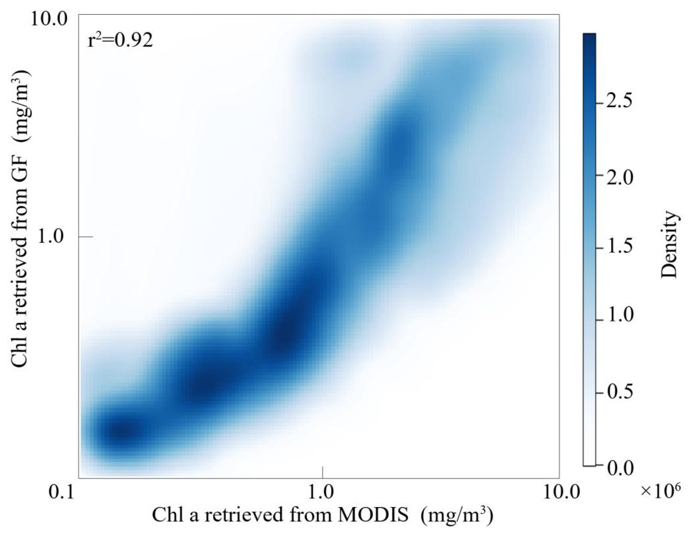
3.1. Chl a Retrieval Model Assessment

In this study, GSM was applied to estimate Chl a from MODIS satellite data. GSM was initially developed by Garver&Siegel [26], and later updated for a global application by Maritorena [19]. The model widely applied and validated [27,28,29]. In order to make sure the model also can be applied to our research area, we evaluate it by using in situ data collected in SCS (Figure 1). Figure 2a show the goodness of fit (R² = 0.73). The results are acceptable to obtain a long term Chl a from MODIS satellite dataset. However, the algorithm can not be applied to GF-1, because only four bands of Blue (0.45–0.52 μm), Green (0.52–0.59 μm), Red (0.63–0.69 μm) and Near Infrared (0.77–0.89 μm) are available from GF-1. In order to apply GSM, six bands (412, 443, 490, 510, 555 and 670 nm) are necessary. An empirical approach (Equation (2)) was used for estimating the concentrations of Chl a in order to apply GF-1 with a high spatial resolution to analyze the relatively higher Chl a zone. The retrieval algorithm was established through regression processes while using nonlinear power-law regression approaches. The goodness of fit was judged by the value of the coefficient of determination (R²) based on the in situ measured data. The comparison of the in situ vs estimated Chl a (Equation (2)) is shown in Figure 2b. R² is 0.74. It can be seen that the the scatter points are well distributed around the 1:1 line. Figure 3 shows the relationship between the retrieved Chl a from GF-1 (calculated by Equation (2)) and MODIS (calculated by Equation (1)) for 8 January 2020. The results show the r² was 0.92 (Figure 3) which indicates the empirical algorithm is effective to retrieve Chl a from GF-1. The spatial distribution pattern of Chl a in GF-1 and MODIS were significantly similar (Figure 4). In addition, GF-1 could provide more detail information.

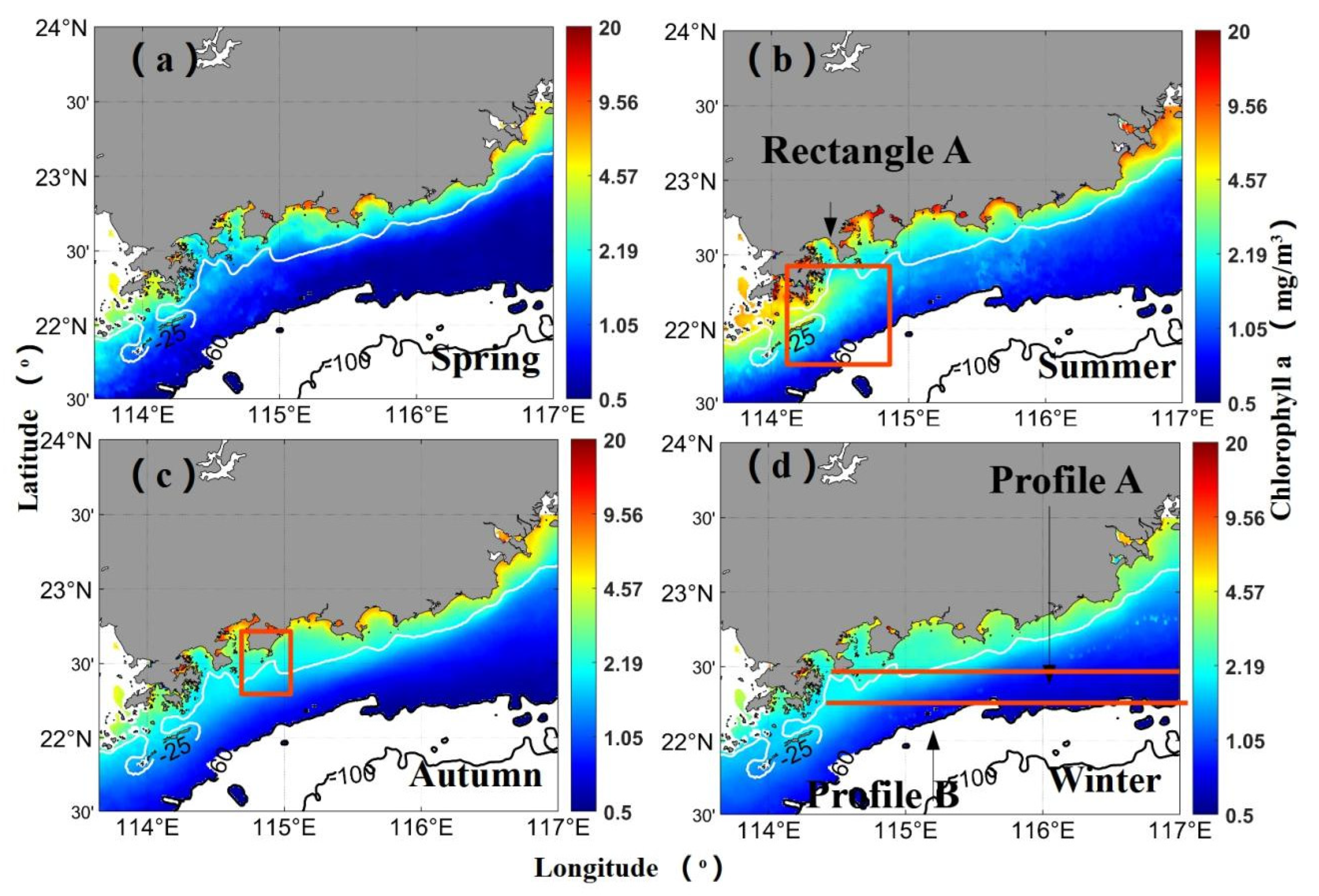
3.2. Chlorophyll a Distribution in the Coastal Waters of EGD

Figure 5 is the mean Chl a concentration in the EGD coastal water for four seasons from July 2002 and June 2020 retrieved from MODIS data. Due to the estuarine and coastal eutrophication, the Chl a is significantly high nearshore than offshore in whole year, and it rapidly decreases offshore. Nutrients are plentiful in coastal waters along China’s Guangdong Province [30,31,32]. One of the well-known effects of anthropogenic nutrient enrichment is the increase of phytoplankton biomass. Nutrient over-enrichment of coastal ecosystems is an important factor to an increase in phytoplankton biomass nearshore [33,34,35]. Chl a were obviously higher in areas of shallow water depth (<25 m) than in areas where the seafloor was deeper. Phytoplankton community generally originated from the coastal waters [36]. In order to analyze the spatial distribution of Chl a, the study area (114.3–117°E; 21.6–24°N) was subdivided into four analysis regions (with a depth shallower than 10 m denoted as region I, between 10 m to 25 m denoted as region II, 25 m to 60 m denoted as region III, and deeper than 60 m denoted as region IV). The results (

Table 1. The mean value of the Chl a (mg/m³) in four seasons from July 2002 to June 2020 (114.3–117°E; 21.6–24°N).

Region	Chl a (mg/m3)	Mean	sd	Max	Median
Region I	spring	3.55	1.27	8.10	2.33
Region I	summer	4.68	1.67	8.64	3.85
Region I	autumn	3.94	1.03	5.74	3.45
Region I	winter	3.19	0.62	4.41	2.57
Region II	spring	1.11	0.29	2.06	0.99
Region II	summer	1.38	0.36	2.67	1.39
Region II	autumn	1.43	0.27	2.03	1.44
Region II	winter	1.52	0.34	2.76	1.53
Region III	spring	0.74	0.20	1.03	0.73
Region III	summer	1.14	0.30	2.17	1.12
Region III	autumn	1.02	0.23	1.37	0.99
Region III	winter	1.13	0.19	1.44	1.10
Region IV	spring	0.19	0.12	0.52	0.25
Region IV	summer	0.34	0.10	0.58	0.30
Region IV	autumn	0.24	0.09	0.53	0.28
Region IV	winter	0.42	0.09	0.84	0.50

) show that the mean Chl a concentration in this area with a depth shallower than 10 m (region I) was significantly higher in summer (4.68 mg/m³) relative to winter (3.19 mg/m³). The seasonal change of Chl a in coastal zone exhibited in satellite data is similar with the temporal trends captured by the buoy data (located near Qingyu island, Guangdong, see Figure 6). Coastal waters conditions are generally affected by a variety of stressors, including storm water, agricultural runoff, and sewage discharge or overflows [30]. Excess nutrients loading to coastal environments can enhance phytoplankton growth and biomass [37]. It could be found that precipitation is relatively higher in summer based on the seasonal analysis of satellite retrieved precipitation from December 2002 to November 2019 (Figure 7). It in turn affected the nutrient changes. The amount of nutrients from terrestrial sources could be significantly increased by nutrient runoff from agricultural and other human activities. The heavy rainfall increased the transport of river-bond inorganic nutrients from the terrestrial system to the coast and may therefore cause phytoplankton blooms and eutrophication in the recipient coastal ecosystems. In addition, upwelling event has been observed in summer along the EGD coast. A lower temperature area near Shantou in Guangdong province can be seen in Figure 8b (Rectangle B). The coastal upwellling happened in shallow nearshore waters less than 20 m depth in summer. The nutrient in deep water could be transported to euphotic layer by upwelling currents. Another reason for the temporal pattern could be the variation of the underwater light climate. Environmental Light condition is also an important factor influencing the seasonal development of phytoplankton biomass. We compared the mean PAR (Einstein·m²/day) in four seasons based on the satellited retrieved data from July 2002 and June 2020 which showed that PAR was highest in summer (Figure 9). In addition, it can be found that SD is relatively larger in region I, especially for summer (1.67 mg/m³). Horizontal mixing in coastal water is relatively weaker due to a complex coastline and shelf topography (Gan et al. 2013; Rao and Schwab 2007). Consequently, phytoplankton biomass is prone to be patchy in the shallow waters [38]. Harmful algal bloom (HAB) was found in Daya Bay in Guangdong, Raoping in Guangdong, Dapeng Bay in Guangdong, Tolo Harbour in Hong Kong [30]. Those phytoplankton patches cause the high SD in region I. For region II in the coastal waters in Guangdong (10 m to 25 m), the SD decreased dramatically. The horizontal mixing here is stronger than in region I. In addition, the maximum of the mean value was found in winter. The strong cold coastal currents can be detected by satellite retrieved SST in winter (Figure 8). The influence of the high nutrient and cold waters from ZFC of the ECS is very significant [15,39]. SST gradually decreased from south to north along the coast of Guangdong up to Fujian. The influence of the cold currents gradually weakened from north to south [40]. Based on the SST, the thermal front of the cold water mass became week dramatically in Daya Bay. In addition, The East Asian winter monsoon is very strong in winter [41]. The physical forcing could reduce the stability of water column and enhance vertical mixing which could provide more nutrients to the euphotic zone and enable phytoplankton to grow. High Chl a was limited to coastal waters by the northeast wind along the bathymetric contour of 25 m. For the waters with a depth from 25 m to 60 m (region III), the Chl a was higher in winter and summer. The contribution of the Pearl River to the Chl a distribution in the EGD coastal waters can be found in summer (see Rectangle A in Figure 5). The pearl river plume extended from the mouth of the Pearl River estuary to the middle shelf. The high Chl a tongue affected the waters with 25 to 60 m depth significantly. Similar to the nearshore waters, the cold currents and downwelling favorable monsoon could be the main reasons to the high Chl a in winter. The strong northeast monsoon wind blowing parallel to the coast created Ekman transport that pushed surface water to the coast. The onshore flow in the surface Ekman layer created a compensating seaward submerged subsurface front. An overturning cross-shelf circulation induced by downwelling jet together with wave breaking and other nonlinear wave effects that trigger enhanced vertical mixings. The dynamic process is also related to the coastal fronts extended southwestward from the southeastern coast of Guangdong Province to Dangan Island in winter (see Figure 5d). The meridional distribution of the mean Chl a at 22.41°N and 22.21°N were given in the upper line and in the bottom line of Figure 10. Both of the curves exhibited a peak between 114.5–115°E which clear proved the significant discontinuity existed here. The width of the Chl a front tended to decrease with the latitude decreasing. The outer edge of the Chl a front is smooth and sharp. The demarcation line parallel to a coastline between lower and higher Chl a is very clear and obvious in winter. The Chl a front is intensity gradients. The northeast monsoon wind prevents the dispersion of Chlorophyll-a into the ocean. For deeper waters (>60 m; region IV), the maximum of Chl a was shown in winter. It is relatively easier for deeper water to rise to the surface when surface waters get colder which in turn bring the nutrients to sunlit areas where phytoplankton can use them.

Please note that the color scale for different seasons is different.

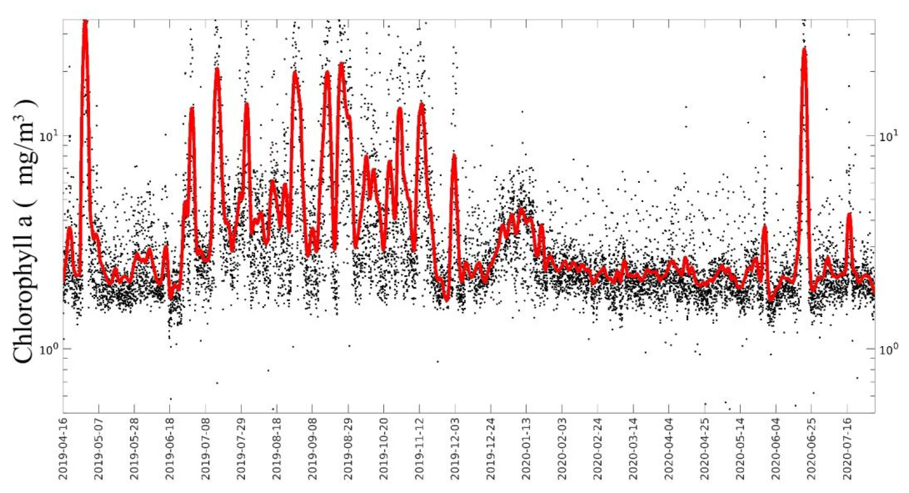
3.3. The Temporal Variation of the Mean Chl a

It was found that Chl a is highly related to Ekman Pumping in February, so time series of the mean Chl a in the coastal waters (<60 m) in the region (114.3–117°E; 21.6–24°N) in February during July 2002 and June 2020 was compared with SST, the mean Ekman Pumping velocity retrieved by ERA5 datasets, and the mean surface currents velocity simulated by HYCOM (given in Figure 11). Chl a showed an opposite trend with the mean SST and the mean Ekman pumping velocities, and an identical trend with the mean surface current velocity. The correlation between the Chl a in shallow coastal waters less than 60 m deep along the EGD coast and the mean SST, the monthly mean Ekman pumping velocities and the mean surface currents velocities were −0.79, −0.71, and 0.56 respectively. It illustrated that Chl a tended to be increased with the impact of cold water mass from ECS increasing. The nutrients in ZFC waters could be advected to the EGD coast by the strong coastal current. The lower the SST along EGD coast means more cold water was transported from ZFC to EGD. The identical trend between Chl a and currents velocities could also be considered as another evidence to prove this point. The higher velocity the more cold and nutrient-rich water were transport from ZFC to EGD. Besides, the arrival of the cold water front from ZFC can produce small bottom shear stresses there which could affect the variations of nutrient transport. In the perspective of Ekman Pumping, it could enhance the increase of Chl a for the areas less than 60 m deep. The water is mixed well top to bottom due to downwelling events. In addition, thermocline and halocline had been found at a depth of 15 m in EGD [42]. The strong Asian winter monsoon wind (blowing parallel to the coast) induced Ekman transport. The surface water was pushed to the coast. The onshore flow in the surface Ekman layer created a compensating seaward submerged subsurface front. An overturning cross-shelf circulation induced by downwelling jet together with the effects of wave breaking, other nonlinear wave effects and tides that trigger enhanced vertical mixings [43]. The effects of turbulent motion on bed shear stress can cause transport of the nutrients in shelf seas. Moreover, shelf topography in the longshore direction could be considered as an important factor to the cross-shore bottom transport. The instabilities leaded to the development of vigorous turbulent. The secondary circulation transports the coastal nutrient in subsurface and bottom waters to the open ocean.

No apparent relationship was observed between the mean Chl a in areas with depth < 60 m and the mean PAR (<60 m). However, the mean Chl a in the nearshore areas < 10 m deep was highly related to the mean PAR in the same areas (Figure 12). The correlation coefficient between the mean Chl a and the mean PAR is 0.54. For the very shallow water zone (<10 m), the nutrient is plentiful and the water column is mixed very well in those area. For the deeper coastal waters, nutrient limitation might be more frequent. It should be noted that Chl a rapidly decrease offshore (Figure 5) as well as the diffuse attenuation at 490 nm also decrease rapidly (Figure 13). Better light condition can be expected in the areas with depth > 10 m. The variation of the Chl a was mainly determined by the variation of the nutrients. The light condition is less important to the phytoplankton growth at those locations.

3.4. EOF Modes of Chl a

Based on the long term remote sensing analysis, a relatively higher Chl a zone can be detected from the southeastern coast of Guangdong Province to Dangan Island in winter. Figure 14a,c,e showed the spatial components of the first three dominant EOF modes, which totally overall accounted for 69% Chl a variability. The first mode exhibited two separated regions: the shallow nearshore waters inside the 10 m isobath and outside the 10 m isobath. For the region with the depth larger than 10 m, the spatial coefficients is relatively stable (0~0.2), indicating its higher Chl a temporal stability in respect to the shallow nearshore waters less than 10 m. The opposite trend between the shallow nearshore waters (less than 10 m) and the deeper waters is consistent with the results in Table 1. The associated temporal coefficients (Figure 14b) were relatively larger in 2005 and 2017, and least in 2007. The spatial coefficients in the shallow nearshore waters is negative. The higher the associated temporal coefficients, the lower the Chl a in those blue (negative value) spots. The mode captured the local high Chl a events in the nearshore areas of EGD in winter. The high Chl a events may due to the algal bloom. Several significant harmful algal bloom (HAB) events were found in the winter 2007 (The algal bloom events were investigated and documented by State Oceanic Administration People’s Republic of China). A bloom covered an area of 35 km² in Pinqing Lake, Shanwei, Guangdong, China from December 2 to 15, 2006. Phaeocystis was the dominant species (algal density reached 3.3 × 10⁷ cells/L). Another coastal Phaeocystis bloom event was found in Yantian Bay, Shenzhen, Guangdong, China from January 26 to 31, 2007. It covered an area of 5 km². The coastal Phaeocystis bloom had also been found in Nanao Island, Shantou on 6 February 2007 and the events lasted 30 days. The area of the blooms reached 200 km². On the contrary, no significant HAB event had been documented in this study area (EGD) during January to March 2005 and 2017. The second EOF mode (EOF2) explained 14.7% of Chl a variability. The spatial component differentiated two regions. There was a region with a higher spatial coefficients (positive values) from the southeastern coast of Guangdong Province to Dangan Island in EOF2 mode. Figure 14 shows that the region with the positive spatial coefficients was in the downwelling zone. The Ekman pumping velocity is relatively larger in winter of 2011 and 2017 (Figure 15j,p). Correspondingly, the EOF2 temporal coefficients were relatively higher during the same period. The surface water near shore was pushed against the shore, piled up and sunk in consequence of an undercurrent occurred. In addition, an alongshore current moves parallel to shore. The alongshore current that approach the shoreline at an angle near the Daya Bay and the coast of Shanwei could be turned by the convex coastline, which in turn generated a secondary circulation. It will be discussed by using a high spatial resolution satellite imagery later. The third EOF mode (EOF3) explained 8.9% of Chl a variability. The spatial coefficient was positive along the eastern coast of EGD. The nutrient and sediment waters from Fujian-Zhejiang coastal waters (ZFC) in the southern part of the East China Sea (ECS) could flow into the SCS by the strong coastal current. However, the influence of the ECS coastal water was weakened from north to south. The mode indicated the nutrient situation of the longshore current from ZFC.

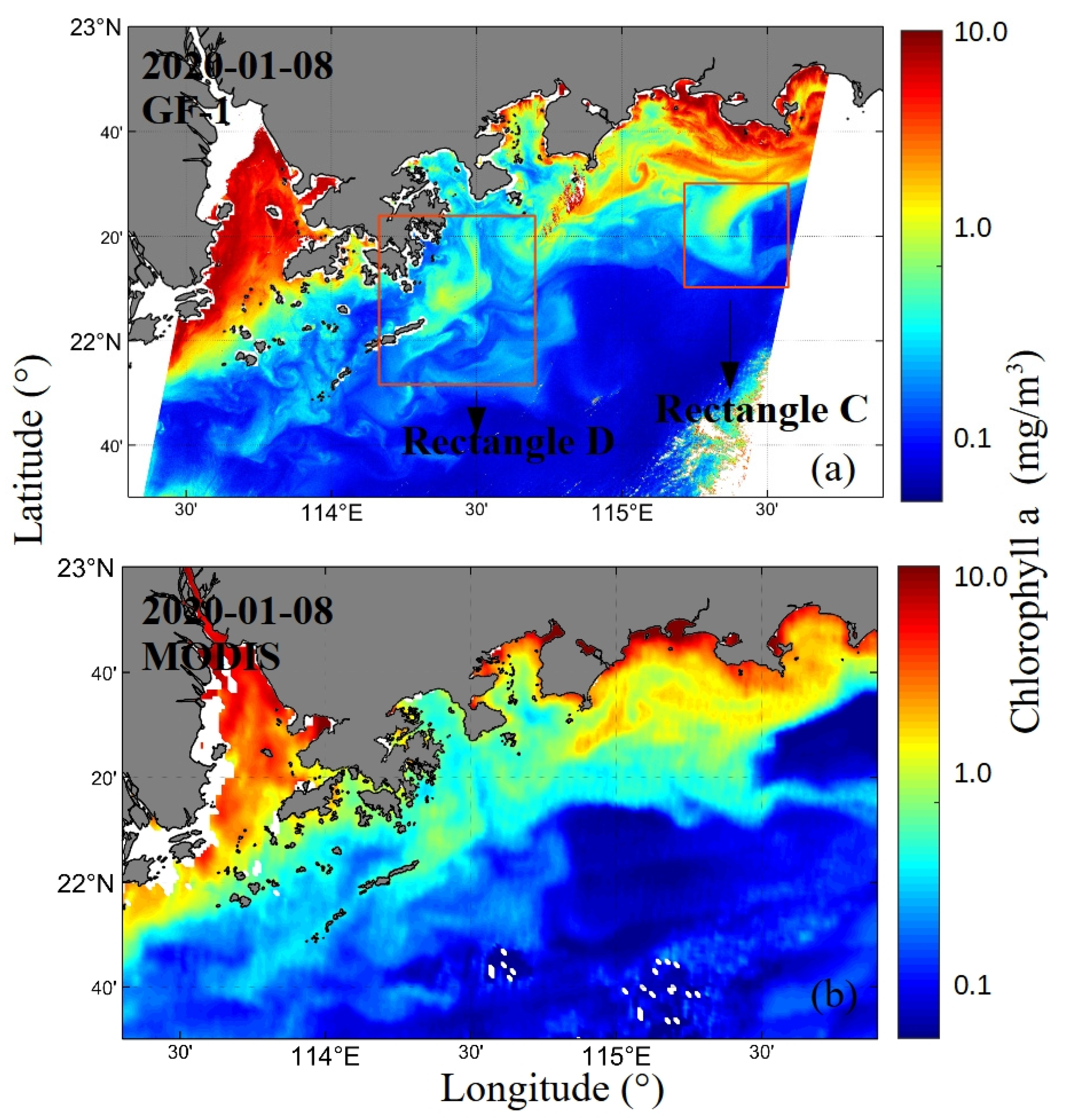
3.5. Cross-Shelf Jet Observed in GF-1

The overall purpose of this study is to figure out the temporal and spatial of Chl a in EGD during the during the downwelling favorable wind period. Based on the long term satellite observations, a relatively higher Chl a zone was detected from the southeastern coast of Guangdong Province to Dangan Island in winter. The higher Chl a zone had been found to be related to the downwelling intensity and the flows with the low temperature and high nutrients from ZFC. The coastal higher Chl a zone is a very important energetic oceanographic feature, usually occurred in the regions where the density, velocity, salinity or temperature gradient is extremely high or a significant discontinuity exist. It could play an important role in the dynamical and chemical processes. In order to improve our understanding of the distribution pattern of the high Chl a zone near Dangan Island and the coast of Shanwei in winter, a high spatial resolution satellite imagery and a daily product are applied. There two feature like pattern (Rectangle C and Rectangle D) in Chl a can be observed (Figure 5) which were also showed in EOF2 with a higher spatial coefficients (black spots) (Figure 14c). The significant cross-shelf penetrating fronts near the coast of Shanwei (Rectangle C) was also clear in SST (Rectangle E in Figure 16). The significant cross-shelf jet can be detected by the lower temperature fronts extended eastward from Honghai Bay, Guangdong to the continental shelf in deeper water. In order to analyze the effects of the coastal currents on the distribution of Chl a in Rectangle C, the surface current speed and direction at station S2 were provided in Figure 17. GF-1 images were acquired at 03:15 am (Coordinated Universal Time, UTC) 8 January 2020. Figure 17 showed the direction of the current toward the east or northeast during that time. The high Chl a near the coast of Shanwei was advected to the continental shelf with deeper water by the cross-shelf jet. A relatively higher temperature can be detected on the seaward side of the Guangdong Coastal Current (GCC) (Figure 16). The South China Sea Warm Current (SCSWC) flows from the northeast of Hainan Island to the coastal area off EGD which had been found in the coastal area east of 116°E in winter [44]. The station S2 located between the GCC and the strong northeastward SCSWC. The cross-shelf jet detected from the Chl a and SST image may be induced by the warm water intrusion. Besides, there was a high Chl a region near the coast of HongKong in rectangle D (Figure 4). The Ekman pumping velocity retrieved from ERA5 at 03:15 am (UTC) 8 January 2020 was given in Figure 18. The downwelling favorable wind is dominant in rectangle E. The high Chl a from the coast of Shenzhen was advected by the southwest flow to the coast of HongKong. In addition, the pile up of water along the shore caused a secondary circulation which in turn transported the coastal nutrient in subsurface and bottom waters to the continental shelf with deeper water. The vertical mixing caused by downwelling jet could provide more nutrients to the euphotic zone and enable phytoplankton to grow. The wind was not uniform at this location. It worth to note that the positive Ekman pumping velocity in Rectangle F shown in Figure 18. Meanwhile, a relatively lower Chl a jet appeared in Rectangle D in Figure 15a. The coastal front extended southwestward from the southeastern coast of Guangdong Province to Dangan Island in the South China Sea were cut off by the lower Chl a jet. The relatively lower Chl a near the coast of Dapeng Bay was advected offshore by the southward flow induced by the wind. The cross-shelf transport resulted in the lower Chl a jet which crossed the high Chl a front in Rectangle F.

4. Conclusions

We analyzed a long term satellite retrieved Chl a from July 2002 and June 2020. The results showed Chl a in region I in the EGD coastal waters was highest in summer. The similar seasonal trends were captured by the water quality buoy located Qinyu island, Guangdong. Similar with Chl a, the mean the precipitation and PAR also reached the maximum in summer. In this region, precipitation and PAR were the important relevant environmental drivers of the phytoplankton growth. In terms of the region II, Chl a was found to be highest in winter. Meanwhile, a lower temperature currents could be found along the EGD coast in winter. The nutrient could be brought from ZFC which may make phytoplankton increase in winter. The maximum of Chl a in the region III was found in winter and summer. Chl a front associated with the pearl river plume should be the mainly reason to the variation of Chl a in the region in summer. In addition, Chl a in the continental shelf less than 60 m deep was found to be highly related with the mean SST, the monthly mean Ekman pumping velocities and the mean surface currents velocities with the correlation coefficients of −0.79, −0.71, and 0.56 respectively. The mean Chl a in the nearshore with a depth of 0–10 m was weekly related to the mean PAR with a correlation coefficient of 0.54. By an examination of the spatial variability in meridional distribution of the mean K_d (490) at 22.41°N and 22.21°N, a coastal front had been detected in winter. The fronts extended southwestward from the southeastern coast of Guangdong Province to Dangan Island in the South China Sea. Based on the EOF analysis of Chl a, the shallow nearshore waters inside the 10 m isobath were identified by EOF 1 which is highly related the local high Chl a events in the nearshore areas. The EOF 2 capatrued a relatively higher Chl a region with a higher spatial coefficients (positive values) from the southeastern coast of Guangdong Province to Dangan Island. In addition, the coastal fronts near Dangan Island and the coast of Shanwei were very clear in GF-1. Based on the the EOF analysis of Chl a and GF-1 data, the higher Chl a fronts had been proved to be existence in winter near Dangan Island and the coast of Shanwei.

References

1. Bakun, A. Coastal Upwelling Indices, West Coast of North America; U.S. Department of Commerce: Seattle, WA, USA, 1973.
2. Barsi, J.; Lee, K.; Kvaran, G.; Markham, B.; Pedelty, J. The spectral response of the Landsat-8 Operational Land Imager. Remote Sens. 2014, 6, 10232–10251. [Google Scholar] [CrossRef] [Green Version]
3. Brewin, R.J.; Sathyendranath, S.; Müller, D.; Brockmann, C.; Deschamps, P.-Y.; Devred, E.; Doerffer, R.; Fomferra, N.; Franz, B.; Grant, M.; et al. The Ocean Colour Climate Change Initiative: III. A round-robin comparison on in-water bio-optical algorithms. Remote Sens. Environ. 2013, 162, 271–294. [Google Scholar] [CrossRef] [Green Version]
4. Cianelli, D.; D’Alelio Uttieri, M.; Sarno, D.; Zingone, A.; Zambianchi, E.; d’Alcalà, M.R. Disentangling physical and biological drivers of phytoplankton dy-namics in a coastal system. Sci. Rep. 2017, 7, 15868. [Google Scholar] [CrossRef] [PubMed] [Green Version]
5. Chen, C.-C.; Shiah, F.-K.; Chung, S.-W.; Liu, K.-K. Winter phytoplankton blooms in the shallow mixed layer of the South China Sea enhanced by upwelling. J. Mar. Syst. 2006, 59, 97–110. [Google Scholar] [CrossRef]
6. Chen, C.-T.A. Distributions of nutrients in the East China Sea and the South China Sea connection. J. Oceanogr. 2008, 64, 737–751. [Google Scholar] [CrossRef]
7. Cummings, J.A.; Smedstad, O.M. Variational Data Assimilation for the Global Ocean. In Data Assimilation for Atmospheric, Oceanic and Hydrologic Applications; Park, S., Xu, L., Eds.; Springer: Berlin, Germany, 2013; Volume 2, pp. 303–343. [Google Scholar] [CrossRef]
8. Deng, A.; Ye, C.; Liu, W. Spatial and Seasonal Patterns of Nutrients and Heavy Metals in Twenty-Seven Rivers Draining into the South China Sea. Water 2018, 10, 50. [Google Scholar] [CrossRef] [Green Version]
9. Fang, G.H.; Fang, W.D.; Fang, Y. A survey of studies on the South China Sea upper ocean circulation. Acta Oceanogr. Taiwanica 1998, 37, 1–16. [Google Scholar]
10. Garver, S.A.; Siegel, D.A. Inherent optical property inversion of ocean color spectra and its biogeochemical interpretation: 1. Time series from the Sargasso Sea. J. Geophys. Res. Earth Surf. 1997, 102, 18607–18625. [Google Scholar] [CrossRef]
11. Gan, J.; Li, L.; Wang, D.; Guo, X. Interaction of a river plume with coastal upwelling in the northeastern South China Sea. Cont. Shelf Res. 2009, 29, 728–740. [Google Scholar] [CrossRef]
12. Gan, J.; Ho, H.S.; Liang, L. Dynamics of Intensified Downwelling Circulation over a Widened Shelf in the Northeastern South China Sea. J. Phys. Oceanogr. 2013, 43, 80–94. [Google Scholar] [CrossRef]
13. Gu, Y.; Pan, J.; Lin, H. Remote sensing observation and numerical modeling of an upwelling jet in Guangdong coastal water. J. Geophys. Res. Earth Surf. 2012, 117, C08019. [Google Scholar] [CrossRef] [Green Version]
14. Guan, B.X.; Chen, S.J. The Current Systems in the Near-Sea Area of China Seas; Initial Report 5; Institute of Oceanology, Chinese Academy of Science: Beijing, China, 1964; 85p. (In Chinese) [Google Scholar]
15. Gordon, H.R.; Brown, O.B.; Evans, R.H.; Brown, J.W.; Smith, R.C.; Baker, K.S.; Clark, D.K. A Semianalytic Radiance Algorithm of Ocean Color. J. Geophys. Res. 1988, 93, 10909–10924. [Google Scholar] [CrossRef]
16. Han, A.Q.; Dai, M.H.; Gan, J.P.; Kao, S.-J.; Zhao, X.Z.; Jan, S.; Li, Q.; Lin, H.; Chen, C.-T.A.; Wang, L.; et al. Inter-shelf nutrient transport from the East China Sea as a major nutrient source supporting winter primary production on the northeast South China Sea shelf. Biogeosciences 2013, 10, 8159–8170. [Google Scholar] [CrossRef] [Green Version]
17. He, Q.; Zhan, H.; Xu, J.; Cai, S.; Zhan, W.; Zhou, L.; Zha, G. Eddy-Induced Chlorophyll Anomalies in the Western South China Sea. J. Geophys. Res. Oceans 2019, 124, 9487–9506. [Google Scholar] [CrossRef]
18. Lewis, K.M.; Arrigo, K.R. Ocean color algorithms for estimating chlo-rophyll a, cdom absorption, and particle backscattering in the arctic ocean. J. Geophys. Res. Ocean. 2020, 125, e2019JC015706. [Google Scholar] [CrossRef]
19. Liu, C.; Xia, H.; Wang, D. 2010, The Observation and Analysis of Eastern Guangdong Coastal Down welling in the winter of 2006 (In Chinese). Acta Oceanol. Sin. 2010, 32, 1–9. [Google Scholar]
20. Liu, K.-K.; Chao, S.-Y.; Shaw, P.-T.; Gong, G.-C.; Chen, C.-C.; Tang, T. Monsoon-forced chlorophyll distribution and primary production in the South China Sea: Observations and a numerical study. Deep Sea Res. Part I Oceanogr. Res. Pap. 2002, 49, 1387–1412. [Google Scholar] [CrossRef]
21. Liu, S.M.; Hong, G.-H.; Zhang, J.; Ye, X.W.; Jiang, X.L. Nutrient budgets for large Chinese estuaries. Biogeosciences 2009, 6, 2245–2263. [Google Scholar] [CrossRef] [Green Version]
22. Maisyarah, S.; Wirasatriya, A.; Marwoto, J.; Subardjo, P.; Prasetyawan, I.B. The Effect of the ENSO on the Variability of SST and Chlorophyll-a in the South China Sea. IOP Conf. Ser. Earth Environ. Sci. 2019, 246, 012027. [Google Scholar] [CrossRef]
23. Maritorena, S.; Siegel, D.A.; Peterson, A.R. Optimization of a semianalytical ocean color model for global-scale applications. Appl. Opt. 2002, 41, 2705–2714. [Google Scholar] [CrossRef]
24. Maritorena, S.; Siegel, D.A. Consistent merging of satellite ocean color data sets using a bio-optical model. Remote Sens. Environ. 2005, 94, 429–440. [Google Scholar] [CrossRef]
25. Morel, A.; Gentili, B. Diffuse reflectance of oceanic waters: Its depend-ence on Sun angle as influenced by the molecular scattering contribution. Appl. Opt. 1991, 30, 4427–4438. [Google Scholar] [CrossRef] [PubMed]
26. Morel, A.; Gentili, B. Diffuse reflectance of oceanic waters. III. Implica-tion of bidirectionality for the remote sensing problem. Appl. Opt. 1996, 35, 4850–4862. [Google Scholar] [CrossRef] [PubMed]
27. Mueller, J.L.; Austin, R.W. Ocean Optics Protocols for SeaWiFS Validation, Revision 1. Oceanogr. Lit. Rev. 1995, 9, 805. [Google Scholar]
28. Mueller, J.L. Radiometric Measurements and Data Analysis Protocols; Goddard Space Flight Center: Greenbelt, MD, USA, 2003.
29. Kuo, N.-J.; Ho, C.-R.; Lo, Y.-T.; Huang, S.-J.; Chang, L. Analysis of chlorophyll-a concentration around the South China Sea from ocean color images. In Proceedings of the OCEANS 2009-EUROPE, Bremen, Germany, 11–14 May 2009; pp. 1–4. [Google Scholar] [CrossRef]
30. Oczkowski, A.; Nixon, S. Increasing nutrient concentrations and the rise and fall of a coastal fishery; a review of data from the Nile Delta, Egypt. Estuar. Coast. Shelf Sci. 2008, 77, 309–319. [Google Scholar] [CrossRef]
31. Polovina, J.J.; Howell, E.A. Ecosystem indicators derived from satellite re-motely sensed oceanographic data for the North Pacific. Ices J. Mar. Ence 2005, 3, 319–327. [Google Scholar] [CrossRef]
32. Rao, Y.R.; Schwab, D.J. Transport and mixing between the coastal and offshore waters in the Great Lakes: A review. Journal of Great Lakes Res. 2007, 33, 202–218. [Google Scholar] [CrossRef] [Green Version]
33. Ruddick, K.G.; Ovidio, F.; Rijkeboer, M. Atmospheric correction of SeaWiFS imagery for turbid coastal and inland waters. Appl. Opt. 2000, 39, 897–912. [Google Scholar] [CrossRef] [Green Version]
34. Scheinin, M.; Asmala, E. Ubiquitous patchiness in chlorophyll a concen-tration in coastal archipelago of baltic sea. Front. Mar. Sci. 2020, 7, 563. [Google Scholar] [CrossRef]
35. Smith, R.L. Upwelling. Oceanogr. Mar. Biol. Annu. Rev. 1968, 6, 11–46. [Google Scholar]
36. Smith, V.; Tilman, G.; Nekola, J. Eutrophication: Impacts of excess nutrient inputs on freshwater, marine, and terrestrial ecosystems. Environ. Pollut. 1999, 100, 179–196. [Google Scholar] [CrossRef]
37. Shen, C.; Yan, Y.; Zhao, H.; Pan, J.; Devlin, A.T. Influence of monsoonal winds on chlorophyll-α distribution in the Beibu Gulf. PLoS ONE 2018, 13, e0191051. [Google Scholar] [CrossRef] [PubMed] [Green Version]
38. Shi, R.; Guo, X.Y.; Wang, D.X.; Zeng, L.; Chen, J. Seasonal variability in coastal fronts and its influence on sea surface wind in the northern South China Sea. Deep-Sea Res. Part II Top. Stud. Oceanogr. 2015, 119, 30–33. [Google Scholar] [CrossRef]
39. Tang, D.L.; Kawamura, H.; Dien, T.V.; Lee, M.A. Offshore phytoplankton biomass in-crease and its oceanographic causes in the South China Sea. Mar. Ecol. Prog. Ser. 2004, 268, 31–41. [Google Scholar] [CrossRef]
40. Wang, M.; Son, S.; Harding, L.W., Jr. Retrieval of diffuse attenuation coefficient in the Chesapeake Bay and turbid ocean regions for satellite ocean color applications. J. Geophys. Res. Oceans 2009, 114, 15287–15297. [Google Scholar] [CrossRef]
41. Welschmeyer, N.A. Fluorometric analysis of chlorophyll a in the presence of chlorophyll b and pheopigments. Limnol. Oceanogr. 1994, 39, 1985–1992. [Google Scholar] [CrossRef]
42. Van Der, M.F. Physical principles of optical remote sensing. In Spatial Statistics for Remote Sensing; Stein, A., Van Der Meer, F., Gorte, B., Eds.; Kluwer Academic Publishers: Dordrecht, The Netherlands, 1999; Chapter 3. [Google Scholar]
43. Yang, C.; Ye, H. The features of the coastal fronts in the Eastern Guangdong coastal waters during the downwelling-favorable wind period. Sci. Rep. 2021, 11, 10238. [Google Scholar] [CrossRef]
44. Qi, Y.; Chen, J.; Wang, Z.; Xu, N.; Wang, Y.; Shen, P.; Lu, S.; Hodgkiss, I.J. Some observations on harmful algal bloom (HAB) events along the coast of Guangdong, southern China in 1998. Hydrobiologia 2004, 512, 209–214. [Google Scholar] [CrossRef]
Figure 1. Location of study area. The smaller red circles represent the stations of Pearl River estuary surveys in January 2003, January 2004, May 2004, August 2009, October 2009, November 2009, December 2009, February 2010, July 2010, 5 June 2012, December 2012, and blue circles represent the stations of Pearl River estuary surveys in November 2013; green circles represent the stations of Daya Bay surveys in 2016 and 2017; The relatively larger red circle with a sign ‘S2’ nearbyre presents the location of the water quality buoy GD3810.
Remotesensing 14 01138 g001
Figure 2. Comparison of the in situ measured Chl a and the retrieved Chl a by applying Equation (1) (a) and Equation (2) (b) respectively. The solid line corresponds to the 1:1 line.
Remotesensing 14 01138 g002
Figure 3. The comparison between the retrieved Chl a from GF-1 (by applying Equation (2)) and MODIS (by applying Equation (1)) on 8 January 2020. The color bar varies from pure white to deep blue, and indicates that the numbers of the pixels with the same value of the Chl a varies from 0 to 2.5 × 10⁶.
Remotesensing 14 01138 g003
Figure 4. Comparison of the retrieved Chl a from GF-1 by applying Equation (1) and MODIS by applying Equation (2); (a) is the retrieved Chl a from GF-1 on 8 January 2020. (b) is the retrieved Chl a from MODIS on 8 January 2020.
Remotesensing 14 01138 g004
Figure 5. The mean Chl a (mg/m3) retrieved from MODIS satellite data in four seasons from July 2002 to June 2020; (a) represents the mean Chl a in Spring; (b) represents the mean Chl a in Summer; (c) represents the mean Chl a in Autumn; (d) represents the mean Chl a in Winter.
Remotesensing 14 01138 g005
Figure 6. The mean chlorophyll a concentration (mg/m3) in waters near Qingyu Island collected from in situ buoy measurements.
Remotesensing 14 01138 g006
Figure 7. The monthly precipitation (mm/month) in four season from January 2003 to December 2019. (a) represents the mean Chl a in Spring; (b) represents the mean Chl a in Summer; (c) represents the mean Chl a in Autumn; (d) represents the mean Chl a in Winter.
Remotesensing 14 01138 g007
Figure 8. The mean Sea Surface Temperature (°) in four season from July 2002 and June 2020. (a) represents the mean Chl a in Spring; (b) represents the mean Chl a in Summer; (c) represents the mean Chl a in Autumn; (d) represents the mean Chl a in Winter.
Remotesensing 14 01138 g008
Figure 9. The mean PAR (Einstein·m2/day) in four seasons from July 2002 to June 2020. (a) represents the mean Chl a in Spring; (b) represents the mean Chl a in Summer; (c) represents the mean Chl a in Autumn; (d) represents the mean Chl a in Winter.
Remotesensing 14 01138 g009
Figure 10. The horizontal distribution of the mean chlorophyll a (mg/m3) in the coastal waters in winter. (a) represents the horizontal distribution of the mean chlorophyll a at 22.2°N; (b) represents the horizontal distribution of the mean chlorophyll a at 22.4°N.
Remotesensing 14 01138 g010
Figure 11. (a) The time series of the mean Chl a (mg/m3) and the mean SST, (b) the mean Ekman Pumpling velocity (m/s), (c) the mean surface current velocity (m/s) in the coastal waters less than 60 m in depth in February during 2003 and 2020. The solid line represents the mean Chl a; The dash line represents the mean SST, the mean Ekman Pumpling velocity (m/s), the mean surface current velocity (m/s) respectively (in (ac)).
Remotesensing 14 01138 g011
Figure 12. The time series of Chl a (mg/m3) and mean PAR (Einstein·m2/day) in the coastal waters less than 10 m in depth in February during 2003 and 2020. The solid line represents the mean Chl a; The dash line represents the mean PAR in the coastal waters in February during 2003 and 2020.
Remotesensing 14 01138 g012
Figure 13. The mean Kd (490) (1/m) in winter from July 2002 and June 2020.
Remotesensing 14 01138 g013
Figure 14. EOF of Chl a in January during 2003 and 2020; (a,c,e) are the first (EOF1), second (EOF2), third (EOF3) EOF mode, respectively; (b,d,f) are the time-varying amplitude coefficients for EOF1, EOF2, and EOF3 respectively.
Remotesensing 14 01138 g014
Figure 15. The mean Ekman pumping velocity (m/s) in winter during 2003 and 2020. (as) represents 2003 to 2020.
Remotesensing 14 01138 g015
Figure 16. SST retrieved from MODIS on 8 January 2020.
Remotesensing 14 01138 g016
Figure 17. The surface current velocity (m·s−1) at station S1 during 6–8 January 2020.
Remotesensing 14 01138 g017
Figure 18. The Ekman Pumping velocity at 03 am (UTC) 8 January 2020.
Remotesensing 14 01138 g018