
Graph-Based Embedding Smoothing Network for Few-Shot Scene Classification of Remote Sensing Images


1
Chongqing Engineering Research Center for Spatial Big Data Intelligent Technology, School of Computer Science and Technology, Chongqing University of Posts and Telecommunications, Chongqing 400065, China
2
State Key Laboratory of Remote Sensing Science, Aerospace Information Research Institute, Chinese Academy of Sciences, Beijing 100101, China
*
Author to whom correspondence should be addressed.
Remote Sens. 2022, 14(5), 1161; https://doi.org/10.3390/rs14051161
Submission received: 13 January 2022
/
Revised: 20 February 2022
/
Accepted: 22 February 2022
/
Published: 26 February 2022
(This article belongs to the Topic Big Data and Artificial Intelligence)
Abstract
:As a fundamental task in the field of remote sensing, scene classification is increasingly attracting attention. The most popular way to solve scene classification is to train a deep neural network with a large-scale remote sensing dataset. However, given a small amount of data, how to train a deep neural network with outstanding performance remains a challenge. Existing methods seek to take advantage of transfer knowledge or meta-knowledge to resolve the scene classification issue of remote sensing images with a handful of labeled samples while ignoring various class-irrelevant noises existing in scene features and the specificity of different tasks. For this reason, in this paper, an end-to-end graph neural network is presented to enhance the performance of scene classification in few-shot scenarios, referred to as the graph-based embedding smoothing network (GES-Net). Specifically, GES-Net adopts an unsupervised non-parametric regularizer, called embedding smoothing, to regularize embedding features. Embedding smoothing can capture high-order feature interactions in an unsupervised manner, which is adopted to remove undesired noises from embedding features and yields smoother embedding features. Moreover, instead of the traditional sample-level relation representation, GES-Net introduces a new task-level relation representation to construct the graph. The task-level relation representation can capture the relations between nodes from the perspective of the whole task rather than only between samples, which can highlight subtle differences between nodes and enhance the discrimination of the relations between nodes. Experimental results on three public remote sensing datasets, UC Merced, WHU-RS19, and NWPU-RESISC45, showed that the proposed GES-Net approach obtained state-of-the-art results in the settings of limited labeled samples.
1. Introduction
Scene classification, as a vital part of remote sensing image processing and analysis, divides the scene images into the corresponding scene classes according to the differences of their content. It has been extensively applied in various scenarios, including land use, land cover [1,2,3], urban planning, geological hazard monitoring, and traffic management [4,5,6]. Recently, approaches adopting deep learning have made significant advances in the remote sensing scene classification task due to the availability of large amounts of label data and the powerful learning capability of deep neural networks [7,8,9,10,11].
However, approaches based on deep learning typically depend on a sea of labeled samples to obtain outstanding performance. In a wide range of realistic scenarios, collecting large-scale remote sensing images and labeling them are quite time-consuming and painstaking tasks. The approaches on the basis of deep learning are subject to overfitting when the labeled data are limited, which poses a sharp degeneration in the performance of the model. Moreover, the trained model cannot accurately identify the unseen scene category due to the deviation in the data distribution. The most common approach is to expand the dataset, that is to spend a mass of resources to collect samples and label them. In addition, the high computational cost also limits the application range of approaches adopting deep learning.
To imitate the way of human learning, an emerging research direction has appeared, namely few-shot learning, which aims to enable the model to rapidly learn to identify new categories from a small amount of labeled data [12,13]. Recently, some work adopted transfer learning or meta-learning ideas to solve scene classification tasks with a small amount of labeled data. Zhai et al. [14] proposed a meta-learning model for the scene classification task, referred to as LLSR, to quickly achieve scene classification with limited samples. There is also some work exploring the usage of graph representation to address the image classification problem with limited labeled data. To generalize matching-based methods, Garcia et al. [15] introduce a neural network model based on the graph, which aims to view learning as the transfer of messages from the training data to the test data.
The methods mentioned above mainly focus on applying transfer knowledge or meta-knowledge to address the task of few-shot scene classification, while overlooking the significance of learning distinctive feature representations. Differing from common natural images, remote sensing images have some unique attributes, such as some differences between images belonging to the same category and certain similarities between images belonging to diverse categories, as indicated in Figure 1. It shows a four-way two-shot classification scenario, which contains four different scenes, freeway, runway, lake, and wetland, and two images for each scene in the support set. For few-shot scene classification tasks, due to illumination, background, distance, angle, and other imaging factors, there are various class-irrelevant noises and there are few samples available for each class, which can easily cause confusion in scene classification, while increasing the difficulty of classification. Accordingly, increasing the discrimination and robustness of scene features is a vital line of thinking to improve scene classification performance with finite labeled samples.
To this end, a novel graph-based embedding smoothing network, called GES-Net, is presented in this paper for remote sensing scene classification, which not only has the ability to learn from few samples, but also addresses the aforementioned issues. First, a new regularization method, called embedding smoothing, is proposed in our framework, which can yield a cluster of interpolations from embedding features by means of the relations between them. Since embedding smoothing has no parameters that need to be trained, it can be combined with the embedding module to construct a regularized embedding space for the sample set at a small cost. The assumption of this improvement is on the basis of the actuality that interpolated embedding features are of smoother decision boundaries than the unsmoothed embedding features, and they are more robust to class-irrelevant noises. These characteristics have been shown to be vital for generalization performance [16,17,18]. Second, to learn to identify unseen samples from limited samples, humans typically compare the target sample with all seen samples rather than only one of them. Hence, instead of using common sample-level distances, such as the cosine distance or Euclidean distance, the task-level relation representation is adopted to construct the graph in GES-Net through the attention mechanism. It can associate the target sample with all the samples in the task and yield a more discriminative relation representation between different scene categories. According to the constructed graph, label matching can iteratively yield prediction labels for samples in the query set by transductive learning until the optimal solution is obtained. Then, the cross-entropy loss between the ground truth labels and the predicted labels of the query samples can be calculated. Finally, all learnable parameters can be updated through back-propagation in an end-to-end manner. In addition, the whole model is trained in an episode-by-episode manner from meta-learning to avoid over-fitting. The proposed approach was validated on three publicly available remote sensing datasets, and the experimental results illustrated that GES-Net largely surpassed existing approaches and obtained new state-of-the-art results in the case of limited labeled samples.
Overall, our main contributions in this paper can be summarized as follows:
- A novel graph neural network, referred to as GES-Net, is presented to enhance the performance of scene classification in few-shot settings. GES-Net adopts a new regularization technology to urge the model to learn discriminative and robust embedding features;
- The attention mechanism is further adopted to measure the relation representation at the task level. It can consider the relations between samples from the task level and improve the discrimination of the relation representation;
- The experimental results obtained on three publicly available remote sensing datasets showed that our proposed GES-Net method significantly outperformed state-of-the-art approaches in few-shot settings and obtained new state-of-the-art results in the case of limited labeled samples.
2. Related Work
In the following section, the related work from four aspects is specifically reviewed: metric learning, few-shot learning, regularization for generalization, and transductive learning.
2.1. Remote Sensing Scene Classification
Recently, approaches on the basis of deep learning have been extensively adopted in a broad variety of fields because of their vigorous representation learning capability [19,20,21,22,23], where a large quantity of research work relates to solving remote sensing scene classification problems [24,25,26,27]. For instance, Lu et al. [28] designed a network that uses multiple complementary source domains to address the problem that existing methods cannot capture the distribution of various source domains well, which carries out cross-domain scene classification. To improve scene classification, Lu et al. [29] introduced a convolutional neural network (CNN) that can exploit the semantic information of the label to aggregate the intermediate features. Similarly, Nogueira et al. [30] adopted the CNN to extract features and achieved scene classification through the linear SVM. Cheng et al. [31] designed the discriminative CNNs (D-CNNs) to resolve the issue of large intra-class differences and small inter-class differences in scene images. Although the above work boosts the performance of scene classification, most of these methods only consider employing CNNs to extract embedding features and neglect refining the embedding features to reduce class-irrelevant noises. Differing from the above work, our research attempted to enhance the distinguishability of embedding features and extend the decision boundaries through embedding smoothing.
2.2. Few-Shot Learning
At present, most popular few-shot learning algorithms adopt the meta-learning framework [32,33,34,35,36]. Recently, few-shot learning has gained tremendous attention and made significant advances in the area of remote sensing. For example, Liu et al. [37] and Gao et al. [38] introduced a series of few-shot learning approaches to resolve the issue of hyperspectral image classification in few-shot scenarios. Rostami et al. [39] proposed a novel model for synthetic aperture radar image classification with limited labeled data. Li et al. [40] introduced a meta-learning approach, which learns a measurement rule to address the problems relevant to scene classification with limited labeled samples. Li et al. [41] proposed an end-to-end few-shot learning network consisting of a feature extractor and a matcher for improving scene classification. Guo et al. [42] proposed a cross-domain classification benchmark in few-shot scenarios, which consists of datasets from various domains. Gong et al. [43] proposed a coarse-to-fine approach to deal with unseen classes in domain adaptation. In these methods, some are based on transfer learning and others are based on meta-learning. Transfer learning aims to derive prior knowledge that can be applied to a similar target task from source tasks with large-scale datasets. The goal of meta-learning is to make the machine possess the capacity to learn how to learn, that is to learn meta-knowledge on multiple tasks, which can make the machine quickly adapt to new tasks. Even though the above work proves that transfer learning can enhance classification performance when labeled data are scarce, the work in [44] showed that the improvement brought by transfer learning will decrease, as the gap between the target task distribution and the source task distribution increases, whereas meta-learning, as human learning, can employ a few samples to perform effective inference. This shows that meta-learning is more effective than transfer learning. Hence, our proposed method addresses the issues relevant to scene classification with limited labeled data by combining meta-learning. The embedding features learned by earlier methods are not sufficiently distinguishable for remote sensing scene images and only learn the sample-level relation representation, which cannot robustly measure the similarity between scene images. Therefore, a task-level relation representation is proposed to learn the task-specific relations between samples. Compared with previous approaches (e.g., RS-MetaNet [40] and DLA-MatchNet [41]), our proposed approach is not only robust to diverse class-irrelevant noises, but it can also consider the relations between samples from the task level.
2.3. Regularization for Generalization
Regularization is an essential method for enhancing the generalization performance of neural networks. Typically adopted methods include batch normalization [45], dropout [46], and spatial dropout [47], which attempt to enhance the robustness to various differences from inputs. Others are related to how to regularize the weights [48,49]. Another line of work is related to manifold regularization, which focuses on smoothing the decision boundaries and refining the category representations [18,50,51]. Existing research work shows that perturbing feature representation tends to achieve better generalization performance [45,46]. The smoothing method that we propose is the closest to feature interpolation. For example, Zhao et al. [52] proposed to employ the interpolation of nearest neighbors to conduct predictions to augment adversarial robustness. To obtain better generalization, manifold mixup is introduced to smooth feature representations of the model [16,17]. Different from the above methods, our proposed smoothing method, called embedding smoothing, smooths the manifold by interpolating embedding features end-to-end and is only applied at the end of the backbone, which can capture higher-level interactions between embedding features in an unsupervised manner and obtain better classification performance.
2.4. Transductive Learning
Transductive learning was first proposed by Vapnik [53], which performs label prediction on only test samples. In comparison, inductive learning aims to yield a prediction function in a pre-defined space. When there are only a few labeled samples, transductive learning can achieve better performance than inductive learning [54,55], which makes transductive learning quite suitable for solving few-shot classification problems. Liu et al. [56] introduced a few-shot method, called TPN, through transductive learning. Likewise, our proposed method also adopts transductive learning for few-shot scene classification. However, their method does not consider the effect of regularization terms and task-level relation representation on model performance.
3. Proposed Method
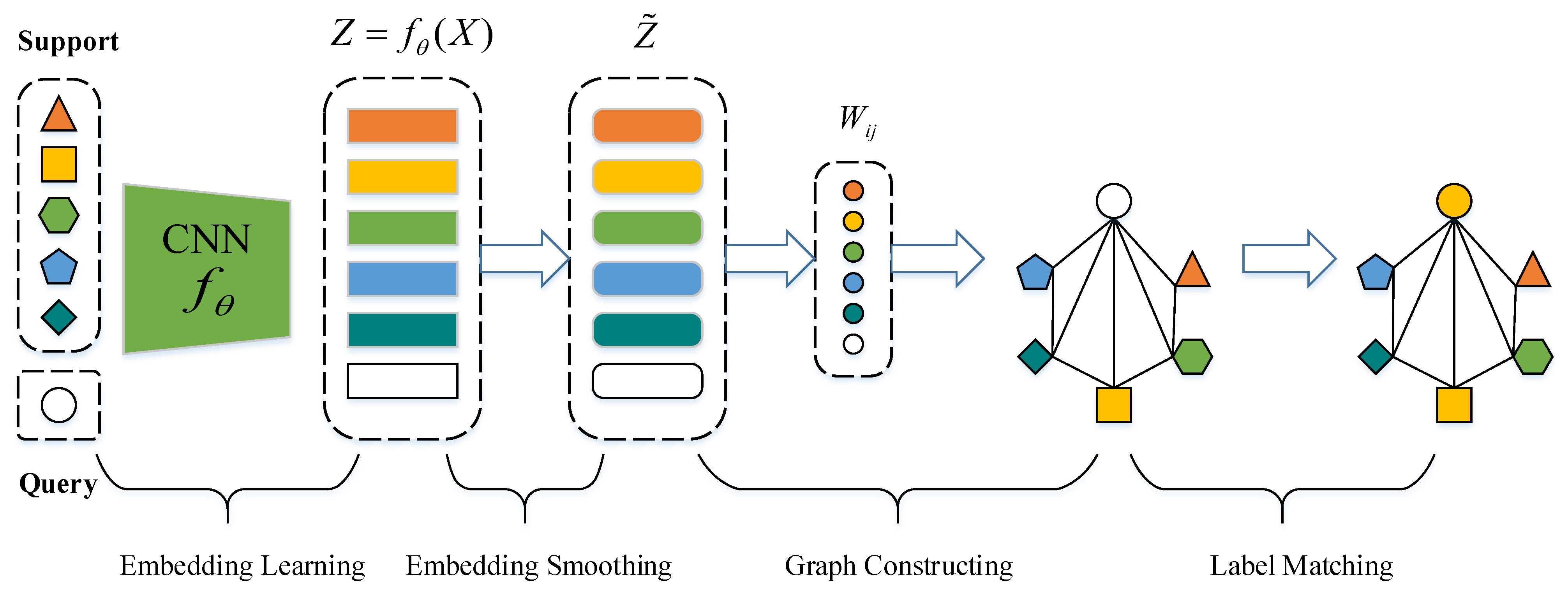
A novel graph neural network is presented for few-shot scene classification by transductive learning in this section, referred to as GES-Net. It is made up of four components: embedding learning, embedding smoothing, graph constructing, and label matching. As shown in Figure 2, GES-Net first extracts scene embedding features by a embedding learning module. Second, a new embedding smoothing method is presented to transform the embedding features into a cluster of interpolated features, which are referred to as smoothed embedding features. The smoothed embedding features are then adopted to calculate the task-level relation representation between nodes to carry out graph construction. Finally, given support samples, label matching is applied to label query samples on the constructed graph. On the one hand, GES-Net applies embedding smoothing to embedding features to enhance the smoothness of the embedding space by reducing various class-irrelevant noises, which was shown to improve generalization [16,17,18]. On the other hand, the proposed approach adopts the attention mechanism to measure task-level relation representation to perform graph constructing rather than common linear metrics.
3.1. Few-Shot Setting Setup
In our work, three datasets are given: a training set (), a test set (), and a validation set (). The training set was made up of a significant quantity of labeled data , where sample corresponds to category ∈. The test set , where derives from unseen category ∈ in the training set, that is ∩ = ∅, was adopted to estimate the generalization capability of the model. The validation set comprised the classes that do not exist in and and was adopted to adjust the hyperparameters.
Moreover, episode training was adopted to mimic the few-shot setting, that is an episode is referred to as a task. Each episode (task) is made up of N categories that are sampled uniformly without replacement from all categories, a support set S (K samples per category), and a query set Q (a total of T samples for all categories), which is termed N-way K-shot learning.
3.2. Embedding Learning
A CNN was employed to extract the embedding features of the input , where serves as the parameter of the network. By adopting the same backbone utilized in previous work [32,57,58], fair comparisons can be offered in the experiments, focusing on the effectiveness of the methods. The backbone contains four convolution modules, where each convolution module starts at a two-dimensional convolution layer containing a 3 × 3 convolution kernel and kernel size of 64. After each convolution layer, there is a batch normalization layer [45], a ReLU activation function [59], and a 2 × 2 max-pooling layer. The backbone is applied to the support set S and the query set Q.
3.3. Embedding Smoothing
Embedding smoothing is designed to process a set of embedding features that is obtained by inputting samples x of an episode into the embedding learning module . A group of new embedding features is then yielded by adopting the following steps. First, for the pairwise features (), the proposed approach calculates the distance as and the corresponding adjacent matrix as = exp , where is a scale parameter and for . was selected, which empirically made the training stage stable.
Next, the Laplacian of the adjacency matrix is calculated as,
where:
Subsequently, adopting the label propagation formulation described in [60], propagating matrix M is obtained as,
where denotes the scale parameter and I refers to the identity matrix. The smoothed embedding features are then yielded by the following operation,
Since is obtained by the weighted combination of its neighbors, embedding smoothing can effectively reduce the impact of noises from class-irrelevant features.
3.4. Graph Constructing
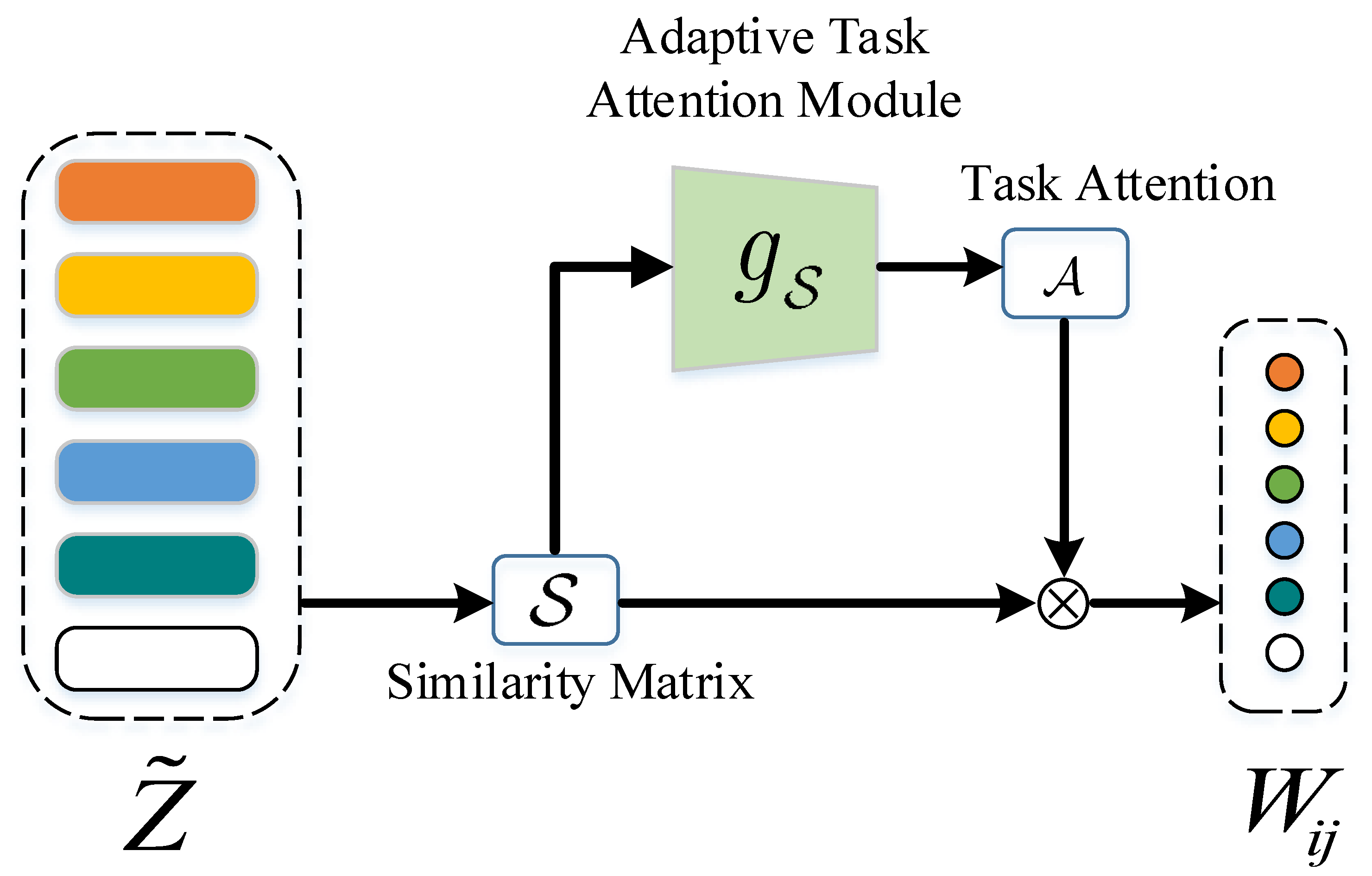
The embedded low-dimensional subspace in the data is uncovered by manifold learning, where selecting a suitable adjacency graph is crucial. To construct an appropriate adjacency graph in the few-shot setting, a novel graph constructing module is proposed, which was built around the attention mechanism. Specifically, the attention mechanism was adopted to convert smoothed embedding features to relation representations with regard to task-specific features; that is, the relation representation not only denotes the distance between nodes, but also contains the task-specific relation. The proposed graph constructing module can effectively avoid directly comparing irrelevant local relations. As shown in Figure 3, given smoothed embedding features , the task-level relation representation W can be achieved by Equation (7).
For node i, the corresponding attention value between the target embedding feature and features of all other samples in the task can be yielded by applying a common method in the attention mechanism. The corresponding attention value is acquired by the adaptive task attention module, which can be formulated as:
where represents the similarity degree of node i to node j and denotes the task-level similarity between nodes after comparing to all other nodes in the task. Therefore, the similarity degree between nodes is higher and is greater. The implementation of the similarity degree is obtained as follows:
where the smoothed embedding feature of the target sample is reshaped to adopting the matrix inversion operation and is the pairwise distance operation (e.g., radial basis function). Then, is employed to incorporate task-level information, and the relation representation for the current task can be acquired, which can be represented as follows:
The relation representation between node i and node j can be weighted through Equation (7), which denotes a task-level relation of node i to j after comparing to all the other nodes. While the relation representations of task-irrelevant regions are restrained, the relation representations of task-relevant regions are strengthened. To construct the k-nearest neighbor graph, the k-max values are reserved for each row of W. Then, the normalized graph Laplacian [61] is applied on W, that is,
where:
To simulate few-shot scenarios, the episodic paradigm for meta-training was followed; that is, the graph was separately constructed for each episode in each task, as shown in Figure 2. In general, in the setting of the five-way one-shot scenario, the shape of W is 80 × 80, which is quite efficient.
3.5. Label Matching
First, the prediction process of the labels of the query set Q is described. Assume represents the set of matrices, where each matrix is composed of nonnegative values and has a shape of . A label matrix is defined with if belongs to the support set and marked as , otherwise . Given the label matrix Y, label matching iteratively identifies the unseen labels of samples from on the constructed graph adopting the label propagation formula, i.e.,
where represents the inferred label matrix at the t-th round, L is the normalized graph weight, that is Equation (8), and weighs the amount of information from neighbors and Y. When t is large enough, there is a closed-form solution for the modified sequence,
where I denotes the identity matrix. Since this solution is directly applied to label prediction, the episodewise learning procedure becomes more effective.
Subsequently, the classification loss, between the predicted labels and the ground truth labels, is calculated. Specifically, to train all learnable parameters in an end-to-end manner, the cross-entropy loss was adopted in the experiments. Therein, ground truth labels derived from and the predicted scores were taken as corresponding inputs, where was transformed into prediction scores by the softmax function:
where is the ultimate predicted label for the i-th sample from and represents the j-th element of . Hence, the corresponding loss function can be written as:
where denotes the indicative function, that is = 0 if u is false and = 1 otherwise, and denotes the ground truth label corresponding to the sample . Note that, to imitate few-shot scenarios, all learnable parameters were iteratively updated by meta-learning in an end-to-end fashion.
4. Results and Discussion
In this section, our GES-Net approach is evaluated on three public remote sensing datasets for scene classification. The datasets used in the experiments are first described. The experimental settings and evaluation metrics are then illustrated in detail. Finally, the results of the experiments and analysis are presented.
4.1. Dataset Description
The validity of the proposed model was verified on three publicly available datasets, including UC Merced [62], WHU-RS19 [63], and NWPU-RESISC45 [64]. The dataset segmentation in [41] was followed, and the specific details are described below.
The UC Merced dataset contains 21 land use categories. There are 100 images in total per scene class, with a spatial resolution of 0.3 m. Each image consists of 256 × 256 pixels. In 2010, the dataset was released by the UC Merced Computer Vision Laboratory. In the dataset, 10 classes are split as the training set, 5 classes are deemed as the validation set, and 6 classes are selected as the test set.
The WHU-RS19 dataset is also a remote sensing scene dataset, which was released by Wuhan University. There are 19 diverse scene categories, and the image size of each category is at least 50 images. It includes a total of 1005 images with 600 × 600 pixels in size. For the dataset, 9 classes are split as the training set, 5 classes are divided as the validation set, and 5 classes are selected as the test set.
The NWPU-RESISC45 dataset is composed of 45 different classes in a total of 31,500 images. Each class consists of 700 images in the RGB color space. The pixel size per image is 256 × 256. In the dataset, the spatial resolution of most categories ranges from 0.2 m to 30 m for each pixel value. In the area of scene classification, NWPU-RESISC45 is the biggest in the matter of the total number of images and the quantity of the scene classes, which makes it abound with image variation, increasing classification difficulty. In our experiments, the dataset was split into 25, 10, and 10 categories as the training set, validation set, and test set, respectively.
4.2. Experimental Settings
For a fair comparison, four modules with the 3 × 3 convolution kernel and kernel size of 64 were selected for embedding learning. For each module, there was padding = 1 to retain abundant feature information, as well as the batch normalization layer [45], the ReLU nonlinearity activation function [59], as well as the 2 × 2 max pooling layer. The hyperparameter of embedding smoothing, of label matching, and k of the k-nearest neighbor graph were set to 0.5, 0.2, and 20, respectively, as suggested by Zhou et al. [60]. The proposed model was implemented in the PyTorch [65] framework, and the GPU was Tesla V100. Before training, all images are resized to 84 × 84 pixels. During the training period, the initial learning rate was set to 1 ×, and it was halved every 100 epochs. ADAM [66] was selected as the optimizer for our model.
4.3. Evaluation Metrics
For the performance evaluation, the proposed GES-Net approach was compared with the state-of-the-art approaches by the overall accuracy (OA) and confusion matrix (CM). OA is explicitly defined as:
where U denotes the number of tasks, that is the number of episodes, and is the number of samples that are rightly predicted in the j-th task. Specifically, the overall accuracy refers to the proportion of rightly classified query samples to the total quantity of query samples, that is the average of multiple episode results. In this work, all experimental results were averaged over 600 episodes by keeping the protocol in [57]. CM is an information table adopted to analyze the confusions and errors between various categories, where the item in the i-th row and j-th column refers to the proportion of test samples from the i-th category that are classified as the j-th category.
4.4. Time Complexity Analysis
In most scenarios, the overall accuracy is employed to evaluate the classification performance of deep neural networks. When practical issues need to be resolved, the time complexity required for the model should also be fully considered, which will significantly affect the cost of resolving the issues. For this purpose, floating-point operations (FLOPs) are typically adopted to estimate the time complexity of neural network models. For example, for the ResNet [67] series of networks, as the network depth continuously increases, the overall accuracy will also be improved, but it is noteworthy that the time and hardware costs will also rise significantly. Excessive parameters are liable to make model optimization more difficult, and it is hard to reach the anticipated classification effect.
When the classification effect of the model is relatively approximate, the model with a smaller time complexity is typically preferable. Therefore, the time complexity of various few-shot learning models on NWPU-RESISC45 in the setting of the five-way one-shot scenario is presented in Table 1. It can be seen that in the setting of the five-way one-shot scenario, the time complexity of our proposed approach was lower than that of RelationNet by 0.19 ×, and the classification accuracy exceeded RelationNet by at least 4.4%. Compared to other approaches, the approach we propose also achieved better results in terms of time complexity and classification accuracy. This is because only the embedding learning module contains learnable parameters, and other modules, such as embedding smoothing, graph constructing, and label matching, are non-parametric in our proposed framework. Therefore, our proposed model can achieve significant improvement at a relatively small cost.
4.5. Embedding Space Analysis
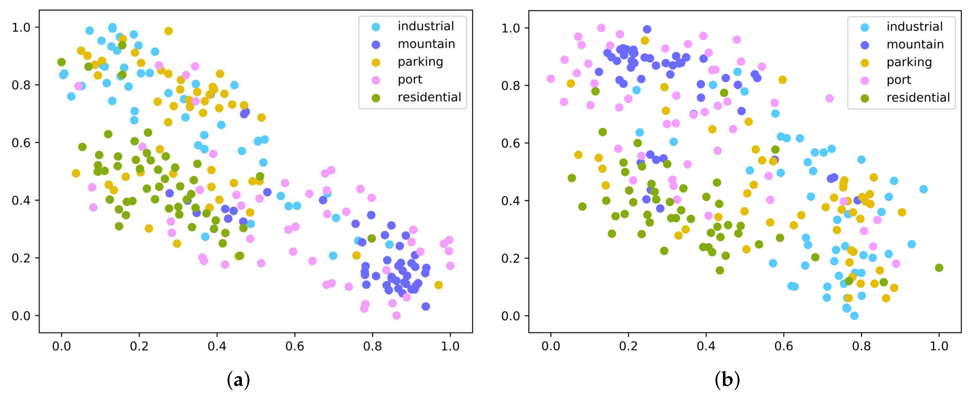
As indicated in Figure 1, the proposed method was carefully designed to solve the scene classification problem of only a few labeled samples and learn an embedding space that enables maximization of the gap between features of diverse categories and minimization of the gap between features of the same category to enhance the discrimination between sample features. Consequently, when there are unseen scene categories with one or five samples, scene classification can be achieved through the above idea. To verify this viewpoint, the five-way one-shot scenario was selected as the testing environment, and the test set was input into GES-Net and TPN [56]. TPN is one of the most influential few-shot learning approaches based on graph representation, which adopts label propagation to calculate label information for query samples. To illustrate the experimental results more intuitively, three subsets with five classes and one sample per class were individually sampled from the three datasets. T-SNE [68] was then adopted to visualize the experimental results on three datasets, namely UC Merced, WHU-RS19, and NWPU-RESISC45, as indicated in Figure 4, Figure 5 and Figure 6. It was noticed that the proposed GES-Net showed excellent results and was more discriminative than TPN in the embedding space, even though it had the phenomenon of separation between classes. Especially for the experiments on NWPU-RESISC45, the advantages of our GES-Net were more clearly shown; that is, samples belonging to diverse categories were more scattered and samples from the same category were more aggregated in the embedding space, which made the decision boundary more prominent. By comparison, samples from different categories embedded by the TPN algorithm were randomly distributed across the entire embedding space, and the decision boundaries among the diverse categories were quite blurred.
In addition, to measure the similarity degree between samples in the embedding space, Equation (6) was adopted in our proposed method. To illustrate the advantages of the metric we adopted, two commonly used metrics, that is the Euclidean distance and cosine distance, were utilized for comparison. Comparative experiments on NWPU-RESISC45 in the setting of the five-way one-shot scenario were carried out, as shown in Figure 7. It was observed that our proposed approach had a faster convergence rate, while obtaining higher classification performance as the number of iterations increased. Hence, the distance metric that we adopted was significantly superior to the more commonly used Euclidean distance and cosine distance.
4.6. Ablation Study
In this section, embedding smoothing and task-level relation representation are explored. Table 2 tabulates the experimental results obtained by ablating the embedding smoothing and task-level relation representation on the NWPU-RESISC45 dataset, where the following scenarios were considered.
4.6.1. Baseline
Embedding smoothing was excluded from the proposed model, and the task-level relation representation was replaced with the sample-level relation representation, that is TPN, which was implemented through the radial basis function.
4.6.2. Baseline+ES
Embedding smoothing was included in the proposed model, while task-level relation representation was not adopted.
4.6.3. Baseline+TR
The task-level relation representation was adopted, while embedding smoothing was not included.
From the experimental results, it was observed that combining the two components, namely embedding smoothing and task-level relation representation, could make our model achieve a superior classification performance. In the setting of the five-way one-shot scenario, the overall accuracies of Baseline+ES and Baseline+TR were 68.93% and 67.40%, respectively, higher than the Baseline, while in the setting of the five-way one-shot scenario, Baseline+ES obtained 81.73% overall accuracy, which was 3.23% higher than the Baseline. Moreover, in two scenarios, Baseline+ES achieved a higher overall accuracy than Baseline+TS, which indicates that ES (i.e., embedding smoothing) plays a more significant role in our model.
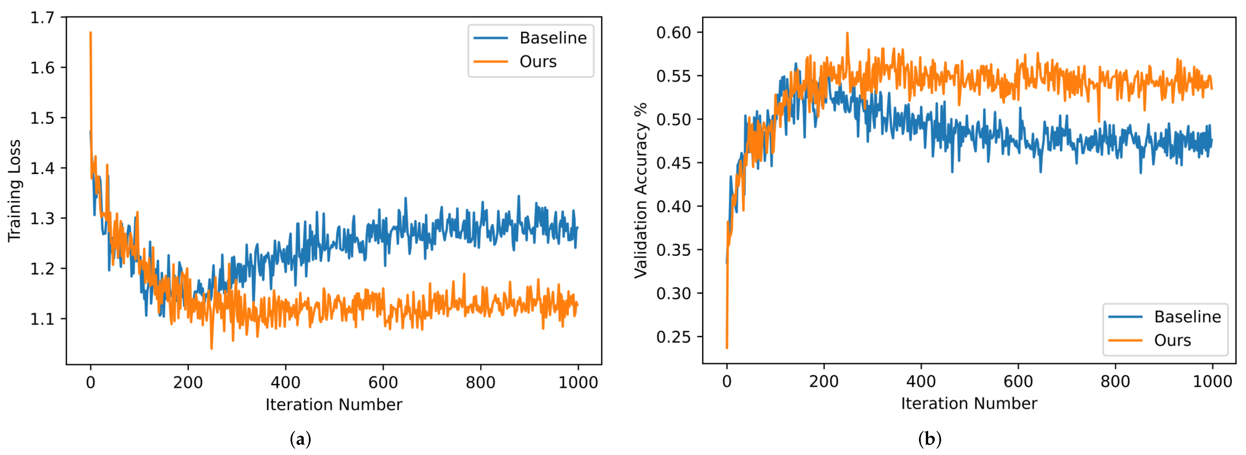
To further illustrate the effect of the above two components on the performance of the proposed GES-Net, five-way one-shot classification experiments were conducted on the NWPU-RESISC45 dataset. Figure 8 presents the specific experimental results, including the training loss and validation accuracy of our approach and the Baseline, that is TPN. The quantity of iterations was changed from 0–1000 with a step size of one. As can be observed in Figure 8, in the training stage, the training loss generated by our approach was smaller than that of the Baseline, and the highest validation accuracy achieved by our approach was greater than that of the Baseline. Moreover, to intuitively illustrate the advantages of the proposed embedding smoothing (ES), two commonly used regularization methods were compared with it, including spatial dropout (SD) and manifold mixup (MM). T-SNE was employed to visualize the experimental results of various regularization approaches on NWPU-RESISC45 in the five-way one-shot scenario, as shown in Figure 9, where the five colors correspond to the five scene categories. It was observed that the manifold of Baseline+ES was more concentrated and compact than Baseline+SD and Baseline+MM, which may reduce the impact of class-irrelevant noises on embedding representations.
Additionally, the experimental results were also measured in the confusion matrix. Figure 10 shows the confusion matrices for the three public datasets in the settings of the five-way one-shot and five-way five-shot scenarios. By comparing the left and right confusion matrices, it was observed that as the quantity of labeled samples per class increased, the confusion errors decreased and the accuracy of each class increased. This shows that as the quantity of labeled samples per class increased, the performance of our model also increased accordingly.
4.7. Comparison with the State-of-the-Art Approaches
To verify the validity of the proposed scheme, our proposed approach was compared with several recent approaches, including TPN [56], ProtoNet [57], MatchingNet [32], MAML [33], Meta-SGD [69], LLSR [14], RelationNet [58], RS-MetaNet [40], and DLA-MatchNet [41]. The experimental results of our approach and the above-mentioned approaches are shown in Table 3, Table 4 and Table 5, which consists of five-way one-shot and five-way five-shot results on three public benchmark datasets: UC Merced, WHU-RS19, and NWPU-RESISC45. All experiment results, presented in Table 3, Table 4 and Table 5, were averaged on 600 randomly sampled episodes in the test set. This shows that our proposed approach exceeded other approaches by a significant margin and obtained state-of-the-art results on the three public benchmark datasets. Even though our proposed approach slightly surpassed RS-MetaNet in the five-way one-shot scenario on UC Merced, it exceeded RS-MetaNet by at least 5.58% in other scenarios. Overall, our proposed approach showed great superiority in multiple scenarios, e.g., 1-shot (1.65%) on UC Merced, 1-shot (7.57%) and 5-shot (1.67%) on WHU-RS19, and 1-shot (2.03%) on NWPU-RESISC45.
5. Conclusions
A novel graph neural network framework, referred to as GES-Net, was presented for the few-shot scene classification of remote sensing images in this paper. GES-Net regularizes the embedding space through a non-parametric embedding smoothing strategy. Embedding smoothing can constrain the embedding features, which enables the embedding learning module to extract more discriminative and robust scene embedding features to deal with complex and realistic scenarios. Moreover, GES-Net adopts an attention mechanism to capture the task-level relation representation. Considering the embedding features of all samples in a task, our method can obtain the task-level relation representation between nodes to construct the graph. Comparative experiments on three remote sensing scene datasets remarkably demonstrated the validity of GES-Net and outperformed state-of-the-art approaches by a considerable margin. Additionally, several ablation studies were conducted to analyze the influence of embedding smoothing and the task-level relation representation. However, there is still a great deal of unlabeled remote sensing data that are not utilized in the real world. Therefore, in future work, a large amount of unlabeled data will be introduced into the training procedure of the model to further improve the performance of scene classification in the settings of finite labeled samples.
Author Contributions
Conceptualization, Z.Y., W.H., C.T. and X.L.; methodology, W.H., A.Y. and C.T.; software, Z.Y. and A.Y.; validation, Z.Y., W.H. and C.T.; formal analysis, C.T.; resources, Z.Y. and X.L.; investigation, X.L.; data curation, C.T. and X.L.; writing—original draft preparation, Z.Y. and W.H.; writing—review and editing, W.H. and A.Y.; supervision, Z.Y. and C.T.; visualization, Z.Y. and W.H.; funding acquisition, X.L.; project administration, W.H. and C.T. All authors have read and agreed to the published version of the manuscript.
Funding
This work was supported by the National Natural Science Foundation of China (Grant No. 41871226).
Institutional Review Board Statement
Not applicable.
Informed Consent Statement
Not applicable.
Data Availability Statement
The data provided in this work are available from the corresponding author.
Conflicts of Interest
The authors declare no conflict of interest.
References
- Zhao, B.; Zhong, Y.; Xia, G.S.; Zhang, L. Dirichlet-derived multiple topic scene classification model for high spatial resolution remote sensing imagery. IEEE Trans. Geosci. Remote Sens. 2015, 54, 2108–2123. [Google Scholar] [CrossRef]
- Yao, X.; Han, J.; Cheng, G.; Qian, X.; Guo, L. Semantic annotation of high-resolution satellite images via weakly supervised learning. IEEE Trans. Geosci. Remote Sens. 2016, 54, 3660–3671. [Google Scholar] [CrossRef]
- Huang, X.; Wang, Y. Investigating the effects of 3D urban morphology on the surface urban heat island effect in urban functional zones by using high-resolution remote sensing data: A case study of Wuhan, Central China. ISPRS J. Photogramm. Remote Sens. 2019, 152, 119–131. [Google Scholar] [CrossRef]
- Zhao, W.; Du, S. Learning multiscale and deep representations for classifying remotely sensed imagery. ISPRS J. Photogramm. Remote Sens. 2016, 113, 155–165. [Google Scholar] [CrossRef]
- Huang, X.; Han, X.; Ma, S.; Lin, T.; Gong, J. Monitoring ecosystem service change in the City of Shenzhen by the use of high-resolution remotely sensed imagery and deep learning. Land Degrad. Dev. 2019, 30, 1490–1501. [Google Scholar] [CrossRef]
- Zhu, Q.; Zhong, Y.; Zhang, L.; Li, D. Adaptive deep sparse semantic modeling framework for high spatial resolution image scene classification. IEEE Trans. Geosci. Remote Sens. 2018, 56, 6180–6195. [Google Scholar] [CrossRef]
- Wu, Z.; Li, Y.; Plaza, A.; Li, J.; Xiao, F.; Wei, Z. Parallel and distributed dimensionality reduction of hyperspectral data on cloud computing architectures. IEEE J. Sel. Top. Appl. Earth Obs. Remote Sens. 2016, 9, 2270–2278. [Google Scholar] [CrossRef]
- Chen, J.; Wang, C.; Ma, Z.; Chen, J.; He, D.; Ackland, S. Remote sensing scene classification based on convolutional neural networks pre-trained using attention-guided sparse filters. Remote Sens. 2018, 10, 290. [Google Scholar] [CrossRef] [Green Version]
- Zhu, Q.; Zhong, Y.; Wu, S.; Zhang, L.; Li, D. Scene classification based on the sparse homogeneous–heterogeneous topic feature model. IEEE Trans. Geosci. Remote Sens. 2018, 56, 2689–2703. [Google Scholar] [CrossRef]
- Liu, Y.; Zhong, Y.; Qin, Q. Scene classification based on multiscale convolutional neural network. IEEE Trans. Geosci. Remote Sens. 2018, 56, 7109–7121. [Google Scholar] [CrossRef] [Green Version]
- Zhao, B.; Huang, B.; Zhong, Y. Transfer learning with fully pretrained deep convolution networks for land-use classification. IEEE Geosci. Remote Sens. Lett. 2017, 14, 1436–1440. [Google Scholar] [CrossRef]
- Gidaris, S.; Bursuc, A.; Komodakis, N.; Pérez, P.; Cord, M. Boosting few-shot visual learning with self-supervision. In Proceedings of the 2019 IEEE/CVF International Conference on Computer Vision, ICCV 2019, Seoul, Korea, 27 October–2 November 2019; pp. 8059–8068. [Google Scholar]
- Chu, W.H.; Li, Y.J.; Chang, J.C.; Wang, Y.C.F. Spot and learn: A maximum-entropy patch sampler for few-shot image classification. In Proceedings of the IEEE/CVF Conference on Computer Vision and Pattern Recognition, Long Beach, CA, USA, 16–20 June 2019; pp. 6251–6260. [Google Scholar]
- Zhai, M.; Liu, H.; Sun, F. Lifelong learning for scene recognition in remote sensing images. IEEE Geosci. Remote Sens. Lett. 2019, 16, 1472–1476. [Google Scholar] [CrossRef]
- Garcia, V.; Bruna, J. Few-shot learning with graph neural networks. In Proceedings of the 6th International Conference on Learning Representations, ICLR 2018, Vancouver, BC, Canada, 30 April–3 May 2018; pp. 1–13. [Google Scholar]
- Bartlett, P.; Shawe-Taylor, J. Generalization performance of support vector machines and other pattern classifiers. In Advances in Kernel Methods: Support Vector Learning; MIT Press: Cambridge, MA, USA, 1999; pp. 43–54. [Google Scholar]
- Lee, W.S.; Bartlett, P.L.; Williamson, R.C. Lower bounds on the VC dimension of smoothly parameterized function classes. Neural Comput. 1995, 7, 1040–1053. [Google Scholar] [CrossRef]
- Verma, V.; Lamb, A.; Beckham, C.; Najafi, A.; Mitliagkas, I.; Lopez-Paz, D.; Bengio, Y. Manifold mixup: Better representations by interpolating hidden states. In Proceedings of the 36th International Conference on Machine Learning (PMLR), Long Beach, CA, USA, 9–15 June 2019; pp. 6438–6447. [Google Scholar]
- Wang, S.; Wang, X.; Zhang, L.; Zhong, Y. Auto-AD: Autonomous Hyperspectral Anomaly Detection Network Based on Fully Convolutional Autoencoder. IEEE Trans. Geosci. Remote Sens. 2021, 60, 1–4. [Google Scholar] [CrossRef]
- Zhan, T.; Song, B.; Xu, Y.; Wan, M.; Wang, X.; Yang, G.; Wu, Z. SSCNN-S: A Spectral-Spatial Convolution Neural Network with Siamese Architecture for Change Detection. Remote Sens. 2021, 13, 895. [Google Scholar] [CrossRef]
- Wang, Y.; Hou, J.; Hou, X.; Chau, L.P. A Self-Training Approach for Point-Supervised Object Detection and Counting in Crowds. IEEE Trans. Image Process. 2021, 30, 2876–2887. [Google Scholar] [CrossRef] [PubMed]
- Zhu, S.; Du, B.; Zhang, L.; Li, X. Attention-Based Multiscale Residual Adaptation Network for Cross-Scene Classification. IEEE Trans. Geosci. Remote Sens. 2021, 60. [Google Scholar] [CrossRef]
- Chen, J.; Qiu, X.; Ding, C.; Wu, Y. CVCMFF Net: Complex-Valued Convolutional and Multifeature Fusion Network for Building Semantic Segmentation of InSAR Images. IEEE Trans. Geosci. Remote Sens. 2021, 60. [Google Scholar] [CrossRef]
- Xu, C.; Zhu, G.; Shu, J. A Lightweight and Robust Lie Group-Convolutional Neural Networks Joint Representation for Remote Sensing Scene Classification. IEEE Trans. Geosci. Remote Sens. 2021, 60. [Google Scholar] [CrossRef]
- Wang, X.; Wang, S.; Ning, C.; Zhou, H. Enhanced Feature Pyramid Network With Deep Semantic Embedding for Remote Sensing Scene Classification. IEEE Trans. Geosci. Remote Sens. 2021, 59, 7918–7932. [Google Scholar] [CrossRef]
- Penatti, O.A.; Nogueira, K.; Dos Santos, J.A. Do deep features generalize from everyday objects to remote sensing and aerial scenes domains? In Proceedings of the 2015 IEEE Conference on Computer Vision and Pattern Recognition Workshops (CVPRW), Boston, MA, USA, 7–12 June 2015; pp. 44–51. [Google Scholar]
- Lu, X.; Zheng, X.; Yuan, Y. Remote sensing scene classification by unsupervised representation learning. IEEE Trans. Geosci. Remote Sens. 2017, 55, 5148–5157. [Google Scholar] [CrossRef]
- Lu, X.; Gong, T.; Zheng, X. Multisource compensation network for remote sensing cross-domain scene classification. IEEE Trans. Geosci. Remote Sens. 2019, 58, 2504–2515. [Google Scholar] [CrossRef]
- Lu, X.; Sun, H.; Zheng, X. A feature aggregation convolutional neural network for remote sensing scene classification. IEEE Trans. Geosci. Remote Sens. 2019, 57, 7894–7906. [Google Scholar] [CrossRef]
- Nogueira, K.; Penatti, O.A.; Dos Santos, J.A. Towards better exploiting convolutional neural networks for remote sensing scene classification. Pattern Recognit. 2017, 61, 539–556. [Google Scholar] [CrossRef] [Green Version]
- Cheng, G.; Yang, C.; Yao, X.; Guo, L.; Han, J. When deep learning meets metric learning: Remote sensing image scene classification via learning discriminative CNNs. IEEE Trans. Geosci. Remote Sens. 2018, 56, 2811–2821. [Google Scholar] [CrossRef]
- Vinyals, O.; Blundell, C.; Lillicrap, T.; Kavukcuoglu, K.; Wierstra, D. Matching Networks for One Shot Learning. Proc. Neural Inf. Process. Syst. 2016, 29, 3630–3638. [Google Scholar]
- Finn, C.; Abbeel, P.; Levine, S. Model-agnostic meta-learning for fast adaptation of deep networks. In Proceedings of the International Conference on Machine Learning PMLR, Sydney, Australia, 6–11 August 2017; pp. 1126–1135. [Google Scholar]
- Santoro, A.; Bartunov, S.; Botvinick, M.; Wierstra, D.; Lillicrap, T. Meta-learning with memory-augmented neural networks. In Proceedings of the International Conference on Machine Learning PMLR, New York, NY, USA, 19–24 June 2016; pp. 1842–1850. [Google Scholar]
- Tokmakov, P.; Wang, Y.X.; Hebert, M. Learning compositional representations for few-shot recognition. In Proceedings of the IEEE/CVF International Conference on Computer Vision (ICCV), Seoul, Korea, 27 October–2 November 2019; pp. 6372–6381. [Google Scholar]
- Li, H.; Dong, W.; Mei, X.; Ma, C.; Huang, F.; Hu, B.G. Lgm-net: Learning to generate matching networks for few-shot learning. In Proceedings of the International Conference on Machine Learning PMLR, Long Beach, CA, USA, 9–15 June 2019; pp. 3825–3834. [Google Scholar]
- Liu, B.; Yu, X.; Yu, A.; Zhang, P.; Wan, G.; Wang, R. Deep few-shot learning for hyperspectral image classification. IEEE Trans. Geosci. Remote Sens. 2018, 57, 2290–2304. [Google Scholar] [CrossRef]
- Gao, K.; Liu, B.; Yu, X.; Qin, J.; Zhang, P.; Tan, X. Deep relation network for hyperspectral image few-shot classification. Remote Sens. 2020, 12, 923. [Google Scholar] [CrossRef] [Green Version]
- Rostami, M.; Kolouri, S.; Eaton, E.; Kim, K. Deep transfer learning for few-shot sar image classification. Remote Sens. 2019, 11, 1374. [Google Scholar] [CrossRef] [Green Version]
- Li, H.; Cui, Z.; Zhu, Z.; Chen, L.; Zhu, J.; Huang, H.; Tao, C. RS-MetaNet: Deep Metametric Learning for Few-Shot Remote Sensing Scene Classification. IEEE Trans. Geosci. Remote Sens. 2020, 59, 6983–6994. [Google Scholar] [CrossRef]
- Li, L.; Han, J.; Yao, X.; Cheng, G.; Guo, L. DLA-MatchNet for Few-Shot Remote Sensing Image Scene Classification. IEEE Trans. Geosci. Remote Sens. 2020, 59, 7844–7853. [Google Scholar] [CrossRef]
- Guo, Y.; Codella, N.C.; Karlinsky, L.; Codella, J.V.; Smith, J.R.; Saenko, K.; Rosing, T.; Feris, R. A broader study of cross-domain few-shot learning. In European Conference on Computer Vision; Vedaldi, A., Bischof, H., Brox, T., Frahm, J.M., Eds.; Springer: Cham, Switzerland, 2020; pp. 124–141. [Google Scholar]
- Gong, T.; Zheng, X.; Lu, X. Cross-Domain Scene Classification by Integrating Multiple Incomplete Sources. IEEE Trans. Geosci. Remote Sens. 2020, 59, 10035–10046. [Google Scholar] [CrossRef]
- Yosinski, J.; Clune, J.; Bengio, Y.; Lipson, H. How transferable are features in deep neural networks? Proc. Adv. Neural Inf. Process. Syst. 2014, 27, 3320–3328. [Google Scholar]
- Ioffe, S.; Szegedy, C. Batch normalization: Accelerating deep network training by reducing internal covariate shift. In Proceedings of the International Conference on Machine Learning PMLR, Lille, France, 6–11 July 2015; pp. 448–456. [Google Scholar]
- Srivastava, N.; Hinton, G.; Krizhevsky, A.; Sutskever, I.; Salakhutdinov, R. Dropout: A simple way to prevent neural networks from overfitting. J. Mach. Learn. Res. 2014, 15, 1929–1958. [Google Scholar]
- Tompson, J.; Goroshin, R.; Jain, A.; LeCun, Y.; Bregler, C. Efficient object localization using convolutional networks. In Proceedings of the IEEE Conference on Computer Vision and Pattern Recognition, Boston, MA, USA, 7–12 June 2015; pp. 648–656. [Google Scholar]
- Rodríguez, P.; Gonzalez, J.; Cucurull, G.; Gonfaus, J.M.; Roca, X. Regularizing cnns with locally constrained decorrelations. arXiv 2016, arXiv:1611.01967. [Google Scholar]
- Salimans, T.; Kingma, D.P. Weight normalization: A simple reparameterization to accelerate training of deep neural networks. Proc. Adv. Neural Inf. Process. Syst. 2016, 29, 901–909. [Google Scholar]
- Zhang, H.; Cisse, M.; Dauphin, Y.N.; Lopez-Paz, D. mixup: Beyond empirical risk minimization. arXiv 2017, arXiv:1710.09412. [Google Scholar]
- Belkin, M.; Niyogi, P.; Sindhwani, V. Manifold regularization: A geometric framework for learning from labeled and unlabeled examples. J. Mach. Learn. Res. 2006, 7, 2399–2434. [Google Scholar]
- Cho, K.; Zhao, J. Retrieval-augmented convolutional neural networks against adversarial examples. In Proceedings of the IEEE/CVF Conference on Computer Vision and Pattern Recognition (CVPR), Long Beach, CA, USA, 16–20 June 2019; pp. 11563–11571. [Google Scholar]
- Vapnik, V.N. An overview of statistical learning theory. IEEE Trans. Neural Netw. 1999, 10, 988–999. [Google Scholar] [CrossRef] [PubMed] [Green Version]
- Iscen, A.; Tolias, G.; Avrithis, Y.; Chum, O. Label propagation for deep semi-supervised learning. In Proceedings of the IEEE/CVF Conference on Computer Vision and Pattern Recognition (CVPR), Long Beach, CA, USA, 16–20 June 2019; pp. 5070–5079. [Google Scholar]
- Liu, B.; Wu, Z.; Hu, H.; Lin, S. Deep metric transfer for label propagation with limited annotated data. In Proceedings of the 2019 IEEE/CVF International Conference on Computer Vision Workshops, ICCV Workshops 2019, Seoul, Korea, 27–28 October 2019; pp. 1–10. [Google Scholar]
- Liu, Y.; Lee, J.; Park, M.; Kim, S.; Yang, E.; Hwang, S.J.; Yang, Y. Learning to propagate labels: Transductive propagation network for few-shot learning. arXiv 2018, arXiv:1805.10002. [Google Scholar]
- Snell, J.; Swersky, K.; Zemel, R. Prototypical networks for few-shot learning. In Proceedings of the Advances in Neural Information Processing Systems, Long Beach, CA, USA, 4–9 December 2017; pp. 4080–4090. [Google Scholar]
- Sung, F.; Yang, Y.; Zhang, L.; Xiang, T.; Torr, P.H.; Hospedales, T.M. Learning to compare: Relation network for few-shot learning. In Proceedings of the IEEE/CVF Conference on Computer Vision and Pattern Recognition, Salt Lake City, UT, USA, 18–22 June 2018; pp. 1199–1208. [Google Scholar]
- Glorot, X.; Bordes, A.; Bengio, Y. Deep sparse rectifier neural networks. In Proceedings of the International Conference Artificial Intelligence and Statistics, JMLR Workshop and Conference Proceedings, Fort Lauderdale, FL, USA, 11–13 April 2011; pp. 315–323. [Google Scholar]
- Zhou, D.; Bousquet, O.; Lal, T.N.; Weston, J.; Schölkopf, B. Learning with local and global consistency. In Proceedings of the Advances in Neural Information Processing Systems, Vancouver, BC, Canada, 13–18 December 2004; pp. 321–328. [Google Scholar]
- Chung, F.R.; Graham, F.C. Spectral Graph Theory; Number 92; AMS, American Mathematical Society: Providence, RI, USA, 1997. [Google Scholar]
- Yang, Y.; Newsam, S. Bag-of-visual-words and spatial extensions for land-use classification. In Proceedings of the 18th ACM SIGSPATIAL International Conference on Advances in Geographic Information Systems (ACM SIGSPATIAL GIS 2010), San Jose, CA, USA, 2–5 November 2010; pp. 270–279. [Google Scholar]
- Sheng, G.; Yang, W.; Xu, T.; Sun, H. High-resolution satellite scene classification using a sparse coding based multiple feature combination. Int. J. Remote Sens. 2012, 33, 2395–2412. [Google Scholar] [CrossRef]
- Cheng, G.; Han, J.; Lu, X. Remote sensing image scene classification: Benchmark and state of the art. Proc. IEEE 2017, 105, 1865–1883. [Google Scholar] [CrossRef] [Green Version]
- Paszke, A.; Gross, S.; Chintala, S.; Chanan, G.; Yang, E.; DeVito, Z.; Lin, Z.; Desmaison, A.; Antiga, L.; Lerer, A. Automatic differentiation in pytorch. In Proceedings of the Workshop Advances Neural Information Processing Systems, Long Beach, CA, USA, 4–9 December 2017; pp. 1–4. [Google Scholar]
- Kingma, D.P.; Ba, J. Adam: A Method for Stochastic Optimization. In Proceedings of the 3rd International Conference for Learning Representations, San Diego, CA, USA, 7–9 May 2015. [Google Scholar]
- He, K.; Zhang, X.; Ren, S.; Sun, J. Deep residual learning for image recognition. In Proceedings of the IEEE/CVF Conference on Computer Vision and Pattern Recognition (CVPR), Honolulu, HI, USA, 21–26 July 2016; pp. 770–778. [Google Scholar]
- Van der Maaten, L.; Hinton, G. Visualizing data using t-SNE. J. Mach. Learn. Res. 2008, 9, 2579–2605. [Google Scholar]
- Li, Z.; Zhou, F.; Chen, F.; Li, H. Meta-sgd: Learning to learn quickly for few-shot learning. arXiv 2017, arXiv:1707.09835. [Google Scholar]
Figure 1.
Illustration of adopting few-shot learning to learn scene information from only two labeled images.
Figure 1.
Illustration of adopting few-shot learning to learn scene information from only two labeled images.

Figure 2.
Graph-based embedding smoothing network framework for the 5-way 1-shot scenario with one query sample.
Figure 2.
Graph-based embedding smoothing network framework for the 5-way 1-shot scenario with one query sample.

Figure 3.
Schematic of the task-level relation module.

Figure 4.
Embedding feature visualization of GES-Net (a) and TPN (b) on UC Merced in the 5-way 1-shot scenario.
Figure 4.
Embedding feature visualization of GES-Net (a) and TPN (b) on UC Merced in the 5-way 1-shot scenario.

Figure 5.
Embedding feature visualization of GES-Net (a) and TPN (b) on WHU-RS19 in the 5-way 1-shot scenario.
Figure 5.
Embedding feature visualization of GES-Net (a) and TPN (b) on WHU-RS19 in the 5-way 1-shot scenario.

Figure 6.
Embedding feature visualization of GES-Net (a) and TPN (b) on NWPU-RESISC45 in the 5-way 1-shot scenario.
Figure 6.
Embedding feature visualization of GES-Net (a) and TPN (b) on NWPU-RESISC45 in the 5-way 1-shot scenario.

Figure 7.
Validation accuracies with diverse distance metrics on the NWPU-RESISC45 dataset in the setting of the 5-way 1-shot scenario.
Figure 7.
Validation accuracies with diverse distance metrics on the NWPU-RESISC45 dataset in the setting of the 5-way 1-shot scenario.

Figure 8.
Training loss and validation accuracy on the NWPU-RESISC45 dataset in the setting of the 5-way 1-shot scenario. The training loss is shown on the left, and the validation accuracy is shown on the right. (a) Training loss; (b) validation accuracy.
Figure 8.
Training loss and validation accuracy on the NWPU-RESISC45 dataset in the setting of the 5-way 1-shot scenario. The training loss is shown on the left, and the validation accuracy is shown on the right. (a) Training loss; (b) validation accuracy.

Figure 9.
Visualization of embedding features with different regularization approaches on the same dataset.
Figure 9.
Visualization of embedding features with different regularization approaches on the same dataset.

Figure 10.
Confusion matrices on UC Merced (top), WHU-RS19 (middle), and NWPU-RESISC45 (bottom). The experiment results with only one sample per class (one-shot) are shown on the left, and those with five samples per class (five-shot) are shown on the right. (a) One-shot on UC Merced; (b) five-shot on UC Merced; (c) one-shot on WHU-RS19; (d) five-shot on WHU-RS19; (e) one-shot on NWPU-RESISC45; (f) five-shot on NWPU-RESISC45.


Table 1.
Time complexity analysis of different approaches on NWPU-RESISC45 in the same few-shot setting (%).
Table 1.
Time complexity analysis of different approaches on NWPU-RESISC45 in the same few-shot setting (%).
| Method | 5-Way 1-Shot Accuracy | FLOPs |
|---|---|---|
| ProtoNet | 40.33 ± 0.18 | |
| MatchingNet | 37.61 | |
| MAML | 48.40 ± 0.82 | |
| RelationNet | 66.43 ± 0.73 | |
| GES-Net (ours) | 70.83 ± 0.85 |
Table 2.
Ablation study of embedding smoothing (ES) and task-level relation (TR). The comparison experiments were conducted on NWPU-RESISC45 (%).
Table 2.
Ablation study of embedding smoothing (ES) and task-level relation (TR). The comparison experiments were conducted on NWPU-RESISC45 (%).
| Model | 5-Way | |
|---|---|---|
| 1-Shot | 5-Shot | |
| Baseline | 66.51 ± 0.87 | 78.50 ± 0.56 |
| Baseline+ES | 68.93 ± 0.91 | 81.73 ± 0.59 |
| Baseline+TR | 67.40 ± 0.85 | 80.93 ± 0.61 |
| GES-Net (ours) | 70.83 ± 0.85 | 82.27 ± 0.55 |
Table 3.
Few-shot overall accuracies and standard deviations (%) on UC Merced.
| Model | 5-Way | |
|---|---|---|
| 1-Shot | 5-Shot | |
| TPN | 53.36 ± 0.77 | 68.23 ± 0.52 |
| ProtoNet | 52.27 ± 0.20 | 69.86 ± 0.15 |
| MatchingNet | 34.70 | 52.71 |
| MAML | 48.86 ± 0.74 | 60.78 ± 0.62 |
| Meta-SGD | 50.52 ± 2.61 | 60.82 ± 2.00 |
| LLSR | 39.47 | 57.40 |
| RelationNet | 48.08 ± 1.67 | 61.88 ± 0.50 |
| RS-MetaNet | 57.23 ± 0.56 | 76.08 ± 0.28 |
| DLA-MatchNet | 53.76 ± 0.60 | 63.01 ± 0.51 |
| GES-Net (ours) | 58.88 ± 0.81 | 81.66 ± 0.50 |
Table 4.
Few-shot overall accuracies and standard deviations (%) on WHU-RS19.
| Model | 5-Way | |
|---|---|---|
| 1-Shot | 5-Shot | |
| TPN | 59.28 ± 0.72 | 71.20 ± 0.55 |
| ProtoNet | 58.01 ± 0.16 | 80.70 ± 0.11 |
| MatchingNet | 50.13 | 54.10 |
| MAML | 49.13 ± 0.65 | 62.49 ± 0.51 |
| Meta-SGD | 51.54 ± 2.31 | 61.74 ± 2.02 |
| LLSR | 57.10 | 70.65 |
| RelationNet | 60.92 ± 1.86 | 79.75 ± 1.19 |
| DLA-MatchNet | 68.27 ± 1.83 | 79.89 ± 0.33 |
| GES-Net (ours) | 75.84 ± 0.78 | 82.37 ± 0.38 |
Table 5.
Few-shot overall accuracies and standard deviations (%) on NWPU-RESISC45.
| Model | 5-Way | |
|---|---|---|
| 1-Shot | 5-Shot | |
| TPN | 66.51 ± 0.87 | 78.50 ± 0.56 |
| ProtoNet | 40.33 ± 0.18 | 63.82 ± 0.56 |
| MatchingNet | 37.61 | 47.10 |
| MAML | 48.40 ± 0.82 | 62.90 ± 0.69 |
| Meta-SGD | 60.63 ± 0.90 | 75.75 ± 0.65 |
| LLSR | 51.43 | 72.90 |
| RelationNet | 66.43 ± 0.73 | 78.35 ± 0.51 |
| RS-MetaNet | 52.78 ± 0.09 | 71.49 ± 0.81 |
| DLA-MatchNet | 68.80 ± 0.70 | 81.63 ± 0.46 |
| GES-Net (ours) | 70.83 ± 0.85 | 82.27 ± 0.55 |
Publisher’s Note: MDPI stays neutral with regard to jurisdictional claims in published maps and institutional affiliations. |
© 2022 by the authors. Licensee MDPI, Basel, Switzerland. This article is an open access article distributed under the terms and conditions of the Creative Commons Attribution (CC BY) license (https://creativecommons.org/licenses/by/4.0/).
Share and Cite
MDPI and ACS Style
Yuan, Z.; Huang, W.; Tang, C.; Yang, A.; Luo, X. Graph-Based Embedding Smoothing Network for Few-Shot Scene Classification of Remote Sensing Images. Remote Sens. 2022, 14, 1161. https://doi.org/10.3390/rs14051161
AMA Style
Yuan Z, Huang W, Tang C, Yang A, Luo X. Graph-Based Embedding Smoothing Network for Few-Shot Scene Classification of Remote Sensing Images. Remote Sensing. 2022; 14(5):1161. https://doi.org/10.3390/rs14051161
Chicago/Turabian StyleYuan, Zhengwu, Wendong Huang, Chan Tang, Aixia Yang, and Xiaobo Luo. 2022. "Graph-Based Embedding Smoothing Network for Few-Shot Scene Classification of Remote Sensing Images" Remote Sensing 14, no. 5: 1161. https://doi.org/10.3390/rs14051161
Note that from the first issue of 2016, this journal uses article numbers instead of page numbers. See further details here.