Abstract
In the increasingly complex electromagnetic environment, a variety of new signal types are appearing; however, existing electromagnetic signal classification (ESC) models cannot handle new signal types. In this context, the emergence of class-incremental learning aims to incrementally update the classification model as new categories emerge. In this paper, an electromagnetic signal classification framework based on class exemplar selection and a multi-objective linear programming classifier (CES-MOLPC) is proposed in order to continuously learn new classes in an incremental manner. Specifically, our approach involves the adaptive selection of class exemplars considering normalized mutual information and a multi-objective linear programming classifier. The former is used to maintain the classification capability of the model for previous categories by selecting key samples, while the latter is used to allow the model to adapt quickly to new categories. Meanwhile, a weighted loss function based on cross-entropy and distillation loss is presented in order to fine-tune the model. We demonstrate the effectiveness of the proposed CES-MOLPC method through extensive experiments on the public RML2016.04c data set and the large-scale real-world ACARS signal data set. The results of the comparative experiments demonstrate that our method can achieve significant improvements over state-of-the-art methods.
1. Introduction
Electromagnetic signal classification (ESC) is a key technology in the field of information processing, which forms the basis for non-cooperative communications [1], electronic counter-measures [2], smart antennas [3], software radio [4], and wireless spectrum management [5]. With the widespread use of various types of radio equipment, the types and numbers of radiation sources in the electromagnetic environment are increasing, and the electromagnetic spectrum is becoming more and more congested. More importantly, electromagnetic signal data are acquired faster than before. Under these circumstances, electromagnetic signal data have applications in many fields, such as electromagnetic spectrum monitoring [6], cognitive radio [7], and cyberspace security [8]. ESC is an important requirement for these applications. ESC includes electromagnetic signal type classification and specific emitter identification (SEI). The main task of the former is to exploit the characteristics of electromagnetic signals to distinguish different signal types [8], while the latter involves measuring the characteristics of the received electromagnetic signals and determining the individual radiation sources that generate the signals, based on available prior information [9].
Existing methods based on deep learning have recently achieved remarkable success in the field of signal classification. Many correlative algorithms [10,11] have been proposed and have achieved excellent classification results. For instance, in [12], a graph convolutional modulation recognition framework has been proposed to identify the modulation type of the signal. In [13], a framework based on the capsule network has been proposed to solve the small sample modulation-type detection problem. In [14], a sequence-based network has been proposed. In [15], a convolutional neural network for radio modulation classification has been presented, which is not only suitable for the complex time domain of radio signals but also can achieve excellent results under low signal-to-noise ratio (SNR) conditions. A residual neural network [16] has been used in [17] to perform signal classification over a range of configurations and channel impairments, providing reliable statistics. To solve the task of modulation signal classification, AlexNet and GoogleNet have been used in [18] and achieved great results, proving the effectiveness of deep learning methods in this area. In [10], the authors proposed a complex-valued convolutional neural network, which was used to study the intrinsic properties of the radar interference signal. The authors in [19] have developed a small sample signal modulation recognition framework using an attention relation network. In [20], a convolutional long short-term deep neural network has been used to fully exploit the temporal properties of electromagnetic signals and achieve excellent performance. In [21], a multitasking-based generalized automatic modulation classification framework has been proposed, which was more robust than conventional methods. Moreover, in [22], the authors proved the effectiveness of a deep model in identifying interference sources using frequency band, SNR, and sample selection to optimize the training time. A generative adversarial network has been proposed, in [8], to address the problem of insufficiently labeled electromagnetic signal samples.
Although researchers have conducted many explorations on deep learning-based ESC methods and achieved good results, there is a pre-condition for such deep learning algorithms, which is that the number of signal categories that these algorithms can recognize is fixed. When multiple new categories appear, a natural approach to incremental learning is to simply fine-tune a pre-trained model with the training data of new categories. However, a serious challenge to this approach is catastrophic forgetting [23]; specifically, fine-tuning a model on new data usually results in a significant drop in performance on previous categories. The model has to be trained with the training data of all the previously observed categories in order to recognize the new and the old classes simultaneously. This leads to high computational effort and memory requirements.
With the increasing number of signal processing tasks, electromagnetic signal data have shown an explosive growth trend. In particular, we are faced with the constant emergence of new categories of electromagnetic signal data. For example, in the field of coded communication and adaptive modulation, the receiver recognizes the coding and the modulation method used by the transmitter, and then uses the corresponding decoding and demodulation algorithm to decode and demodulate the acquired signal. When the transmitter changes the modulation mode, the signal received by the receiver will be a new class. When managing the spectrum, cognitive radio can monitor whether illegal signals are interfering with the user’s communications by detecting radio signals in the perceived frequency band. If there are multiple categories of illegal signals, they should be identified immediately. Moreover, in realistic applications, new categories are expected to keep appearing over time. If the classification accuracy on the previous categories of the classification model decreases after the learning task of the new class is completed at each stage, there will theoretically be an infinite number of new classes to learn, thus creating an infinite loop.
Class incremental learning is a suitable learning mode for this scenario, where the data increase gradually. Class-incremental learning algorithms can learn a set of gradually evolving classification tasks, and the categories in each task have no overlap with the categories in other tasks. In recent years, driven by practical applications, class incremental learning has gradually become an important research topic. Existing deep learning-based algorithms can be mainly divided into the following three categories: regularization-based, rehearsal-based, and bias-correction-based. The core idea of regularization-based approaches is to estimate the importance of each parameter in the network [23]. The regularization element was added, in [24,25], in order to penalize parameters that vary widely. To constrain important parameters, ref. [26] have introduced regularization terms in the loss function. Furthermore, the authors of [27] have attempted to use the idea of data regularization to prevent activation drift. MAS [28] uses the gradient of the loss function to measure the importance of neurons. The work in [29] preserved old knowledge by freezing the weights of the last layer and penalizing differences between activations before the classification layer. Rehearsal-based methods can mitigate the catastrophic forgetting phenomenon by storing a small number of old samples [30,31], or using a generation network to generate fake samples [32,33]. In [30], the distillation loss and an exemplar set of old categories were used to train the model for the first time. In [34], a semantic drift compensation algorithm was used to estimate the center of each category and perform the prediction by the NCM classifier [30]. In [35], a supervised contrast loss was used to bring samples from the same category closer together in the embedding space, while samples of different classes were further apart in the embedding space. Bias-correction-based methods are dedicated to addressing the problem of imbalance between new and old tasks [31,36,37]. To alleviate such an imbalance, cosine normalization, less-forget constraint, and inter-class separation have been proposed in [36]. To address the problem that the norm of the classifier weight vector of new categories is larger than that of old categories, the weight aligning [37] method has been proposed, which cooperates better with the distillation loss. Another effective algorithm has been proposed in [31], which corrects the biases of different tasks by adding an additional linear layer.
In real ESC applications, an incremental learning algorithm may be able to use part of the previous samples. What an incremental learning method based on the class exemplar selection should do is retain the previous classification capabilities in the form of exemplars of the old categories. The samples selected by the rehearsal-based methods described above can only maintain the classification performance of the model for samples in the center of the class. In order to maintain the classification ability of the model for samples far from the class center at the same time, more efficient samples should be selected. Many exemplar selection-based strategies have recently been proposed [38]. They can be broadly divided into two categories: model output-based and training data distribution-based. Model output-based methods use some output indicators of the classification model as the exemplar selection criteria. In [39], samples were selected based on the lowest confidence level, but the sample set selected in this way was redundant. In [40], the output probability of the model was used as the selection criterion. The entropy-based method was proposed in [41]. Studies have also considered the prediction of errors [42] and interface-distance-based sampling [23]. Training data distribution-based methods use the characteristics of the data itself as the selection criterion. In [30], the average feature vector was extracted. Then, selection was performed according to the distance between the feature vector of each sample and the center of the class feature. In [43], clustering information was used to select the effective samples. Some samples were randomly selected from the whole data set as exemplars. In general, methods based on random sampling are used for comparison with other methods [23,44]. However, the samples selected by the abovementioned methods can only represent the class very well, while discrimination between classes is not sufficient for the models to achieve good classification results for old classes.
It is not an easy task to develop a good classification model which is suitable for new classes. The model must be able to classify new classes while maintaining its ability to recognize old categories. Nevertheless, existing deep learning approaches are not suitable for the above situations. In summary, the challenges facing ESC can be expressed as follows:
- (1)
- How to maintain the classification performance of the model when new categories of electromagnetic signal data emerge. As the number of different electromagnetic devices increases and the amount of collected signal data continues to grow, various new types of signals may be mixed with the existing data. Furthermore, data are updated rapidly, making it an unrealistic task to save all signal data for further training when memory is limited. The emergence of multiple categories and the updating of large data require the deep model to rapidly update its classification capabilities; however, existing state-of-the-art deep learning approaches are not able to learn new categories efficiently; and
- (2)
- How to maintain the model’s ability to classify old classes after learning the new class. A model trained on old categories may suffer from catastrophic forgetting [23] after learning new categories. If all of the data from the previously observed classes are used to train the new model, significant computational overhead and time costs will be incurred. Mainstream methods based on exemplar selection are usually based on prototypes [30]. These methods use the mean value of the extracted features as the selection criterion. However, samples selected in this way can only represent the class very well, while discrimination between classes is not sufficient for the model to achieve good classification results on the old classes.
To overcome the aforementioned problems, we present a multi-class incremental learning framework, CES-MOLPC, for ESC, which not only can learn new classes rapidly but also ensures that its classification accuracy on old classes is maintained at a high value. Specifically, we develop a multi-objective linear programming (MOLP) incremental classifier based on the average feature vectors extracted by the deep extractor. Inspired by [45], the proposed MOLP classifier is obtained by solving the MOLP problem, where the whole process only requires forward propagation of the old model without using a back-propagation algorithm to train the model. In addition, inspired by [46,47,48], we develop an adaptive class exemplar selection approach, in view of the normalized mutual information, in order to maintain the accuracy of new model on previous categories. We also design a weighted loss function based on cross-entropy and distillation loss, which is used to fine-tune the incremental model, thus making the model more robust. The presented method requires only a small amount of computational and storage resources. In summary, the main innovative contributions of this article are as follows:
- (1)
- The presented MOLP classifier learns multiple new categories simultaneously by increasing multiple weight vectors, which can be obtained by solving the MOLP problem based on the average feature vector of each class;
- (2)
- The presented adaptive class exemplar selection approach, in view of normalized mutual information, preserves the classification ability of the model for previous categories by selecting key samples; and
- (3)
- A weighted loss function based on cross-entropy and distillation loss is presented to fine-tune the new model using both the new category data and the old exemplar set.
The remainder of this article is organized as follows: in Section 2, the proposed ESIC framework is presented. Section 3 shows the numerical examples to verify the classification performance of our method. In Section 4, we discuss the proposed method and experimental results. Finally, in Section 5, we summarize the main results of this paper.
2. Methodology
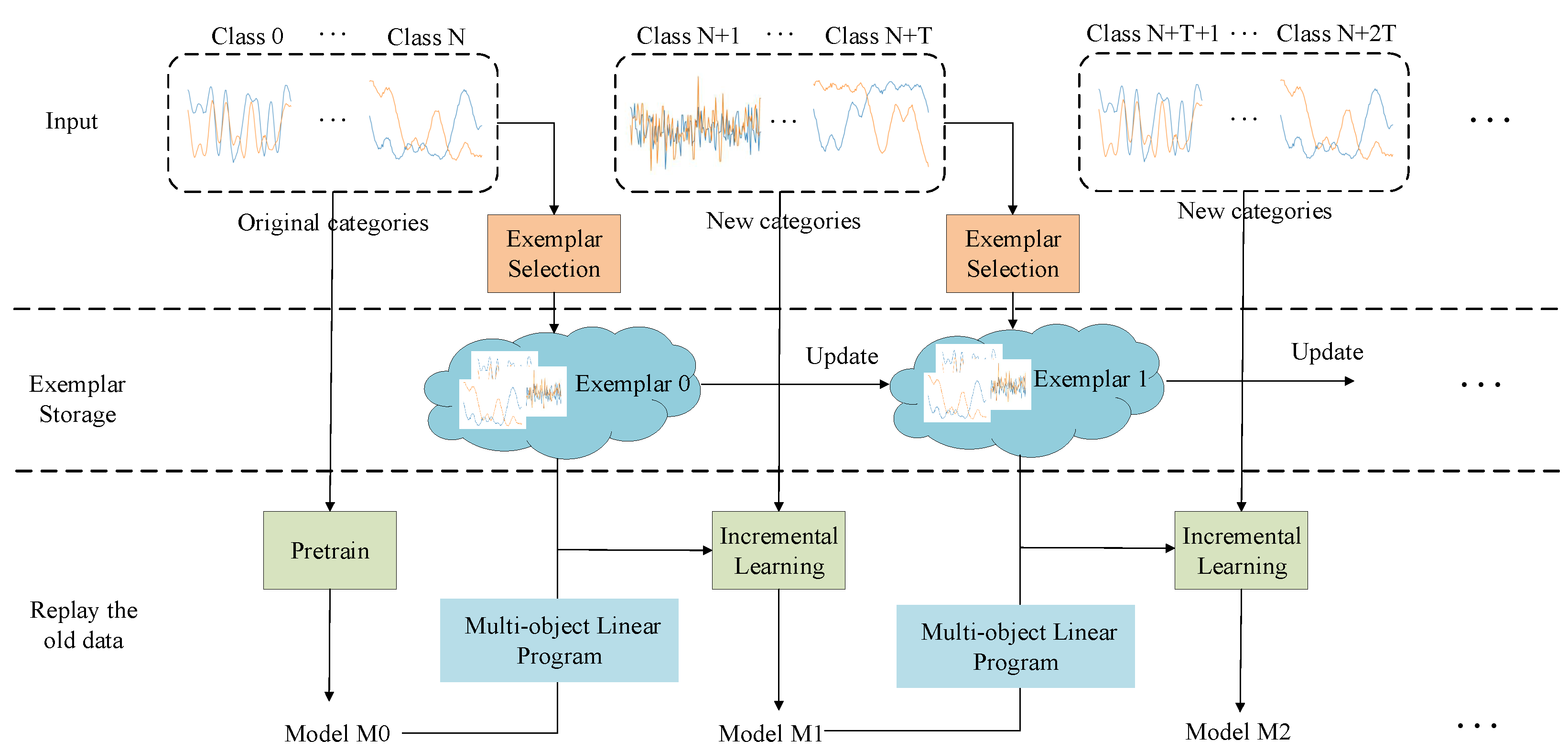
According to the electromagnetic signal increment classification (ESIC) framework, shown in Figure 1, the proposed framework is mainly composed of the following three modules:
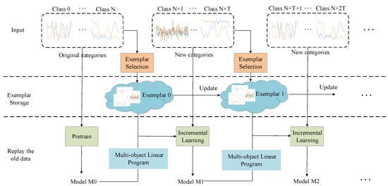
Figure 1.
Overview of the proposed framework, CES-MOLPC.
- (1)
- Adaptive class exemplar selection;
- (2)
- MOLP incremental classifier; and
- (3)
- Incremental learning.
The specific description, with respect to the proposed algorithm, is given in the following. Assuming that there are N categories of signal data, a model trained using these data has the ability to accurately classify N old categories, where is a feature extractor, is an N-class classifier, and is the weight matrix of the classifier. In our model, the bias of the classifier is set to 0. In the ESIC task, the signal data constantly appear in a stream. In the case of limited memory size, only a small part of the training data can be saved. Therefore, the exemplar selection approach, in view of normalized mutual information, is presented for the selection of key samples. When T unknown categories are used as input to the model, the model must correctly identify the N old categories while also being able to identify the T new categories well. At this time, the output layer of the model must add T output nodes; that is, the weight matrix of the classifier needs to add T weight columns. Thus, the MOLP classifier is proposed to learn new classes by adding T weight columns. is obtained by solving the MOLP problem. Finally, in the incremental learning stage, the exemplars of the old classes and the data of the new class are fused to fine-tune the model . At the same time, cross-entropy loss and distillation loss are adopted for fine-tuning. Our goal is to obtain the incremental model .
2.1. Adaptive Exemplar Selection
The idea behind the proposed exemplar selection approach is to calculate the normalized mutual information between the one-hot vector corresponding to the true label of the sample and the probability vector predicted by model for the sample. The one-hot vector and the class vector predicted by the model for the sample can be regarded as two clusters, where the resemblance between the two clusters is measured by the normalized mutual information. We assume that the harder a sample is to identify as belonging to the correct category, the closer it is to the decision boundary. Specifically, on the premise that a sample is correctly classified, if there is less normalized mutual information between the ground-truth label and the probability of the sample predicted by model, the more difficult it is for the sample to be recognized as the correct category, which means that we can select a small number of boundary samples to describe the sample distribution of the entire category.
As shown in Algorithm 1, given the data of N old categories , the exemplar is selected from . An initial model, , is trained to recognize N classes using all data from . When T new classes appear, they are integrated with the exemplars of old categories to train a new model. The normalized mutual information between the one-hot ground-truth label and predicted label is shown in (1).
where refers to the mutual information between and , as shown in (2); refers to the entropy of , as shown in (3); and refers to the entropy of , as shown in (4).
| Algorithm 1 Adaptive class exemplar selection |
|
Previous algorithms based on sample playback select the same number of samples in each category. In this work, an adaptive exemplar selection method, which is weighted based on the number of samples, is proposed to maintain the classification ability on old categories. As the classification difficulty for each category is different, it is not necessary for each category to preserve the same number of samples. For the categories that are difficult to distinguish, more samples should be retained, while samples that are easy to distinguish need only retain a small number of samples. When selecting the exemplar set, the recognition accuracy of the old model on the old training data is used as feedback. If the recognition rate for a certain old category is higher, then fewer samples should be saved, accordingly. In addition, the degree of dispersion of the category distribution is also used as a measure. We use the mean value of the distance between the feature vector of all samples in a category and the average feature vector to measure the distribution of samples in the category. The more concentrated the sample distribution of the category, the higher the similarity within the category, such that fewer samples are required to describe the category. The weight factor is shown in (5):
where is the classification accuracy on the class, refers to the number of training samples in the class, refers to the feature vector of the sample, and refers to the average feature vector of the class.
As the memory size is fixed, considering the number of samples in each category and then normalizing the weights of all old categories to between 0 and 1, the number of samples that need to be saved for each category can be obtained, as shown in (6):
where represents the number of samples that need to be saved in the signal data of the first type in the old data.
2.2. MOLP Incremental Classifier
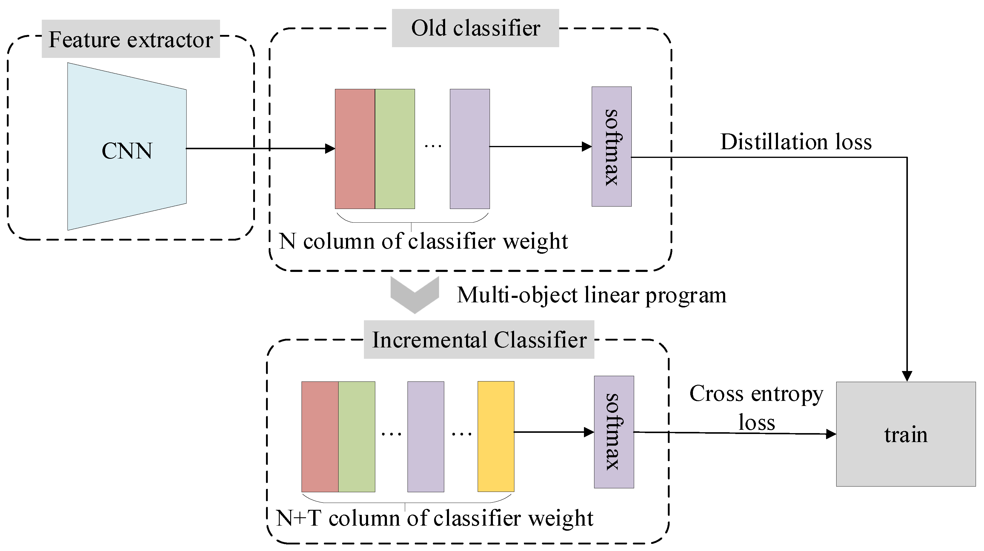
As shown in Figure 2, when the model needs to learn T new categories, the classifier must add T output nodes; that is, the weight matrix needs to add T columns. According to the classification principle of the linear classifier, when the new category data are input to the CNN model, the feature vector is first extracted through the feature extractor, following which the feature is used as input to the linear classification layer to obtain a vector. Each component in the vector denotes the possibility that the sample belongs to certain category. Thus, the component value corresponding to the new class should be maximized.
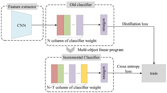
Figure 2.
MOLP incremental classifier and training of the model.
Given the model trained on old categories and a sample x of the category, as well as the eigenvector f of x extracted by the feature extractor , the existing classifier gives the score by classifier dot multiplying f with . Then, the softmax activation function is used to obtain the probability of x belonging to the category, as shown in (7):
where , is dimensional, as shown in (8); refers to the column of the weight matrix; and L refers to the dimension of the eigenvector. When T new categories arrive, the new classifier corresponds to the weight matrix , as shown in (9):
The exemplar set of old categories and new categories of data are used as input to the model. The class mean eigenvector of each class is obtained by averaging each eigenvector extracted by the sophisticated extractor :
where refers to the mean feature vector of old categories, and refers to the mean feature vector of new categories at a time. When the mean feature vector of the old category is input to the classification layer, it will predict a score by multiplying the class feature vector by the new weight matrix, as shown in (11). should be maximized in ; thus, we can formulate it as , , , which leads to the constraint of the MOLP problem.
If the feature vector of the new category is input into the classifier, it will predict a score by multiplying the class feature vector with the new weight matrix, as shown in (12). should be maximized in ; thus, we can formulate it as , , , , which leads to the constraint of the MOLP problem. We take as the maximization goal of the MOLP.
In summary, we can express the MOLP problem as follows:
where is the mean feature vector of the new category, is the mean feature vector of the old category, denotes the column of the new weight matrix, denotes the column of the new weight matrix, and denotes the largest value of the old weight matrix. By solving the above MOLP problem, we can obtain the new classifier .
2.3. Incremental Learning
After completing the exemplar selection of old classes and obtaining the incremental classifier , the last step is incremental learning. The specific algorithm flow is detailed in Algorithm 2. The old exemplar set and data of new categories are integrated to fine-tune the model . In the incremental learning phase, both the cross-entropy loss and distillation loss are used when fine-tuning the new incremental model. The cross-entropy loss is designed to guide the model to better distinguish signal categories, while distillation loss is used to help the new model not forget the knowledge of the old model as much as possible. Our loss function can be expressed as follows:
where is equal to , N is the number of old classes, and T is the number of new classes. The standard cross-entropy loss and the distillation loss are as follows:
where collects the old exemplar set and all the data of the new classes, is the indicator function, is the probability that the input signal belongs to the category obtained by the new model, is the soft label of the input signal generated by old model on all observed categories and y is the ground-truth label, and is a rescaling function, where is scaling factor ( in our experiments) which increases the weights of small values.
| Algorithm 2 Incremental learning |
|
3. Results
3.1. Data Set
To test the effectiveness of the presented framework for signal classification (CES-MOLPC), we performed comparative experiments on both the public RML2016.04c data set and the large-scale real-world ACARS signal data set.
The signal-to-noise ratio of the RML2016.04c dataset ranges from −20 to 18 dB, with an interval of 2 dB. The corresponding in-phase and quadrature signal (IQ) for each signal-to-noise ratio includes 11 modulation types, of which 8 are digital modulations and the remaining 3 are analog modulations. We used the 12 dB data as the experimental data set. The total number of training samples was 8103, but the numbers of samples for each category differed. The dimensions of each signal sample were .
As a digital data transmission system, ACARS is generally used to transmit messages between aircraft and ground stations by radio or satellite. At present, ACARS is used in many civil aviation systems. The data set in this article was collected using our own experimental system, whose antenna was placed at a specific place in Jiaxing, Zhejiang Province, China. There were 10,000 ACARS signals from 20 aircraft overall, such that the data set had a total of 20 categories, with each category containing 500 samples. In our experiment, the training samples and test samples each accounted for half of the samples. The dimensions of each IQ signal sample were .
3.2. Experimental Setup
3.2.1. Parameters
In the following experiment, the memory size was limited to 200, the Adam optimizer was used when fine-tuning the model, the learning rate was set to 0.001 throughout the training of the old classes and the fine-tuning phases, the weight decay was 0.00001 in the whole process, the batch size in the whole process was 32, and the number of iterations was 500 for the training of the old classes and 80 for the fine-tuning phase.
3.2.2. Network Structure
We created two convolutional neural networks for incremental classification on the above two data sets. The network structure corresponding to the RML2016.04c data set is given in Table 1, which mainly consisted of three convolutional layers, three pooling layers, and three regularization layers. A dropout layer was used to reduce overfitting. The network structure corresponding to the ACARS data set is shown in Table 2. This network mainly consisted of seven convolutional layers, seven pooling layers, and seven regularization layers.

Table 1.
The neural network structure (RML2016.04c).
Table 2.
The neural network structure (ACARS).
3.2.3. Evaluation Metrics
We defined the evaluation metrics Old OA, New OA, and Total OA, where New OA refers to the ratio of the number of correctly classified samples in the test samples of all the new classes to the total number of test samples in the new class; Old OA refers to the ratio of the number of correctly classified samples in all the test samples of the old class to the total number of test samples in the old class; and Total OA refers to the ratio of the number of correctly classified samples in the test samples of all the categories to the total number of test samples in all the categories.
3.2.4. Environment
Our experiment was conducted on a computer with an Inter(R) Xeon(R) Gold 6240 CPU with 128 GB RAM at 2.60 GHz and an NVIDIA GeForce RTX 3090 GPU with 24 GB RAM. The software environment was the Ubuntu 16.04 64 bit system, and the deep learning frameworks of PyTorch were used.
3.3. Result and Analysis of Experiments
3.3.1. Multi-Class Recognition Performance
To validate the advantages of our presented overall framework, CES-MOLPC, we performed multi-class recognition experiments and compared the results with those of several competing or representative methods, including Incremental Classifier and Representation Learning (ICARL) [30], Bias Correction (BIC) [31], and Weight Aligning (WA) [37]. These methods all use a portion of the old class signal samples to maintain the incremental model’s ability to classify the old classes after learning a new class. To ensure the fairness of the experiment, the size of the exemplar set of our approach matched that used in the above approaches, and the network structure and hyper-parameters of the comparison methods were also consistent with those of our method. The experiments considering all of the abovementioned methods were performed five times, and the average value was taken as the final result.
For the RML2016.04c data set, we set the number of new categories to 1, 2, or 3 (T = 1, 2, 3). Table 3 shows the experimental results on the RML2016.04c data set. When , the proposed approach (CES-MOLPC) achieved the highest values of Old OA and Total OA, while the difference in New OA between our method and the best was only 0.26. The WA method does not learn any new knowledge at all, and its New OA was not as high as that of our method. In contrast, the BIC method is biased towards new classes. The possible reason for this is that the weighted loss function is not balanced. The ICARL method performed worse than the BIC method. When , the CES-MOLPC method also achieved the best Old OA and Total OA, but its New OA value was low. Meanwhile, the BIC method had the best New OA, but it obviously forgot the old knowledge. The Total OA of our method was 0.3 higher than that of the second-highest method. When , CES-MOLPC performed best on old categories. The OA of the second-best method, WA, was only 0.21 lower than our method, but its New OA was poor. The BIC approach was still biased towards new classes. In the above three cases, CES-MOLPC achieved the highest Total OA. Obviously, the proposed method achieved the best classification results, when compared to the other methods.
Table 3.
Results of experiments on the RML2016.04c data set ().
For the ACARS data set, we set the number of new categories to 2, 4, or 6 (T = 2, 4, 6). Table 4 shows the experimental results on the ACARS data set. When , the proposed approach, CES-MOLPC, achieved the best Old OA and New OA, and its Total OA was 2% higher than that of the runner-up. The Old OA value of the WA method was only 0.04% lower than that of the proposed method, but its New OA was very poor. When , CES-MOLPC had the highest New OA and Total OA, while the Old OA of the proposed method was lower than that of WA; however, the New OA value of WA is only 0.59%, which means that the method had basically not learned the knowledge of the new classes at all. This is probably due to this method scaling the weights of the new classifiers too much, such that the new classifiers tend too much to the old classes. When , CES-MOLPC performed best for the overall category. The ICARL method had the highest New OA, while the WA method had the highest Old OA. In the above three cases, the proposed CES-MOLPC outperformed all of the compared methods, in terms of the Total OA. This means that our approach was more robust.
Table 4.
Results of experiments on the ACARS data set ().
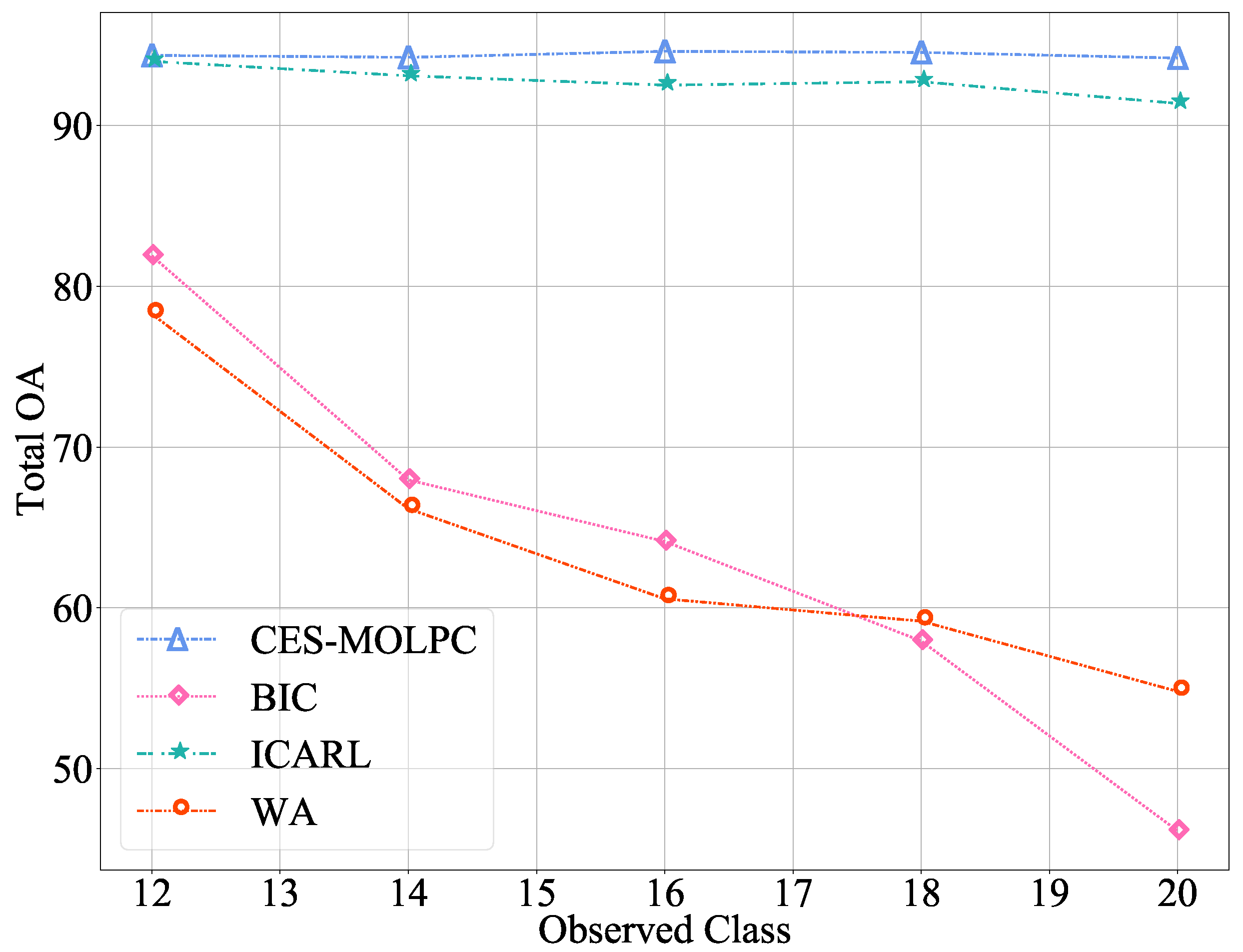
In order to further observe the effectiveness of our method in alleviating catastrophic forgetting problems, we set up several continuous incremental processes. For the RML2016.04c data set, set the number of old classes to 5 and the number of new classes to 6, adding one class each time. For the ACARS data set, we set the number of old and new categories to 10, and added two categories each time. The experimental results are shown in Figure 3 and Figure 4. The abscissa in the figure represents the number of classes learned by the model, and the ordinate represents the classification accuracy of the current model on the test data of all learned classes.
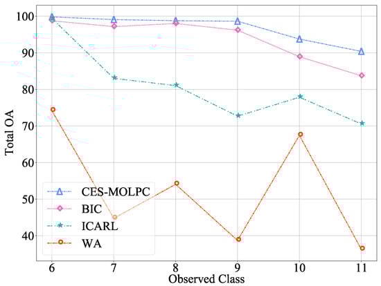
Figure 3.
The Total OA of multiple incremental classification on the RML2016.04c data set ().
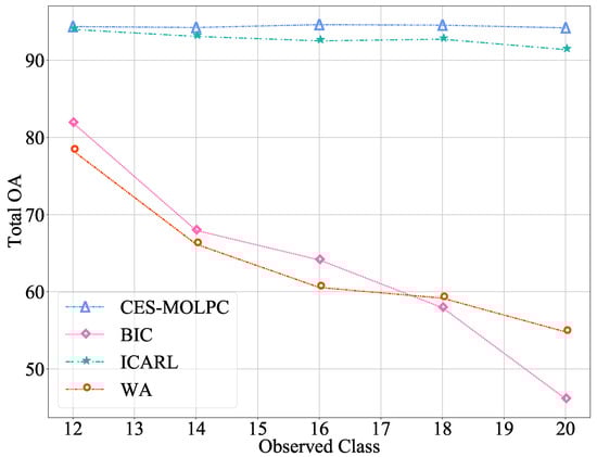
Figure 4.
The Total OA of multiple incremental classification on the ACARS data set ().
From the figures, we can observe the advantages of our proposed CES-MOLPC: the accuracy of this method decreased very slowly in all the categories. The BIC method performed well on the RML2016.04c data set, but it was still not as good as our method. When the number of categories learned was 9, the decrease was even more significant. The ICARL method performed well on the ACARS data set, but was second to our method. The WA method performed poorly on both data sets, with significant variation and low accuracy. It can be seen that our proposed method was not only effective in learning new categories, but also retained the classification ability of the model for old categories.
3.3.2. Comparison to Other Class Exemplar Selection Methods
To determine the additional benefits of class exemplar selection, we compared the proposed CES-MOLPC with other class exemplar selection approaches. The other algorithms included Random, Entropy [41], and Prototype [30]. The Random method randomly selects old exemplars from the old data. The Prototype approach selects the signal samples whose feature vectors are close to the average feature vector of its own category. All experiments were performed five times and the average was taken as the final result.
Table 5 shows the comparative experimental results of the class exemplar selection methods on the RML2016.04c data set. It can be seen that the proposed CES-MOLPC achieved the highest classification accuracy. The Entropy exemplar selection method performed better than the Prototype method. Both Old OA and Total OA of the Random method outperformed the other two methods, and were only slightly behind those of our method. The New OA of these methods was low, mainly as the old classes contained similar categories to the new classes. Table 6 lists the comparative experimental results of class exemplar selection methods on the ACARS data set. We can see that the presented method achieved the highest classification accuracy in all three indicators (i.e., Old OA, New OA, and Total OA). As the Prototype method only considers representativeness when selecting samples but ignores the distinction between classes, the Old OA of this method was not as good as that of the Entropy and Random methods.
Table 5.
Comparison of class exemplar selection methods on the RML2016.04c data set ().
Table 6.
Comparison of class exemplar selection methods on the ACARS data set ().
4. Discussion
In terms of computational complexity, the proposed algorithms mainly included multi-objective linear programming, adaptive class example selection, and incremental learning. The interior-point method was used to solve linear programming problems, such that the time complexity was . During the process of adaptive class exemplar selection, the normalized mutual information of each sample and the Euclidean distance between each sample and its class feature center had to be computed, and so its computational complexity was . During the process of incremental learning, the deep model was fine-tuned. Therefore, we introduce the concept of floating point operations (FLOPs) to illustrate the computational complexity. The FLOPs of the model corresponding to the RML2016.04c data set were 1.28 M, while the FLOPs of the model corresponding to the ACARS data set were 2.83 M.
To further illustrate the computational complexity of the proposed method, we performed a comparative experiment considering the runtime of the algorithm, setting on both the RML2016.04c data set and the ACARS data set. Table 7 and Table 8 show the running times of the proposed method and other comparable methods for learning new classes. We can see that the running time of the proposed CES-MOLPC was much shorter than those of the other methods. The proposed method, CES-MOLPC, took only 1.64 min to complete learning of a new class on the RML2016.04c data set; however, that on the ACARS data set took a longer time, due to the high dimensionality of the data. Taken together, the other methods took more than three times as much time as the proposed method, CES-MOLPC.
Table 7.
Algorithm running time comparison on RML2016.04c data set ().
Table 8.
Algorithm running time comparison on ACARS data set ().
From the experimental results shown in Table 3 and Table 4, the proposed method showed good generalization performance for the public data set RML2016.04c, as well as for the signal data set ACARS recorded in a real environment. The Total OA corresponding to the proposed method surpassed that of other comparison methods; however, the New OA and Old OA values were different. In fact, as the distillation loss was used to fine-tune the model, it was difficult for New OA and Old OA to reach a relatively balanced condition simultaneously. We privately performed a more extreme experiment, in order to adjust the ratio of cross-entropy loss and distillation loss. When the cross-entropy loss was much larger than the distillation loss, the resulting New OA was higher and the Old OA was lower. Meanwhile, if the distillation loss was much greater than the cross-entropy loss, then New OA would be higher and Old OA would be lower. In the WA method, it was assumed that the L2-norms of the weight vectors of the classifiers corresponding to the new and old classes were different, such that the weight alignment method was used to balance the new and old classes, for which distillation loss was also used. However, in the experimental results, the Old OA corresponding to the WA method was almost 0 in any case and, so, this method is not suitable for the problem considered in this paper. Therefore, the advantages of the proposed method can be seen from the experimental results. In incremental learning, both the Old OA and the New OA must be considered. Taken together, the proposed method outperformed the comparison methods. The common feature of the BIC, ICARL, and WA methods was that they all used the Prototype exemplar selection method. From Table 5 and Table 6, it can be seen that the adaptive sample selection method based on normalized mutual information proposed in this paper had better performance than other exemplar selection methods. This indicates that the proposed exemplar selection method can select more valuable samples from the old categories. The results shown in Figure 3 and Figure 4 demonstrate that the proposed method outperformed the other methods, regardless of how many new classes were learned.
In all of the experiments conducted in this paper, the total exemplar size of the old classes was set to a fixed value of 200, which is relatively small, compared to the total number of training samples. This allows the proposed algorithm to guarantee its robustness under small sample conditions. However, in a real-world ESC application, when the number of classes for which the model has learned exceeds 200, the number of samples stored in each previous class is less than 1. At this point, the value of must be increased, in order to make the algorithm suitable for the learning of new classes. Obviously, the larger the value of , the more training samples are retained from each old class, and the classification accuracy of the model after incremental learning will be higher. When the value of exceeds the sum of all training samples of all old classes, the trained model reaches the upper bound of performance. Assuming that only one sample is reserved for each category as the exemplar of the category, it may be difficult for this sample to represent the feature distribution of the whole category. In this case, if there are too many training samples in the new class, there will be an extreme imbalance between the old and new classes. This will result in the New OA being significantly higher than Old OA; however, the distillation loss may offset the effects of the imbalance between old and new classes. A key problem researchers face in incremental learning tasks is catastrophic forgetting, and so the metric researchers should pay more attention to is Old OA. In practical applications, the signals that we are interested in may belong to a new class or an old class. Therefore, New OA and Old OA should be considered equally important. If the model can both recognize the new classes and store the data features of the old classes only by learning the new class without storing samples from the old classes, it will not be constrained by memory resources. Another feasible idea is to retain the key features of the previous categories, then replay them when learning new classes. This can save memory, compared to storing the training samples directly.
5. Conclusions
In this paper, the CES-MOLPC method was proposed in order to learn new categories from a continuous data stream. This approach is capable of handling multiple new categories of electromagnetic signals. The class exemplars of the old categories are selected based on the normalized mutual information, and we obtain the classifier weights of the new categories by solving the MOLP problem.
To demonstrate the effectiveness of our proposed ESC framework CES-MOLPC, we conducted several comparative experiments on the public RML2016.04c data set and the large-scale ACARS data set. The experimental results demonstrated that our approach performs better than other representative incremental learning approaches under limited memory conditions. The proposed CES-MOLPC was able to converge quickly and achieved the highest Total OA. To illustrate the power of proposed class exemplar selection method, we compared our method with different exemplar selection methods. Extensive experiments revealed that our approach has the highest accuracy.
As the number of various applications using electromagnetic signals keeps increasing and new signal categories keep appearing, the associated deep learning algorithms need to be able to handle new signal categories while maintaining their capabilities on old ones. In this work, a more realistic problem is considered, and the proposed method provides a new idea to address the problems pertaining to electromagnetic signal classification. At the same time, it also provides a solution to the problem of incremental learning. However, a limitation is that it is difficult to balance the performance of the model on new and old classes. In future research, the class exemplar selection method deserves further exploration. Very few key samples may be needed to reconstruct the distribution of the entire training data set.
Author Contributions
Formal analysis, J.X.; Funding acquisition, L.J. and X.Y.; Methodology, H.Z.; Supervision, J.B., L.J. and X.Y.; Writing—original draft, H.Z. and L.N.; Writing—review & editing, J.B., Z.X. and S.Z. All authors have read and agreed to the published version of the manuscript.
Funding
This work is supported by the National Natural Science Foundation of China (No. 61772401,61871398). This paper is also supported by the Science and Technology on Communication Information Security Control Laboratory.
Conflicts of Interest
The authors declare no conflict of interest.
References
- Ahmed, A.; Zhang, Y.D.; Hassanien, A. Joint Radar–Communications Exploiting Optimized OFDM Waveforms. Remote Sens. 2021, 13, 4376. [Google Scholar] [CrossRef]
- Huang, L.; Zhang, Y.; Pan, W.; Chen, J.; Qian, L.P.; Wu, Y. Visualizing deep learning-based radio modulation classifier. IEEE Trans. Cognit. Commun. Netw. 2020, 7, 47–58. [Google Scholar] [CrossRef]
- Turhan-Sayan, G. Real time electromagnetic target classification using a novel feature extraction technique with PCA-based fusion. IEEE Trans. Antennas Propag. 2005, 53, 766–776. [Google Scholar] [CrossRef]
- Zhuang, Y.; Li, X.; Ji, H.; Zhang, H.; Leung, V.C. Optimal Resource Allocation for RF-Powered Underlay Cognitive Radio Networks With Ambient Backscatter Communication. IEEE Trans. Veh. Technol. 2020, 69, 15216–15228. [Google Scholar] [CrossRef]
- Cai, P.; Zhang, Y. Intelligent cognitive spectrum collaboration: Convergence of spectrum sensing, spectrum access, and coding technology. Intell. Converg. Netw. 2020, 1, 79–98. [Google Scholar] [CrossRef]
- Zheng, S.; Chen, S.; Qi, P.; Zhou, H.; Yang, X. Spectrum sensing based on deep learning classification for cognitive radios. China Commun. 2020, 17, 138–148. [Google Scholar] [CrossRef]
- Lin, Y.; Wang, C.; Wang, J.; Dou, Z. A novel dynamic spectrum access framework based on reinforcement learning for cognitive radio sensor networks. Sensors 2016, 16, 1675. [Google Scholar] [CrossRef]
- Zhou, H.; Jiao, L.; Zheng, S.; Yang, L.; Shen, W.; Yang, X. Generative adversarial network-based electromagnetic signal classification: A semi-supervised learning framework. China Commun. 2020, 17, 157–169. [Google Scholar] [CrossRef]
- Dudczyk, J.; Wnuk, M. The utilization of unintentional radiation for identification of the radiation sources. In Proceedings of the 34th European Microwave Conference, Amsterdam, The Netherlands, 12–14 October 2004; Volume 2, pp. 777–780. [Google Scholar]
- Zhang, H.; Yu, L.; Chen, Y.; Wei, Y. Fast Complex-Valued CNN for Radar Jamming Signal Recognition. Remote Sens. 2021, 13, 2867. [Google Scholar] [CrossRef]
- Huang, H.; Song, Y.; Yang, J.; Gui, G.; Adachi, F. Deep-learning-based millimeter-wave massive MIMO for hybrid precoding. IEEE Trans. Veh. Technol. 2019, 68, 3027–3032. [Google Scholar] [CrossRef] [Green Version]
- Liu, Y.; Liu, Y.; Yang, C. Modulation recognition with graph convolutional network. IEEE Wirel. Commun. Lett. 2020, 9, 624–627. [Google Scholar] [CrossRef]
- Li, L.; Huang, J.; Cheng, Q.; Meng, H.; Han, Z. Automatic Modulation Recognition: A Few-Shot Learning Method Based on the Capsule Network. IEEE Wirel. Commun. Lett. 2020, 10, 474–477. [Google Scholar] [CrossRef]
- Wei, S.; Qu, Q.; Zeng, X.; Liang, J.; Shi, J.; Zhang, X. Self-Attention Bi-LSTM Networks for Radar Signal Modulation Recognition. IEEE Trans. Microw. Theory Tech. 2021, 69, 5160–5172. [Google Scholar] [CrossRef]
- O’Shea, T.J.; Corgan, J.; Clancy, T.C. Convolutional radio modulation recognition networks. In Proceedings of the International Conference on Engineering Applications of Neural Networks, Aberdeen, UK, 2–5 September 2016; pp. 213–226. [Google Scholar]
- He, K.; Zhang, X.; Ren, S.; Sun, J. Deep residual learning for image recognition. In Proceedings of the IEEE Conference on Computer Vision and Pattern Recognition, Las Vegas, NV, USA, 27–30 June 2016; pp. 770–778. [Google Scholar]
- O’Shea, T.J.; Roy, T.; Clancy, T.C. Over-the-air deep learning based radio signal classification. IEEE J. Sel. Top. Signal Process. 2018, 12, 168–179. [Google Scholar] [CrossRef] [Green Version]
- Peng, S.; Jiang, H.; Wang, H.; Alwageed, H.; Zhou, Y.; Sebdani, M.M.; Yao, Y.D. Modulation classification based on signal constellation diagrams and deep learning. IEEE Trans. Neural Netw. Learn. Syst. 2018, 30, 718–727. [Google Scholar] [CrossRef]
- Zhang, Z.; Li, Y.; Gao, M. Few-Shot Learning of Signal Modulation Recognition based on Attention Relation Network. In Proceedings of the 2020 28th European Signal Processing Conference (EUSIPCO), Amsterdam, The Netherlands, 18–21 January 2021; pp. 1372–1376. [Google Scholar]
- Liu, X.; Yang, D.; El Gamal, A. Deep neural network architectures for modulation classification. In Proceedings of the 2017 51st Asilomar Conference on Signals, Systems, and Computers, Pacific Grove, CA, USA, 29 October–1 November 2017; pp. 915–919. [Google Scholar]
- Wang, Y.; Gui, G.; Ohtsuki, T.; Adachi, F. Multi-task learning for generalized automatic modulation classification under non-Gaussian noise with varying SNR conditions. IEEE Trans. Wirel. Commun. 2021, 20, 3587–3596. [Google Scholar] [CrossRef]
- Zhang, X.; Seyfi, T.; Ju, S.; Ramjee, S.; El Gamal, A.; Eldar, Y.C. Deep learning for interference identification: Band, training SNR, and sample selection. In Proceedings of the 2019 IEEE 20th International Workshop on Signal Processing Advances in Wireless Communications (SPAWC), Cannes, France, 2–5 July 2019; pp. 1–5. [Google Scholar]
- Chaudhry, A.; Dokania, P.K.; Ajanthan, T.; Torr, P.H. Riemannian walk for incremental learning: Understanding forgetting and intransigence. In Proceedings of the European Conference on Computer Vision (ECCV), Munich, Germany, 8–14 September 2018; pp. 532–547. [Google Scholar]
- Lee, S.W.; Kim, J.H.; Jun, J.; Ha, J.W.; Zhang, B.T. Overcoming catastrophic forgetting by incremental moment matching. arXiv 2017, arXiv:1703.08475. [Google Scholar]
- Zenke, F.; Poole, B.; Ganguli, S. Continual learning through synaptic intelligence. In Proceedings of the International Conference on Machine Learning, Sydney, NSW, Australia, 6–11 August 2017; pp. 3987–3995. [Google Scholar]
- Farajtabar, M.; Azizan, N.; Mott, A.; Li, A. Orthogonal gradient descent for continual learning. In Proceedings of the International Conference on Artificial Intelligence and Statistics, Sicily, Italy, 26–28 August 2020; pp. 3762–3773. [Google Scholar]
- Hinton, G.; Vinyals, O.; Dean, J. Distilling the knowledge in a neural network. arXiv 2015, arXiv:1503.02531. [Google Scholar]
- Aljundi, R.; Babiloni, F.; Elhoseiny, M.; Rohrbach, M.; Tuytelaars, T. Memory aware synapses: Learning what (not) to forget. In Proceedings of the European Conference on Computer Vision (ECCV), Munich, Germany, 8–14 September 2018; pp. 139–154. [Google Scholar]
- Jung, H.; Ju, J.; Jung, M.; Kim, J. Less-forgetting learning in deep neural networks. arXiv 2016, arXiv:1607.00122. [Google Scholar]
- Rebuffi, S.A.; Kolesnikov, A.; Sperl, G.; Lampert, C.H. icarl: Incremental classifier and representation learning. In Proceedings of the IEEE conference on Computer Vision and Pattern Recognition, Honolulu, HI, USA, 21–26 July 2017; pp. 2001–2010. [Google Scholar]
- Wu, Y.; Chen, Y.; Wang, L.; Ye, Y.; Liu, Z.; Guo, Y.; Fu, Y. Large scale incremental learning. In Proceedings of the IEEE/CVF Conference on Computer Vision and Pattern Recognition, Long Beach, CA, USA, 15–20 June 2019; pp. 374–382. [Google Scholar]
- Shin, H.; Lee, J.K.; Kim, J.; Kim, J. Continual learning with deep generative replay. arXiv 2017, arXiv:1705.08690. [Google Scholar]
- Wu, C.; Herranz, L.; Liu, X.; Wang, Y.; Van de Weijer, J.; Raducanu, B. Memory replay gans: Learning to generate images from new categories without forgetting. arXiv 2018, arXiv:1809.02058. [Google Scholar]
- Yu, L.; Twardowski, B.; Liu, X.; Herranz, L.; Wang, K.; Cheng, Y.; Jui, S.; Weijer, J.V.D. Semantic drift compensation for class-incremental learning. In Proceedings of the IEEE/CVF Conference on Computer Vision and Pattern Recognition, Seattle, WA, USA, 13–19 June 2020; pp. 6982–6991. [Google Scholar]
- Mai, Z.; Li, R.; Kim, H.; Sanner, S. Supervised Contrastive Replay: Revisiting the Nearest Class Mean Classifier in Online Class-Incremental Continual Learning. In Proceedings of the IEEE/CVF Conference on Computer Vision and Pattern Recognition, Nashville, TN, USA, 19–25 June 2021; pp. 3589–3599. [Google Scholar]
- Hou, S.; Pan, X.; Loy, C.C.; Wang, Z.; Lin, D. Learning a unified classifier incrementally via rebalancing. In Proceedings of the IEEE/CVF Conference on Computer Vision and Pattern Recognition, Long Beach, CA, USA, 15–20 June 2019; pp. 831–839. [Google Scholar]
- Zhao, B.; Xiao, X.; Gan, G.; Zhang, B.; Xia, S.T. Maintaining discrimination and fairness in class incremental learning. In Proceedings of the IEEE/CVF Conference on Computer Vision and Pattern Recognition, Seattle, WA, USA, 14–19 June 2020; pp. 13208–13217. [Google Scholar]
- Parisi, G.I.; Kemker, R.; Part, J.L.; Kanan, C.; Wermter, S. Continual lifelong learning with neural networks: A review. Neural Netw. 2019, 113, 54–71. [Google Scholar] [CrossRef] [PubMed]
- Cui, Z.; Tang, C.; Cao, Z.; Dang, S. SAR unlabeled target recognition based on updating CNN with assistant decision. IEEE Geosci. Remote Sens. Lett. 2018, 15, 1585–1589. [Google Scholar] [CrossRef]
- Rudd, E.M.; Jain, L.P.; Scheirer, W.J.; Boult, T.E. The extreme value machine. IEEE Trans. Pattern Anal. Mach. Intell. 2017, 40, 762–768. [Google Scholar] [CrossRef]
- Zhou, Z.; Shin, J.; Zhang, L.; Gurudu, S.; Gotway, M.; Liang, J. Fine-tuning convolutional neural networks for biomedical image analysis: Actively and incrementally. In Proceedings of the IEEE Conference on Computer Vision and Pattern Recognition, Honolulu, HI, USA, 21–26 July 2017; pp. 7340–7351. [Google Scholar]
- Shao, J.; Huang, F.; Yang, Q.; Luo, G. Robust prototype-based learning on data streams. IEEE Trans. Knowl. Data Eng. 2017, 30, 978–991. [Google Scholar] [CrossRef]
- Shadloo, M.; Beigy, H.; Haghiri, S. Exploiting structural information of data in active learning. In Proceedings of the International Conference on Artificial Intelligence and Soft Computing, Zakopane, Poland, 1–5 June 2014; pp. 796–808. [Google Scholar]
- Dang, S.; Cao, Z.; Cui, Z.; Pi, Y.; Liu, N. Open set incremental learning for automatic target recognition. IEEE Trans. Geosci. Remote Sens. 2019, 57, 4445–4456. [Google Scholar] [CrossRef]
- Bai, J.; Yuan, A.; Xiao, Z.; Zhou, H.; Wang, D.; Jiang, H.; Jiao, L. Class incremental learning with few-shots based on linear programming for hyperspectral image classification. IEEE Trans. Cybern. 2020, 1–12. [Google Scholar] [CrossRef]
- Rybak, Ł.; Dudczyk, J. Variant of Data Particle Geometrical Divide for Imbalanced Data Sets Classification by the Example of Occupancy Detection. Appl. Sci. 2021, 11, 4970. [Google Scholar] [CrossRef]
- Bang, J.; Kim, H.; Yoo, Y.; Ha, J.W.; Choi, J. Rainbow Memory: Continual Learning with a Memory of Diverse Samples. In Proceedings of the IEEE/CVF Conference on Computer Vision and Pattern Recognition, Nashville, TN, USA, 20–25 June 2021; pp. 8218–8227. [Google Scholar]
- Rybak, Ł.; Dudczyk, J. A geometrical divide of data particle in gravitational classification of moons and circles data sets. Entropy 2020, 22, 1088. [Google Scholar] [CrossRef]

Publisher’s Note: MDPI stays neutral with regard to jurisdictional claims in published maps and institutional affiliations. |
© 2022 by the authors. Licensee MDPI, Basel, Switzerland. This article is an open access article distributed under the terms and conditions of the Creative Commons Attribution (CC BY) license (https://creativecommons.org/licenses/by/4.0/).