Applied researchers typically use nighttime lights as a proxy for GDP when data on income or production are unavailable. In the canonical regression equation setup, GDP would be on the left hand side, if it were observed, and some policy intervention or other variable of interest on the right hand side. The researcher is interested in the treatment effect of the policy on GDP. Replacing GDP by nighttime lights (whether as a sum or density per unit area) implies that the policy parameter of interest is not statistically identified. Instead, the researcher obtains a product of the policy effect on GDP, say
, multiplied by the elasticity of nighttime lights with respect to GDP, say
. To see this, let the policy equation of interest be
while the structural relationship between lights and GDP is
, where
is GDP,
is nighttime light output and
is the variable for the policy being evaluated. Both quantities are in logs and could be measured in per capita terms. Since GDP is not observed, the researcher actually estimates
. In this case, it is straightforward to show that the probability limit of
is
. This is precisely why the literature typically multiplies the policy parameter by an estimate of the
inverse elasticity of lights with respect to GDP, in order to relate their estimates back to changes in aggregate income [
3]. The elasticity of lights with respect to output is typically assumed to be constant. In fact, usually an estimate of 0.3 [
3,
4] is used in order to back out the effect of the policy on GDP. However, if there is heterogeneity in how nightlights react to GDP, then this has an important implication: any systematic variation in the elasticity of nightlights with respect to GDP will translate into differences in the estimated effect of the policy across locations, even when the true effect of the policy is constant.
Unfortunately, both nighttime lights and GDP data are subject to measurement error. The DMSP nighttime lights that are used in most of the literature suffer from four sources of error: (1) bottom-coding as a result of filtering and limited detection of low lights, (2) topcoding as a result of sensor saturation in bright areas, (3) blooming or overglow as a result of atmospheric scattering and “pollution” from adjacent light sources, exacerbated by geolocation errors, and (4) a lack of inter-annual calibration which makes it impossible to convert the recorded digital numbers into a physical quantity such as radiance [
5,
20,
21,
22,
23]. Moreover, as we discuss below, measuring subnational GDP in all countries often involves assumptions about the location of certain economic activity, or interpolations of baseline year surveys for industrial or agricultural output conducted infrequently [
24]. GDP data in developing countries are particularly error-prone and could be subject to outright manipulation [
25]. The presence of measurement error on both sides of the equation has long been recognized in the economics literature focused on estimating the relationship between nighttime lights and GDP, or optimal combinations of both [
2,
3,
17,
26].
2.1. Empirical Strategy
We study the potential heterogeneity in the income elasticity of lights across subnational units using two different but related approaches. Both take the constant elasticity model underlying most of the applied literature as the benchmark and then set up different conditions which would lead us to reject this model. We focus on GDP (as opposed to other measures such as GDP per capita) because the economics literature studying the relationship between nightlights and economic activity or employing nightlights as a proxy focuses on GDP instead of GDP per capita. The implicit assumption is that growth in nighttime lights increases equally in population growth and growth in per capita incomes. Secondly, GDP per capita is not always positively correlated to total economic activity.
First, we specify single variable regressions of the observed nighttime lights (
) on GDP per area (
), both in logarithms, for samples split according to quartiles of average GDP. More formally, for each subsample we specify
where
and
represent geographic unit and year fixed effects, respectively, and
is an idiosyncratic error.
Together with the specification in logarithms, the inclusion of unit fixed effects implies that we are relating a region’s growth in nighttime lights to growth in GDP. The inclusion of time fixed effects allows for country-specific factors that vary over time but influence every administrative unit in the same way (such as differences in the ability of sensors to pick up nighttime lights, due to satellite changes or orbital or sensor degradation). We are therefore estimating the relationship of changes in nightlights and economic activity within a geographic unit over time, and not how the level of nightlights is associated with economic activity across geographic units. This is the relevant estimation to inform empirical exercises studying the impact of a shock, policy or investment at subnational level.
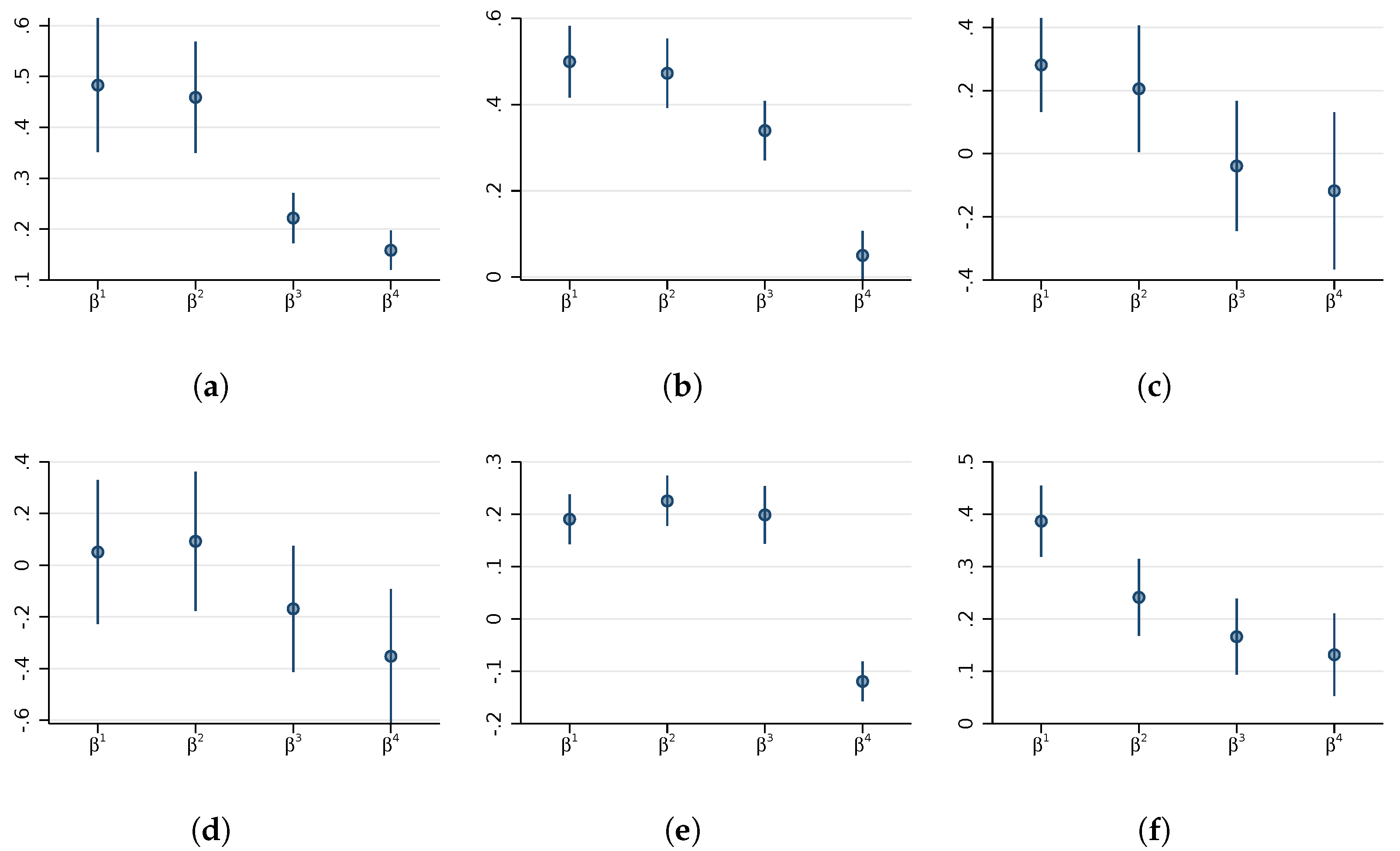
Our parameter of interest,
, is the income elasticity of nighttime lights, a unitless measure indicating the percentage luminosity increase in response to a one percent change in GDP. We estimate this parameter separately for subsamples split according to quartiles of average GDP to obtain four coefficients (
for
). These four groups of different average GDP are a proxy for subnational differences in statistical capacity. Under the conditional mean independence assumptions typically made in the related literature [
2,
3,
26] the resulting estimates will converge to the true coefficient times an attenuation factor. If the true relationship were constant across all subsamples of the data and the variance of the measurement error in GDP were constant, then the estimated elasticities should be very similar in each partition of the data (with some expected sampling variation). More formally,
. If the true relationship is constant but the GDP error variance differs across subsamples, then the estimated coefficients will be attenuated differently, such that
. In this case, it is plausible that the highest GDP category would have the smallest measurement error in GDP, resulting in the least attenuation of the coefficient. However, our analysis does not presume any particular pattern of attenuation.
Appendix A derives these results and provides details on the required assumptions.
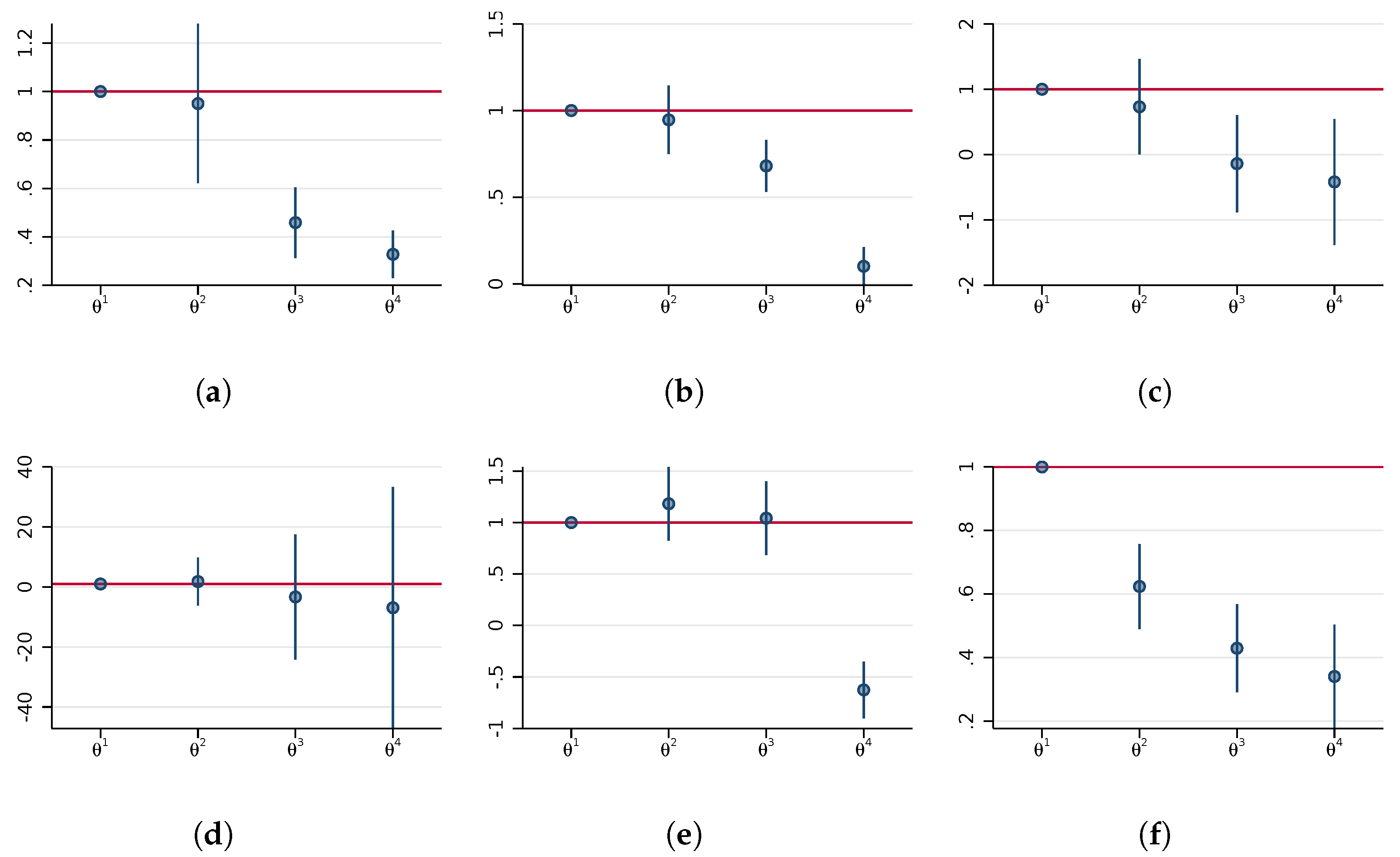
We use this relationship to study whether the differences in elasticities and the implied attenuation factors are plausible. If the true structural elasticity is assumed constant, the ratio of any two point estimates indicates how different measurement errors must be in order explain the variation in the estimated elasticities across the two subsamples. For each country, we estimate and report the ratios comparing the quarter k to the data up to the first quartile. If, for example, the variance of measurement errors in GDP falls with higher incomes, then the sequence of coefficient estimates would be rising and we would interpret a ratio of, say, as ‘the income elasticity of nighttime lights has to be twice as attenuated in the lowest GDP quartile than the highest GDP quartile for the constant elasticity model to be true’. The pattern would be reversed if the variance of measurement errors in GDP increases with income. If we cannot reject the hypothesis that the ratio is different from one, then we conclude that their attenuation factors could have been the same.
Going one step further, we interpret values of statistically different from 1 in countries with high statistical capacity as evidence against the constant elasticity model typically assumed in the applied literature. Of course, it is plausible that the variation in measurement errors of subnational GDP is substantial in developing countries, where there may be more variation in informality across regions, or in the capacity of the statistical apparatus to collect economic data. However, in developed countries with uniformly high statistical capacity, we should not observe significant differences in the signal-to-noise ratio of GDP across regions, and, in fact, expect the estimated s to be close to one. Even if the signal-to-noise ratio in the best measured part of the data were, say, 0.8, then a doubling or halving of this ratio for some regions would imply implausibly large differences in measurement error in high capacity countries. This is why our sample of countries deliberately spans highest quality subnational accounts (the US or Germany) and countries where regional GDP is estimated with less precision (China or Brazil). We use the estimates from developed economies to better understand the relative roles of “structural” nonlinearities and measurement errors in the light-output relationship in developing economies, where nighttime lights are most often used as a proxy for local GDP.
Note that our assumptions measurement errors in GDP and lights also imply that the standard errors of the estimated coefficients are biased. While the sign is indeterminate, it can be shown that the resulting t-statistics are underestimated. The standard errors of the estimated relative attenuation factors are also affected by measurement errors. We leave potential solutions to these issues for future research and note that our estimates of the uncertainties are not free of large sample biases.
Our second approach to studying heterogeneity in the income elasticity models the variation along a third variable:
where
is the logarithm of population density in the first year of the data and all other variables are defined as before. We focus on population density since the light-GDP relationship could vary along this dimension for several reasons. For example, fixed costs of light infrastructure can be large at low population densities, while at high densities, economies of scale and vertical city growth may decrease the responsiveness of lights to changes in GDP.
Given that both light and GDP per area are in logarithms, taking the derivative of Equation (
2) with respect to
results in an elasticity that varies with initial population density. For this specification, we are no longer interested in ratios of these elasticities at different points in the distribution but instead focus on the sign and significance of
. It is important to note that all coefficient estimates in specifications with multiple independent variables, of which at least one is measured with error, are biased in unknown directions. However, if we are willing to assume that population density in the initial year is measured without error and make additional independence and linearity assumptions, then
converges to zero in probability if the constant elasticity model is correct (see
Appendix A for details on these results). Moreover,
will still be attenuated by the same signal-to-noise ratio as in Equation (
1). Hence, we may compare the estimates of
across the long and short regressions and, with some caveats, interpret a significant result on
as further evidence against the constant elasticity model.
Another likely source of structural differences in the nightlight-economic output relationship are differences in industrial composition. For example, if nighttime lights fail to pick up changes in agricultural GDP [
29,
30], then differences in sectoral composition across regions are sufficient to generate variation in the measured light-output relationship. Given that agricultural areas are typically less densely populated than regions with large manufacturing or service hubs, this would also imply some variation of the light-output elasticity with respect to population density. Moreover, it is an open question whether lights primarily respond to value-creation in industry or services and whether the elasticity is constant within each economic sector. Light in densely populated urban areas with a high concentration of services, for example, might not scale linearly in output. To explore this in our data, we run regressions of nightlights on GDP separately for agricultural, industry (including construction), and service sector GDP, with and without interactions with population density. Just as with aggregate output, we cannot simply compare the coefficients for different sectors to gauge whether structural elasticity varies because measurement errors are likely to vary across sectors. Instead, maintaining the same assumption from above, we again ask if the implied relative measurement errors are plausible and check whether the interaction with population density is significant.
Finally, we analyze whether aggregation to geographic units of different shapes and sizes changes the pattern of the resulting estimates. This may occur for two reasons related to our analytical framework. First, aggregating smaller units to larger units could reduce measurement errors in both GDP and lights. For example, county GDP errors due to downscaling state data or workplace versus place of residence mismatches are offset when small regions are grouped together. Similarly, overglow of nightlights into neighboring regions becomes internalized when analyzing larger areas, and the relative importance of topcoding decreases as the size of units increases. A second reason for why aggregation could affect the pattern of elasticities is the grouping of smaller units (with potentially different structural elasticities) into larger, more economically mixed units. Regardless, assessing how geographic scale affects the observed elasticities can help explain the disparate findings documented in the literature, which typically finds large variation in elasticities across countries and across different levels of aggregation within the same country [
18,
19].
Previous research on the Modifiable Areal Unit Problem (MAUP) in urban economics suggests that size and shape of administrative units matters little in comparison to other specification issues but also finds that aggregating to large units can distort the underlying relationship [
31]. No study has systematically examined this problem in the context of nighttime lights and GDP.
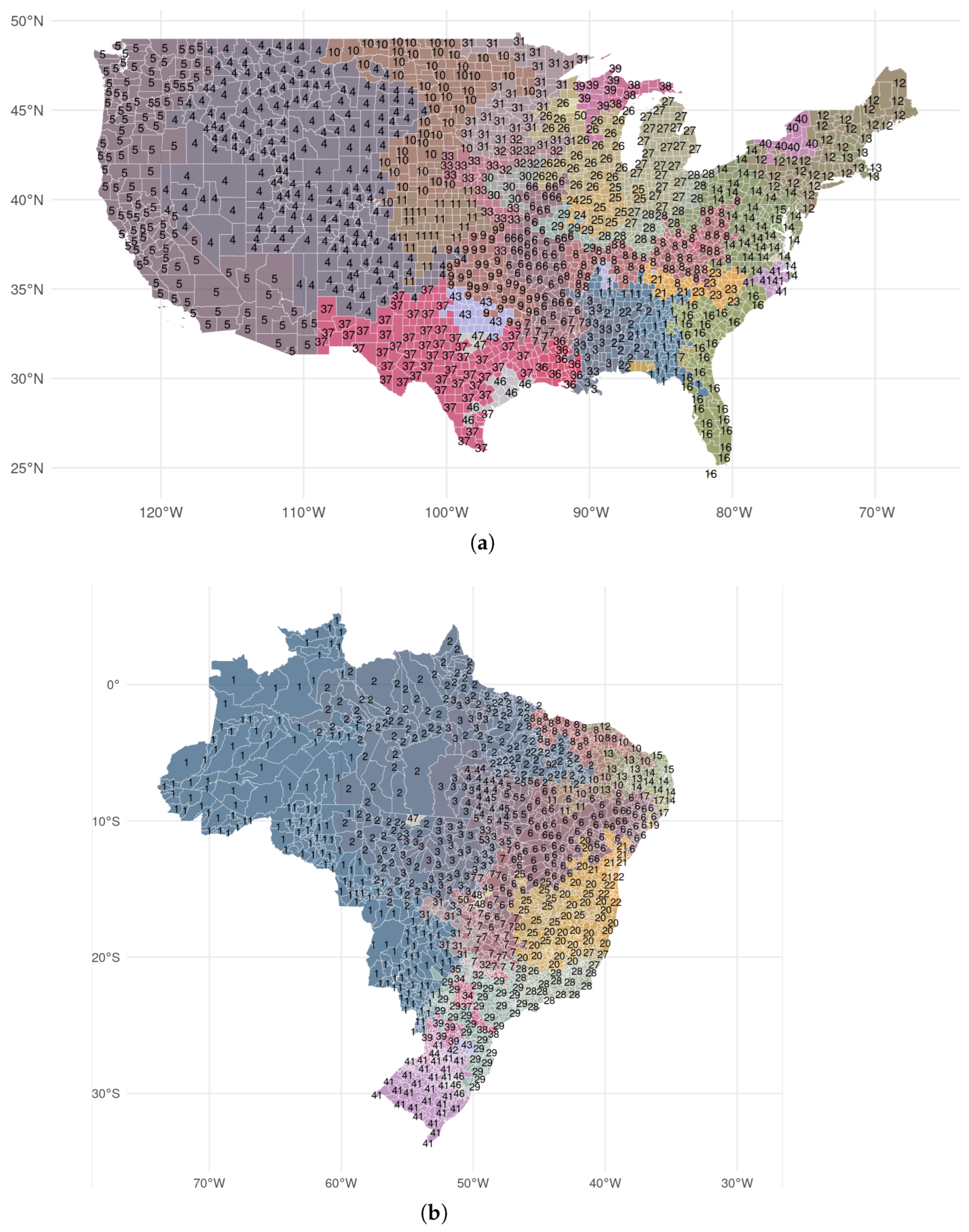
We use methods from the literature on the MAUP [
31,
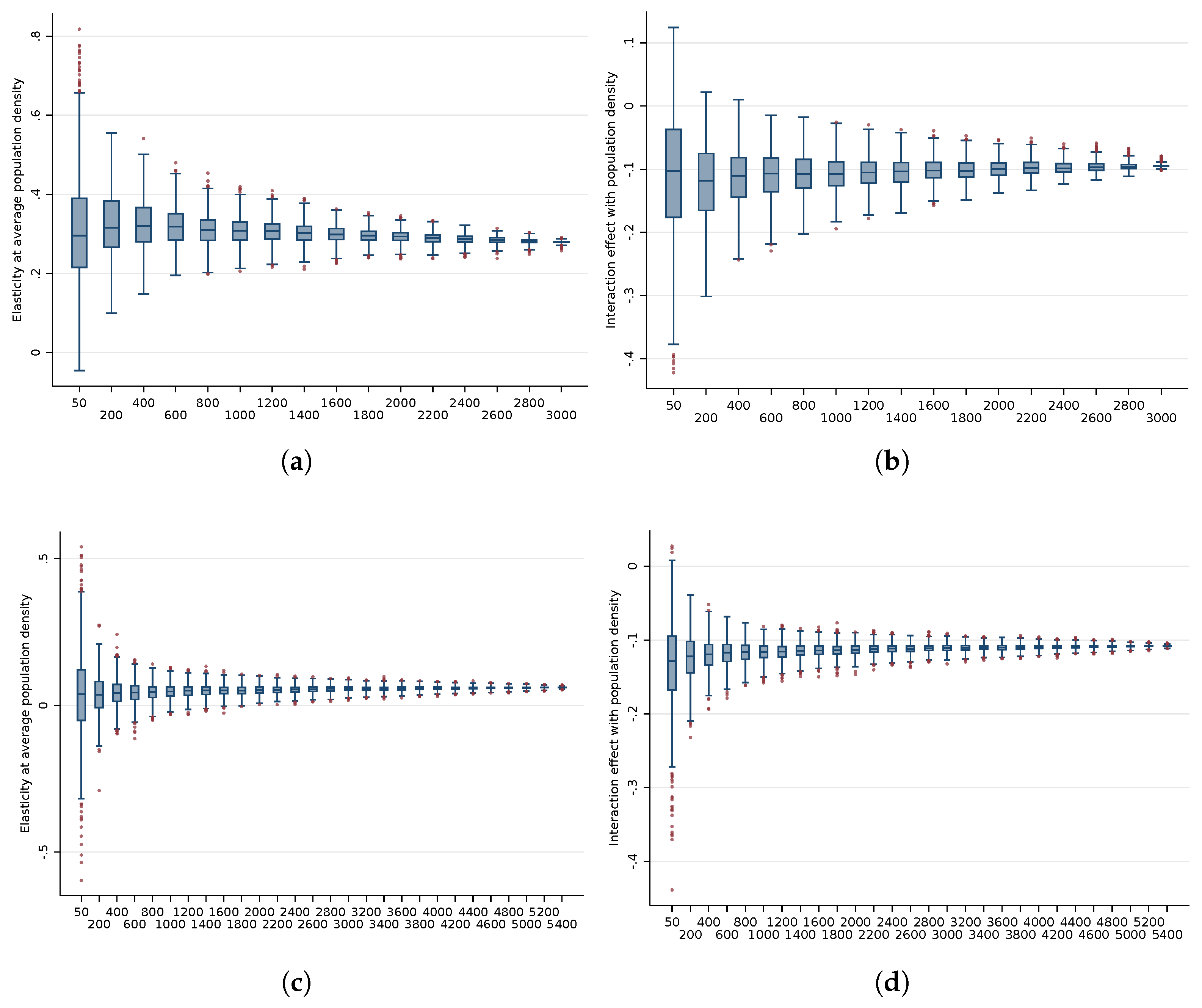
32] to study whether the design of regions creates variation in sectoral composition and population density, which, in turn, generates differences in the structural nightlights-economic output relationship. Specifically, we use disaggregated data on local GDP for the continental United States (3080 counties) and Brazil (5569 municipalities) to create many alternative administrative divisions of varying shapes and sizes. We construct simulated partitions for a given number of administrative units,
k, using the following random-seed-and-grow algorithm [
31]. We start out with the finest level of aggregation into
n units. First, we randomly pick one seed unit. Second, we identify the unit’s closest neighbor before merging these two units so that now there are
units remaining. We repeat these steps until
. The resulting partition is geographically contiguous. We run the algorithm 1000 times for every 200th number of units from
to some country-specific maximum
. We take 50 as a lower bound since this is the number of US states and then simulate the result for
, where
is 3000 for the US and 5400 for Brazil. This results in thousands of alternative divisions of the Unites States and Brazil over which we can aggregate nighttime lights, GDP and population, and estimate the specifications given in Equations (
1) and (
2). A persistence of nonlinearity in simulations with high levels of aggregation (where measurement errors become less severe) would provide additional evidence that the structural elasticity varies.
2.2. Data
We compile data on subnational GDP, sectoral composition, and population from a variety of sources. For each country,
Table 1 lists the smallest geography for which subnational GDP data are available, the number of units, years for which the data are available, the industrial classification used (if available), and the primary source. We deflate current local currency units by the national GDP deflator from the World Development Indicators if the data are not provided in real (constant price) quantities. In the case of the U.S. and European countries, we compute the GDP in each industrial sector by aggregating all NAICS or NACE sectors to a three-sector classification (agriculture, manufacturing and construction, and services). We also obtain high-quality vector geometries representing the geographical units within each country from national statistical offices or other public databases. Data for China is not widely available, which is why we use GDP (in USD) for 299 prefectures from the Economist Intelligence Unit and supplemented this data with information from annual yearbooks and the CEIC’s China Economic Database for the 30 missing prefectures, four municipalities and nine county-level cities.
Measuring economic activity at small geographic scale can be challenging in any country. In addition to the usual data collection and processing errors that arise for national accounts, subnational accounts are particularly prone to non-statistical errors. These include imputations, conceptual differences, index construction, sectoral definitions, and the scope of the exclusions (such as home production, subsistence farming, illegal activity and smuggling) [
33]. Often, subnational estimates of GDP require triangulating with multiple data sources, or downscaling data collected for higher-level administrative regions. This is true even in high statistical capacity countries. In the United States, the Bureau of Economic Analysis relies on the income approach to measure GDP at state and county level, computed as the sum of compensation of employees, taxes on production and imports minus subsidies, and gross operating surplus (capital income). This method has the potential to underestimate capital-intensive industries whose production relies heavily on physical or financial capital [
34]. It measures GDP at people’s place of work, as opposed to place of residence. Interpolation between benchmark years and downscaling from state-level data introduce other sources of measurement error. For example, years when the Economic Census is available (every 5 years) are used as benchmark years, with other years interpolated using sales data from the National Establishment Time Series (NETS) database. In addition, some state-level data on OIC (income payments other than employees and proprietors) are distributed among counties using NETS, the Quarterly Census of Employment and Wages (QCEW), Economic Census data, and industry-specific data from various sources [
35].
Similar methodological challenges exist in the European Union, although analysis on revisions suggest that estimation errors are small (when countries undergo revisions they constitute less than 1% of GDP). However, there are likely to be larger errors in the historical series. Regional GDP is calculated as regional Gross Value Added plus taxes on products minus subsidies. GVA, in turn, is calculated using the production approach (value of output minus intermediate inputs) or the income approach (similar to the U.S.) depending on the member state [
36]. Ongoing work in the European Union is tackling methodological questions for regional GDP such as recording foreign direct investment, non-market services, incorporating global production and integrated global accounts, the digital economy and other price and volume measures for intellectual property products [
37,
38].
Less is known about the quality of subnational accounts in Brazil and China. Brazilian municipal GDP is based on Gross Value Added calculated at state level with the production approach, where state GDP is distributed among municipalities using various methods depending on the good or service [
39]. China officially uses both the production and income methods for national accounts; value-added of agriculture, forestry, animal husbandry and fishery is calculated by the production method, while the current value-added of other industries is calculated using the income method. Regional GDP is measured by local governments using the production approach from major surveys on large industrial firms, large service sector firms, and some construction firms. These data are supplemented by surveys of smaller firms and administrative data from government departments. In addition, they estimate expenditure by household surveys and investment project surveys. Since local Chinese governments are rewarded for meeting growth targets, the Chinese National Bureau of Statistics revises local GDP estimates in computing national GDP [
40,
41].
We obtain nighttime lights within each geography from 1992 until 2013 from the Defense Meteorological Satellite Program (DMSP) Operation Line Scan (OLS) sensors. Specifically, we use annual composites which report yearly average “stable lights” as a 6-bit digital number (DN) from 0 to 63, after observations affected by cloud cover, background noise and other disturbances have been removed. We follow common practice to delete gas flares from the annual composites. Gas flares are disproportionately bright in relation to the change in output they represent and create significant overglow into neighboring pixels. Like Henderson et al. [
3], we also set all pixels that are not on land to zero. For each region-year pair, we calculate the sum of lights and total area of all pixels. Our outcome of interest is the logarithm of lights per area (ln DN/km
).
Table 2 provides the distribution of nightlight density values across subnational regions by country.
Physical detection limits of the DMSP sensors and the difficulty of separating background noise and transient lights from permanent light sources effectively impose a bottom-coding threshold where pixels with DNs of 1–2 and small clusters of pixels with values of less than 4 DN are removed in the stable lights composite. Solutions to this problem range from adding the minimum detection threshold to recorded lights in a region [
5] to using auxiliary data to distinguish background noise from “human lights” [
42]. The problem is most severe in Sub-Saharan Africa, where a lack of consistent electrification implies that mid-sized settlements can be missed. Rural electrification rates are close to 100% in Brazil and China today—the two emerging economies in our data—so we consider this source of error to be less important in our study than others. In fact, very few observations record zero light (see
Table 2).
A potentially serious issue in subnational analyses is that the DMSP data are heavily topcoded. Topcoding primarily occurs in city centers as the sensor gradually reach its saturation limit and affects values well below 63 DN in the yearly averages [
21,
23]. The intensity of topcoding is correlated with our variables of interest, such as average GDP, density, and industrial structure. To deal with this issues, one of our tests uses topcoding corrected data [
23] which applies a Pareto-correction to the stable lights composites (and builds on the radiance-calibrated data available in selected years [
21]).
The DMSP data exhibit overglow or blurring effects for a variety of reasons. The nominal resolution of the data provided by the National Centers for Environmental Information (NCEI) is 30 arc seconds. However, the effective instantaneous field of view (EIFOV) expands from 2.2 km to about 5.4 km at the edge of the scan and the system “smoothes” these data on-board by forming pixel blocks that are 2.7 km by 2.7 km (with different location offsets for each nightly image [
22]). As a result, the same light source will show up in several 30 arc second pixels. On-board processing also magnifies the blur effect for brighter light sources [
22]. Geolocation errors which displace lights by about 3 km exacerbate this problem [
20]. We discuss the biases introduced by overglow
within administrative units when presenting the results and allow for spatial correlation
across units in a robustness check.
A final challenge in using the DMSP data is that the recorded DN cannot be mapped to a physical quantity (radiance). This occurs because the sensors dynamically adjust their low-light detection ability over the lunar cycle but the sensor’s ‘variable gain’ settings are not stored [
21]. Efforts have been made to calibrate using light emitted from islands (such as Sicily) and using active targets for some nights [
43]. However, there are simply no permanently constant light sources on Earth that can unequivocally solve this problem in the historical data, while ad hoc calibration adjustments have the potential to introduce more noise. Another source of variability across years is that the orbit of the DMSP satellites slowly degrades over time, recording lights at a slightly earlier time each day. This feature has recently been used to extend the DMSP data from 2012 to 2019 using pre-dawn data from older satellites that crossed back into a dawn-dusk orbit [
44]. We do not use the extended series as the orbital shift to pre-dawn hours introduces an additional source of measurement error. Following the economics literature [
3], we average the data whenever two years are available and include year fixed effects in all regressions. This accounts for differences in average sensor settings in each year which affect all regions in the same manner. If all pixels were illuminated and topcoding did not exist, then a constant shift in each year would fully account for this problem. However, since differences in gain settings also imply that some pixels cross the detection threshold and others become topcoded before on-board averaging occurs, there is likely to be some residual region-year specific error which cannot be accounted for.
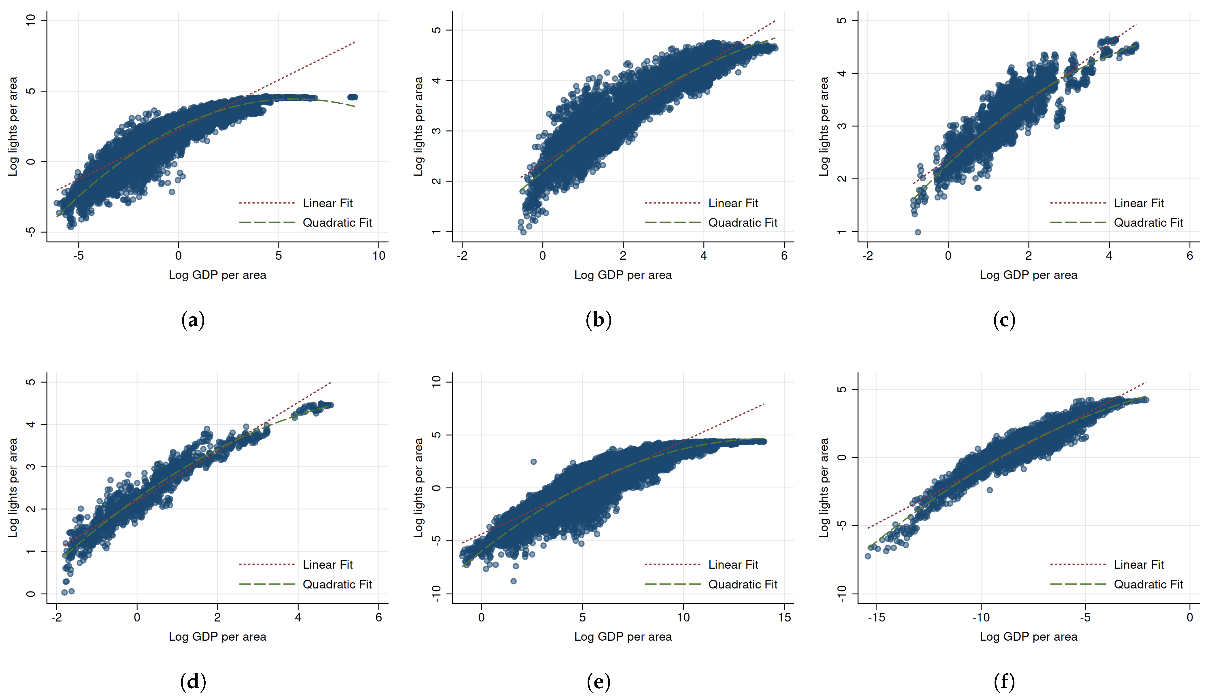
As motivation,
Figure 1 illustrates the raw correlations between light density and economic density. We observe a strong degree of nonlinearity whenever the correlation is based on highly disaggregated data (as in the case of US counties, municipalities in Brazil, and, to a lesser extent, districts in Germany) and less nonlinearity when the data are more aggregated (provinces and prefectures in Italy, Spain and China).


