Article

Deep-Learning-Based Multispectral Image Reconstruction from Single Natural Color RGB Image—Enhancing UAV-Based Phenotyping

1
Graduate School of Agricultural and Life Sciences, The University of Tokyo, Tokyo 113-8657, Japan
2
Department of Electrical Engineering, Indian Institute of Technology, Hyderabad 502284, Telangana, India
3
Agro Climate Research Center, Professor Jayashankar Telangana State Agricultural University, Hyderabad 500030, Telangana, India
4
Department of Genetics and Plant Breeding, Professor Jayashankar Telangana State Agricultural University, Hyderabad 500030, Telangana, India
5
Department of Forest and Soil Sciences, University of Natural Resources and Life Sciences, 1180 Vienna, Austria
*
Author to whom correspondence should be addressed.
Remote Sens. 2022, 14(5), 1272; https://doi.org/10.3390/rs14051272
Submission received: 31 December 2021 / Revised: 23 February 2022 / Accepted: 28 February 2022 / Published: 5 March 2022
(This article belongs to the Special Issue UAVs in Sustainable Agriculture)

Abstract

:
Multispectral images (MSIs) are valuable for precision agriculture due to the extra spectral information acquired compared to natural color RGB (ncRGB) images. In this paper, we thus aim to generate high spatial MSIs through a robust, deep-learning-based reconstruction method using ncRGB images. Using the data from the agronomic research trial for maize and breeding research trial for rice, we first reproduced ncRGB images from MSIs through a rendering model, Model-True to natural color image (Model-TN), which was built using a benchmark hyperspectral image dataset. Subsequently, an MSI reconstruction model, Model-Natural color to Multispectral image (Model-NM), was trained based on prepared ncRGB (ncRGB-Con) images and MSI pairs, ensuring the model can use widely available ncRGB images as input. The integrated loss function of mean relative absolute error (MRAEloss) and spectral information divergence (SIDloss) were most effective during the building of both models, while models using the MRAEloss function were more robust towards variability between growing seasons and species. The reliability of the reconstructed MSIs was demonstrated by high coefficients of determination compared to ground truth values, using the Normalized Difference Vegetation Index (NDVI) as an example. The advantages of using “reconstructed” NDVI over Triangular Greenness Index (TGI), as calculated directly from RGB images, were illustrated by their higher capabilities in differentiating three levels of irrigation treatments on maize plants. This study emphasizes that the performance of MSI reconstruction models could benefit from an optimized loss function and the intermediate step of ncRGB image preparation. The ability of the developed models to reconstruct high-quality MSIs from low-cost ncRGB images will, in particular, promote the application for plant phenotyping in precision agriculture.

1. Introduction

Monitoring plant growth status during the whole growing season is an important objective targeted by multispectral imaging in both breeding and precision agriculture [1,2]. In multispectral images (MSIs), each pixel is composed of reflectance or radiance from multiple discrete wavebands—providing additional spectral information regarding the chemical composition of an object compared to natural color RGB (ncRGB; red, green, blue) images. MSIs can be regarded as a subset of hyperspectral images (HSIs) [3]. With the advancement of sensing technology and data analysis methods, MSIs and HSIs are widely recognized as indispensable tools for continuous and non-destructive monitoring and management in a wide range of fields. However, the broad application of spectral imaging techniques is still restrained due to the higher cost of multi/hyper-spectral sensors and the lower spatial resolution compared to conventional RGB sensors [4,5]. MSI super-resolution through deep learning has become a promising method to recover additional spectral information from RGB images without using more expensive MSI or HSI hardware [6]. MSIs have been shown to be superior in classification tasks compared to corresponding RGB images [7,8]. Optimal waveband selection has been shown to improve the performances of model predictions [9,10]. Furthermore, high spatial resolution hyperspectral images (HR-HSIs) performed better than low spatial resolution ones [11]. Therefore, more readily accessible spectral information beyond the classical RGB bands, preferably at the high spatial resolution, is urgently required to expand the field of application of these techniques.
Recently, ncRGB images have been identified as one possible resource for generating HR-MSIs through deep learning approaches [12,13] because they are widely available worldwide (as captured with consumer-level digital cameras) and generally high in spatial resolution (≥12 million pixels) compared to standard MSIs (~one million pixels, e.g., MicaSense RedEdge™ multispectral band sensor). In contrast, true-color RGB images (tcRGB, i.e., stacked R, G and B bands taken by MSI [14,15,16]), as frequently used for MSI visualization [17,18,19], are generally considered over-saturated (Figure 1) compared to ncRGB images [14,20].
Higher-dimensional hyper-/multispectral information recovery from lower spectral-dimensional ncRGB space is ill-posed in practice [14,21]. Various methods have been proposed to reconstruct HSIs from a single ncRGB image [6,22]. In order to build end-to-end fully supervised models enabling reconstructing MSIs from ncRGB images, the training image pairs (MSIs and ncRGB) have to be established first. The preparation of ncRGB images through conversion directly from MSIs is a more natural approach, as image registration between MSIs and ncRGB images (taken by different cameras) is a complicated task itself and can thus be bypassed [23].
Currently, the generation of ncRGB from MSIs rather than hyperspectral images (HSIs) is hampered because there is a standard approach using well-calibrated spectral response function (SRF) for HSIs while a similar SRF is not available for MSIs [14]. SRF is used to project hyperspectral information to three-dimensional RGB values in natural color through mimicking human perception [24]. Traditional ways of searching for a new SRF were based on hand-crafted priors and strict assumptions [14,25]. In contrast, the potential of deep learning models to directly map MSIs to high-quality ncRGB images through finely tuning non-linear SRFs has not been explored yet [14].
While deep learning is one of the most promising approaches, a bottleneck has been reached to improve deep learning’s performances in hyperspectral information recovery [6]. Specifically, a refined model architecture could only slightly improve the reconstruction accuracy after several years of research. Other components within deep learning should thus be explored regarding their ability to improve model performances—taking advantage of existing architectures. In particular, loss function plays a key role in training deep learning models, measuring the difference between ground truth and predicted values in relative, absolute, squared or angle forms [6]. Two major loss functions, mean squared error (MSEloss) and mean relative absolute error (MRAEloss), have been used widely during the training of models for reconstructing HSIs from single RGB images [6]. However, models trained with both above mentioned loss functions, measuring magnitude differences, still suffer from extensive performance fluctuations in real-world applications [26,27,28]. In contrast, loss functions such as spectral angle mapper (SAMloss) and spectral information divergence (SIDloss), measuring shape similarities between reflectance, can potentially be used to reduce performance variance of models which were trained with magnitude loss functions only [26,29,30].
Taking the different while complimentary properties of these two types of loss functions (i.e., directionless/directional) into consideration, it is tempting to have a composite loss function that can simultaneously measure the differences in magnitude and shape dissimilarities—providing the model an overall “learning direction” during training. Combining two or more algorithms has been shown to feature outstanding performances in material classification, pointing towards the superiority of composite measures of spectra compared to individual ones [31,32,33]. For example, [34] combined both the shape and magnitude of spectra to avoid the limitation of using SAMloss in HSI classification. Unfortunately, models using composite loss functions during training for spectral reconstruction are still rare in precision agriculture.
This study developed and validated a novel method for reconstructing MSIs using ncRGB images of maize and rice plots captured by UAVs. We improved the state-of-the-art deep learning structure HSCNN-R by tuning the number of residual blocks inside the architecture for feature extraction and different loss functions to optimize the model convergence. The enhanced models were used to generate ncRGB images from MSIs and subsequently reconstruct MSIs from ncRGB images. The major contributions can be summarized as follows. First is the derivation of the mapping function converting tcRGB to ncRGB images through training Model-TN based on a benchmark drone HSIs dataset [35]. The mapping function ensured RGB images used for training and future predictions were of a more similar color space, minimizing the performance drop of the RGB color space dependent on MSI reconstruction models. Second is the involvement of combined loss functions in regulating the model convergence. The combined loss functions with complementary properties further improved the model performance. Third, we tested the MSI reconstruction models in real-world experiments. The end-to-end supervised deep learning model (Model-NM) was built based on ncRGB-Con images and MSIs of the maize experiment in 2018. The performances of the Model-NM in recovering multispectral information from RGB images were tested on contrasting testing datasets (i.e., maize data 2019, and rice data 2018) from our experiments. The fidelities of the reconstructed MSIs for phenotyping applications were demonstrated by comparing the calculated Normalized Difference Vegetation Index (NDVI) of reconstructed MSIs from standardized ncRGB images and ground truth MSIs using different growth stages, years and/or crop species. The potential benefits of using NDVI calculated from reconstructed MSIs over Triangular Greenness Index (TGI) based on RGB images for discriminating differently irrigated maize plants were explored to illustrate the application potential of the novel image reconstruction technique in real-world tasks in precision agriculture.
The remainder of this article is organized as follows. The Materials and Methods section describes how different data were collected and used to build different models. The Results section shows the major outcomes from different analyses. The Discussion section mainly discusses the major outcomes of the study and how they were affected by different analyses. The Conclusion section summarizes the study and predicts future research direction on this research topic.

2. Materials and Methods

2.1. tcRGB and ncRGB Image Acquisition from Hyperspectral Images

The true-color RGB (tcRGB) and the corresponding converted, natural color RGB (ncRGB-Con) images, used to build Model-TN (see below), were derived from an HSI benchmark dataset of WHU-Hi-Honghu HSI [35]. The benchmark HSI dataset contains 270 bands from 400 to 1000 nm with a ground sampling distance of about 0.043 m. The tcRGB image was composed of the 33rd, 72nd and 119th bands corresponding to ~475 nm, 561 nm and 668 nm in HSI. The ncRGB images were converted from the HSIs following the procedure described in [14], excluding radiance conversion. In brief, the CIE1934 color response function was used to convert hyperspectral reflectance to a tristimulus vector XYZ and then subjected to linear transformation, non-linear brightness adjustment and finally a threshold of 10−4 was applied to improve the image contrast.

2.2. UAV Image Acquisition of MSI and ncRGB Images from Maize and Rice Fields

Maize (Zea mays L.) plants of the same cultivar were grown on 30 subplots in the field in 2018 (Figure S1a) and 2019 (Figure S1b) in India (N17°19′27.22″, E78°23′55.71″), see [36] for details. Three different irrigation levels were set, i.e., 60% (level 1), 80% (level 2) and 120% (level 3) of cumulative pan evaporation were applied at the subplot level throughout the growing season. Each treatment was replicated three times and randomly distributed as subplots (90) in the field.
In 2018, 160 rice (Oryza sativa L.) cultivars, with two replicates each, were randomly distributed in subplots (320) in the field (Figure S1c) and cultivated following common agronomic practices in India (N17°19′21.55″, E78°24′35.01″).
In both experiments, MSIs and ncRGB images (ncRGB-Cam) were collected simultaneously by different cameras onboard. For MSI acquisition, a MicaSense RedEdge multispectral camera (MicaSense Inc., Seattle, WA, USA) [37] covering 5 wavebands, blue (475 nm, 32 nm bandwidth), green (560 nm, 27 nm bandwidth), red (668 nm, 14 nm bandwidth), near-infrared (840 nm, 57 nm bandwidth), and red edge (717 nm, 12 nm bandwidth) was mounted on an Inspire-1 Pro (DJI, Shenzhen, China) unmanned aerial vehicle (UAV). The onboard RGB camera was Zenmuse X5 (DJI, Shenzhen, China) with a resolution of 16.0 megapixels and ISO range of 100 to 25,600. The flight was set in autopilot mode, flight speed and altitude were 4 km h−1 and 10 m above ground level, respectively. Eighty percent overlap between two consecutive images, containing 1296 × 960 pixels in each band, were realized. Flights were conducted every week around 11 a.m. throughout the growing seasons. Subsequently, specific days of the year (DOY) representing four different growth stages of maize (DOY 303, 313, 323 and 354) and rice (DOY 233, 270, 299 and 328) in 2018, and three different growth stages of maize (DOY 313, 326 and 354) in 2019 were selected for further analysis. Orthomosaics of the entire fields were produced per flight by Agisoft Metashape software [38].

2.3. Model Selection, Training, Validation and Testing

Residual block, which has been used in HSCNN-R [13] previously and shown excellent performance in HSI reconstruction, was used as basic architecture and the number of residual blocks was tuned based on the task complexity in this study. There were 16 residual blocks included in the original architecture which was built to map 3-channel RGB images to 31-channel HSIs for HSI reconstruction. We adapted the output channel number to 3 or 5 based on the number of channels of output images in our study. It has been shown in previous studies that the number of residual blocks was redundant [6,39]. The number of residual blocks was further tuned in this study as well. One residual block was finalized for the ncRGB-Con image production model (Model-True to Model-Natural color image (Model-TN), see below) while three blocks were for MSI reconstruction models (Model-Natural to Multispectral image (Model-NM), see below). The Model-TN (Figure S2) was trained to convert tcRGB images of maize and rice crops to ncRGB ones. Model-NM (Figure S3) was used to recover the multispectral information of the HR-RGB images of maize and rice. HR images are advantageous as the boundaries between different objects can be more clearly set and smaller objects can be more distinguishable, contributing to easier pixel-level semantic segmentation [40]. Contrary to HR features rich in spatial details such as points, lines and local edges, high-level features provide abstract semantic information such as cars, trees and differently irrigated crops [41,42,43]. In order to manage semantic classification tasks well, HR features and high-level features have to be combined [42]. The flowchart of the whole analysis is also supplemented as Figure S4.
Multispectral radiance from the cameras was converted to reflectance based on the known reference panel provided by (MicaSense Inc., Seattle, WA, USA) [37]. RGB images were color corrected with a white reference panel placed inside the field. The RGB images of both benchmark and field experiments were transformed to a range of 0–1 while multispectral images, with reflectance already in the range of 0–1, were used. In order to increase the robustness of both models towards different brightness levels, a random scaling factor (0.1–1.9) was added to each pixel of both input images and output prediction during training [21]. For model training, the batch size was set as 1 and the optimizer Adammax [44] with settings of β1 = 0.9, β2 = 0.999, and eps = 10−8 was selected as default. The weights were initialized through HeNormal initialization [45] in each convolutional layer. The initial learning rate was set at 10−4 and the learning rate decreased by 20% every 5 epochs if the validation loss failed to decrease further. The training of models with composite loss functions is initialized from the weights of trained models with corresponding magnitude loss functions with the same initial learning rate (10−4). All models were trained until no further decrease in validation loss occurred over successive 200 epochs.
The quality of a reconstructed spectrum can be quantified in both magnitude and shape differences when compared to the ground truth one. Three different loss functions were used to either measure magnitude differences, i.e., mean square error (MSEloss; Equation (1); [6,46]) or mean relative absolute error (MRAEloss; Equation (2); [47]), or shape dissimilarities, i.e., spectral information divergence (SIDloss; Equation (3); [26]). Both MSEloss and MRAEloss functions are commonly used while prone to extreme reflectance values [25]. SIDloss has been shown to effectively quantify spectral shape differences regardless of magnitude ones [26]. In addition, two composite loss functions combined measurements of magnitude and shape dissimilarity, i.e., MSE-SIDloss and MRAE-SIDloss. Different weights (W) were assigned to each subcomponent of the composite loss functions: Wmse:Wsid equaled 0.333 and Wmrae:Wsid was 0.0667 throughout the training process to ensure similar contributions to the final loss. The effectiveness of the five different loss functions was compared during model training. Trained Model-TN and Model-NM with the smallest validation losses were selected for further predictions. Three evaluation metrics corresponding to the loss functions, i.e., MRAEev (Equation (4)), RMSEev (Equation (5)), and SIDev (Equation (6)), were used to evaluate models’ performance.
MSE loss = ( 1 n ) i = 1 n ( I gt ( i ) I re ( i ) ) 2
MRAE loss = ( 1 n ) i = 1 n ( | I gt ( i ) I re ( i ) | ) / I gt ( i )
SID loss = ( 1 n ) i = 1 n ( I gt ( i ) | I gt ( i ) | I re ( i ) | I re ( i ) | ) ( log ( I gt ( i ) | I gt ( i ) | ) log ( I re ( i ) | I re ( i ) | ) )
MRAE ev = ( 1 n ) i = 1 n ( | I gt ( i ) I re ( i ) | ) / I gt ( i )
RMSE ev = ( 1 n ) i = 1 n ( I gt ( i ) I re ( i ) ) 2
SID ev = ( 1 n ) i = 1 n ( I gt ( i ) | I gt ( i ) | I re ( i ) | I re ( i ) | ) ( log ( I gt ( i ) | I gt ( i ) | ) log ( I re ( i ) | I re ( i ) | ) )
I gt ( i ) and I re ( i ) represent the ith pixel of the ground truth and reconstructed MSIs, I, respectively.
For Model-TN, original-sized tcRGB and ncRGB-Con images were split into 5 sections: 4 of those were randomly selected for training and the other for validation. The trained model with the best performance was then used for transforming tcRGB images, derived from MSIs of field experiments, to ncRGB-Con images.
During the training of Model-NM, all images of maize collected in 2018 were used for model building, while maize images from 2019 and rice images from 2018 were used for testing—allowing for an independent test of model performance and transferability. Training images were fragmented into 152 patches (size: 512 × 512 pixels) of which 2/3 were used for training and 1/3 for initial validation. These validated models, trained with different loss functions, were subsequently used to reconstruct MSIs of independent testing datasets and further evaluated through three metrics, MRAEev, RMSEev and SIDev at subplot level (Figure S1). The cloud service Google Colaboratory (Colab Pro), 25GB RAM with Python 3 runtime served as the major platform for all model training, validation and testing.

2.4. Ground Truthing of Reconstructed MSIs Using NDVI, and Comparison with RGB-Derived TGI

To illustrate the quality of MSIs reconstructed from standard ncRGB-Con images, the ncRGB-Cam images of maize and rice from the year 2018 were color matched to corresponding ncRGB-Con images rendered from MSIs, before being used to reconstruct high spatial resolution MSIs. Mutual information (MI) is the Kullback divergence between the joint probability density function (PDF) of observed values over local patches of the two images and the product of the marginal PDFs of them [48]. MI was calculated to compare similarities between ncRGB-Con and ncRGB-Cam image either before or after histogram color matching; MI reaches its maximum of one when two images are the same. The quality of the reconstructed MSIs was further assessed through comparisons between calculated NDVI [49] of subplots of MSIs reconstructed from ncRGB-Cam-Con images. Because only plants were of interest when comparing the NDVIs, a threshold of 0.6 was applied to filter out the soil and shadows. The average NDVI of each subplot was calculated and linear regression was used to compare reconstructed and ground truth values.
The NDVIs of reconstructed MSIs from models built on both ncRGB-Cam and tcRGB images were compared so as to highlight the superiority of the intermediate step of natural color conversion from tcRGB to ncRGB-Con.
In order to show the advantages of reconstructed MSIs over indexes derived from ncRGB-Cam, the TGI was calculated based on the color-matched ncRGB-Cam images of maize [50]. The ability of either MSI-derived NDVI or ncRGB-Cam-derived TGIs to reliably separate three levels of irrigation treatments in maize was compared. NDVIs and TGIs of differently irrigated maize plants within each sampling date in 2018 were compared through a permutation test [51] in R [52].

3. Results

3.1. Natural Color Image Rendering
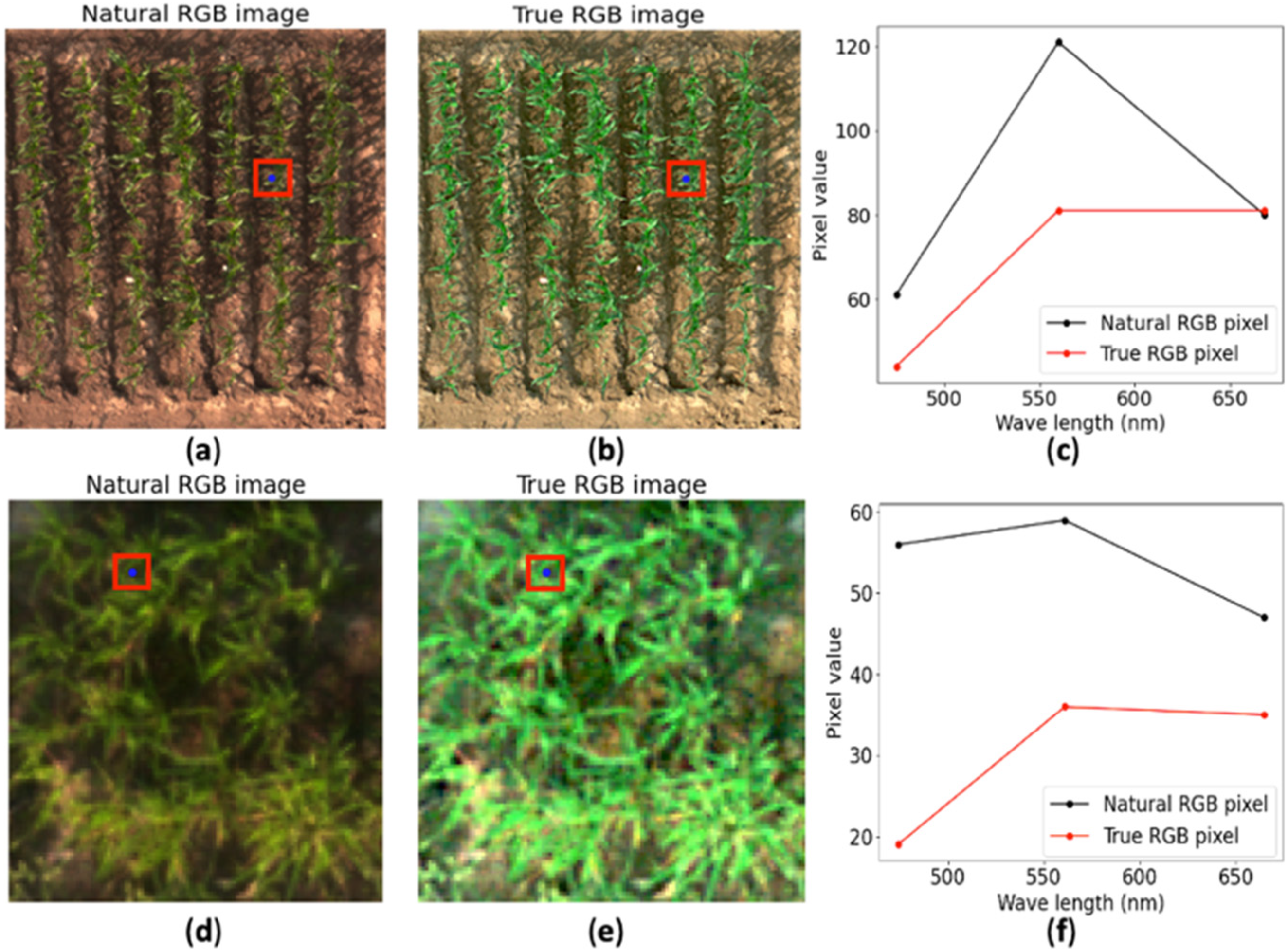
A distinct visual difference was noticed between ncRGB-Con (Figure 1a,d) and tcRGB image (Figure 1b,e) aerial images of maize and rice canopies. The vector of pixel values in corresponding images were distinct in both direction and magnitude (Figure 1c,f). The difference of selected pixels between tcRGB and ncRGB images (see insets in Figure 1) as evaluated by MRAEev, RMSEev and SIDev were 0.233, 0.0934 and 0.0178 for maize, respectively, and 0.932, 0.100 and 0.0701 in rice, respectively.
Figure 1. Converted natural color RGB (ncRGB-Con; (a,d)) and true-color RGB (tcRGB; (b,e)) aerial images, and values of selected pixels (c,f) of maize (ac) and rice (df). The location of pixels is marked by a blue dot at the center of the red box in each RGB image.
Remotesensing 14 01272 g001

3.2. Model Convergence with Different Loss Functions

Both Model-TN and Model-NM, optimized by five different loss functions, had similar performance rankings based on three evaluation metrics (Table 1 and Table 2). Models with MRAE-SIDloss generated minimum total losses of 0.0582 and 0.0571, respectively, compared to models with the other four utilized loss functions. Models with MRAE-SIDloss also predominantly produced the minimum values in each individual evaluation metric, except RMSEev = 0.0127 from Model-TN with MRAEloss with a marginal difference of 0.0001. The second-best loss function was MRAEloss, with a performance close to models regulated by MRAE-SIDloss; the total error differences were marginal as well, i.e., 0.000400 and 0.00310 in Model-TN and Model-NM, respectively. Models with MSE-SIDloss produced errors of 0.258 (Model-NM) and 0.0636 (Model-TN), both being lower than the corresponding models with MSEloss while greater than those of models with SIDloss. Both model types with SIDloss held much higher MRAEev and RMSEev while featuring comparable SIDev compared with models optimized by other loss functions.
Models of Model-TN trained with MSEloss and MSE-SIDloss loss functions had a similar convergence speed, with 3724 and 3729 epochs in 248 and 250 s, respectively (Table 1). Using other loss functions resulted in (considerable) more epochs and time. Models of Model-NM with both MRAEloss and MSEloss loss functions converged at a similar speed of 22,969 and 20,952 s (Table 2), while it took 35,298 s for final convergence when using SIDloss. Noticeably, the two models with composite loss functions consumed much more time compared to those trained with individual loss functions.

3.3. Universality of Models Trained with Different Loss Functions

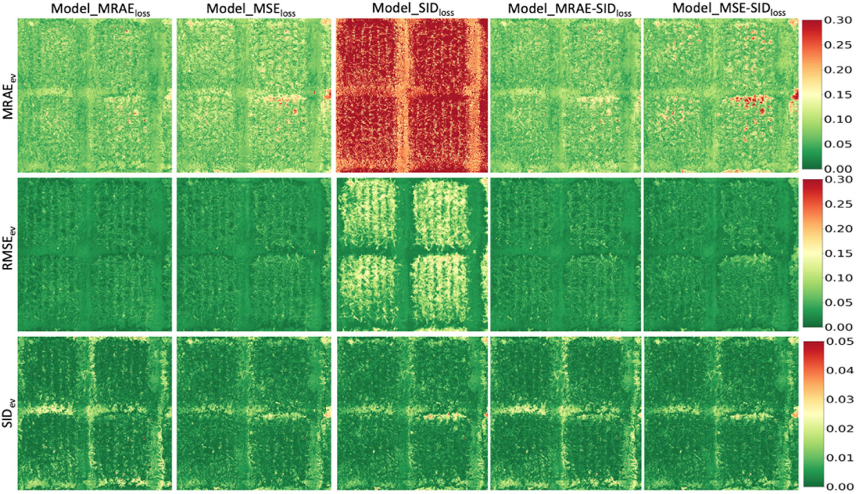
The model performances on the maize testing datasets, evaluated at subplot levels, varied greatly with different loss functions (Figure 2a–c). Models with MRAEloss featured the best performances on testing maize data—indicated by low evaluation values (0.0600, 0.0237 and 0.00348 in MRAEev, RMSEev and SIDev, respectively). In contrast, all models trained with SIDloss had significantly higher magnitude errors (MRAEev = 0.322, RMSEev = 0.0620) compared with other loss functions in maize testing data; nevertheless, they reached a similar level of SIDev compared to the best performing models. The models with the composite loss function MRAE-SIDloss had comparable errors in both evaluations of MRAEev and SIDev as models optimized by MRAEloss.
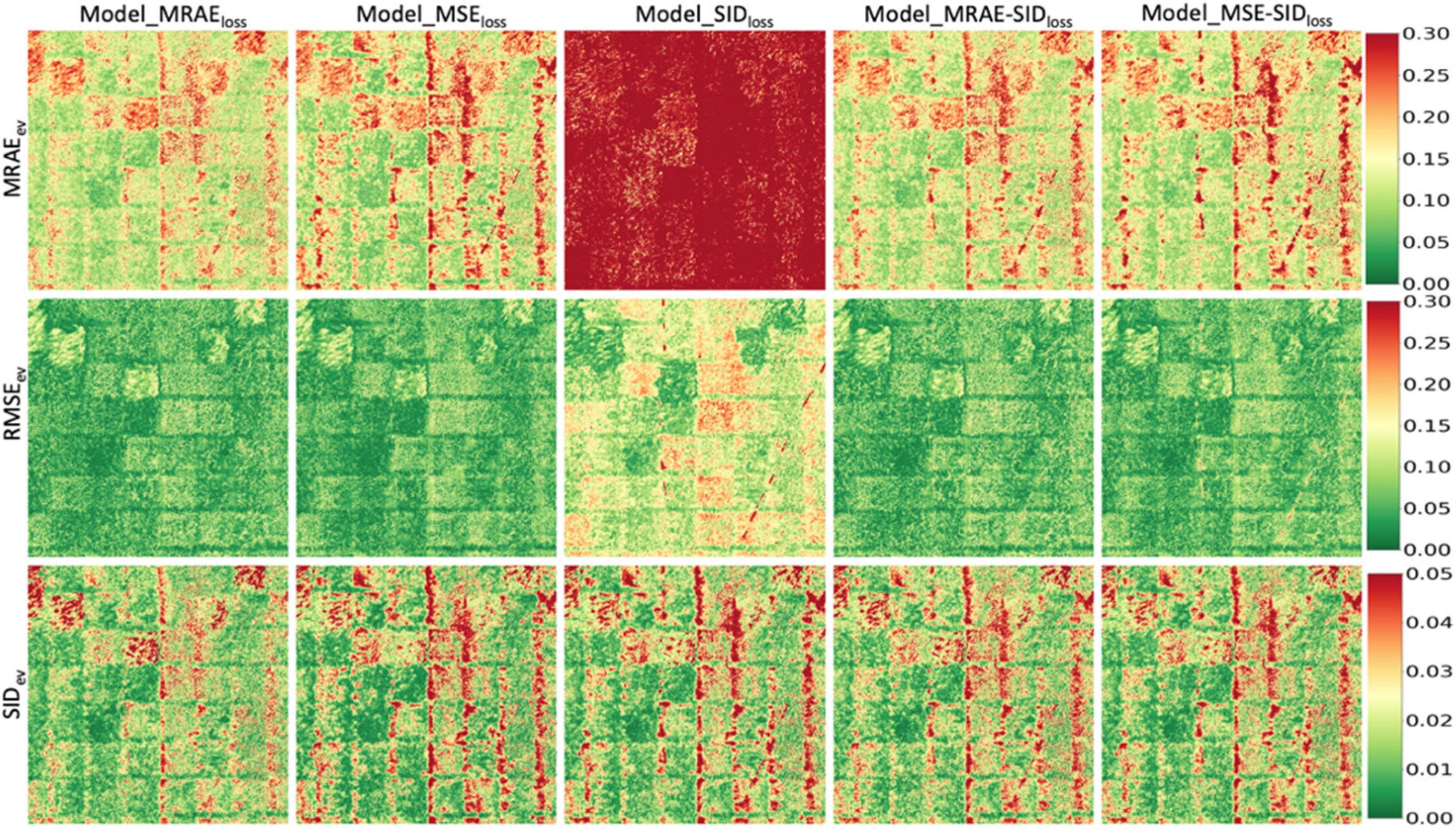
Applied to the rice testing data, the performances of models with different loss functions were similar (Figure 2d–f) compared to the models applied to the maize testing data. Models with MRAEloss performed best in all three evaluation criteria (MRAEev, RMSEev and SIDev of 0.107, 0.046, and 0.012, respectively). SIDloss once more possessed the least generality as suggested by significantly greater errors of MRAEev and RMSEev (0.0363 and 0.0978, respectively) when applied to the rice data. Models trained with MSE-SIDloss had the same level of generality as their corresponding subcomponent, MSEloss, as statistically the same values were produced in all three evaluations. The composite loss function MRAE-SIDloss performed better in MRAEev while worse in RMSEev than the other composite one, MSE-SIDloss. Interestingly, models with all loss functions except MRAEloss reconstructed rice MSIs with statistically the same SIDev.
Visualization of different evaluation metrics on reconstructed MSIs from ncRGB-Con images (Figure S5) of both maize and rice testing data are shown in Figure 3 and Figure 4. More extensive errors of the reconstructed MSIs, indicated by red color, mainly originated from locations with very low reflectance values, such as shadows.

3.4. Effectiveness of MSIs Reconstructed from ncRGB-Cam-Con Images through NDVI and TGI Comparisons

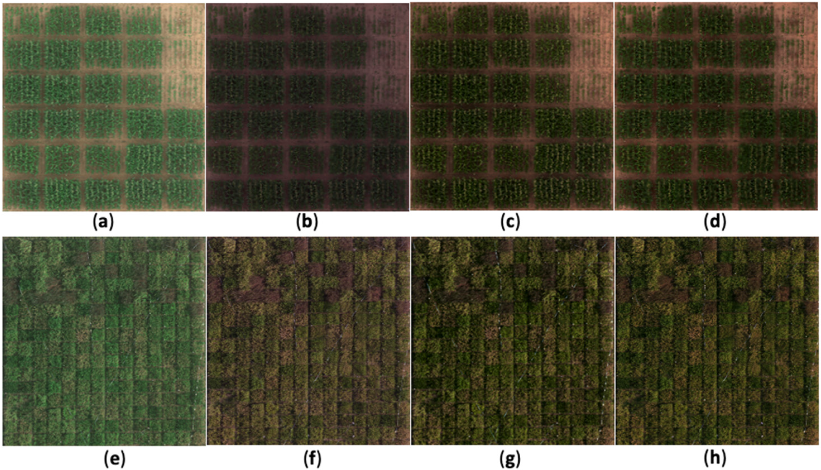
The color differences of tcRGB, ncRGB-Cam, ncRGB-Con and ncRGB-Cam-Con images are exemplified in Figure 5. Even though ncRGB-Con images transformed by the Model-TN looked more natural compared to tcRGB ones, they were still different from directly captured ncRGB-Cam images (Figure 5). The colors of the ncRGB-Cam-Con images (Figure 5c,f) of both maize and rice became more similar to the ncRGB-Con ones (Figure 5b,e)—both by visual impression and MI (Table S1) after color matching. Color matching increased the MI of these ncRGB-Cam testing images of both maize and rice. The minimum increase of MI was 7.55% on maize image on DOY 313 in 2018 while the highest one was on maize on DOY 323 in 2018 with 38.9% after histogram color matching. In rice, the improvement in MI was generally higher than maize images. The smallest increase of MI was 21.3% on DOY 233 in 2018 and the biggest increase was on DOY 270 in 2018 with the value of 135%. The maize image on DOY 354 in 2018 shared the highest MI, 0.65, with the corresponding ncRGB-Con image, while the rice image on DOY 233 in 2018 had the highest agreement with the corresponding converted image, 0.775, after color matching.
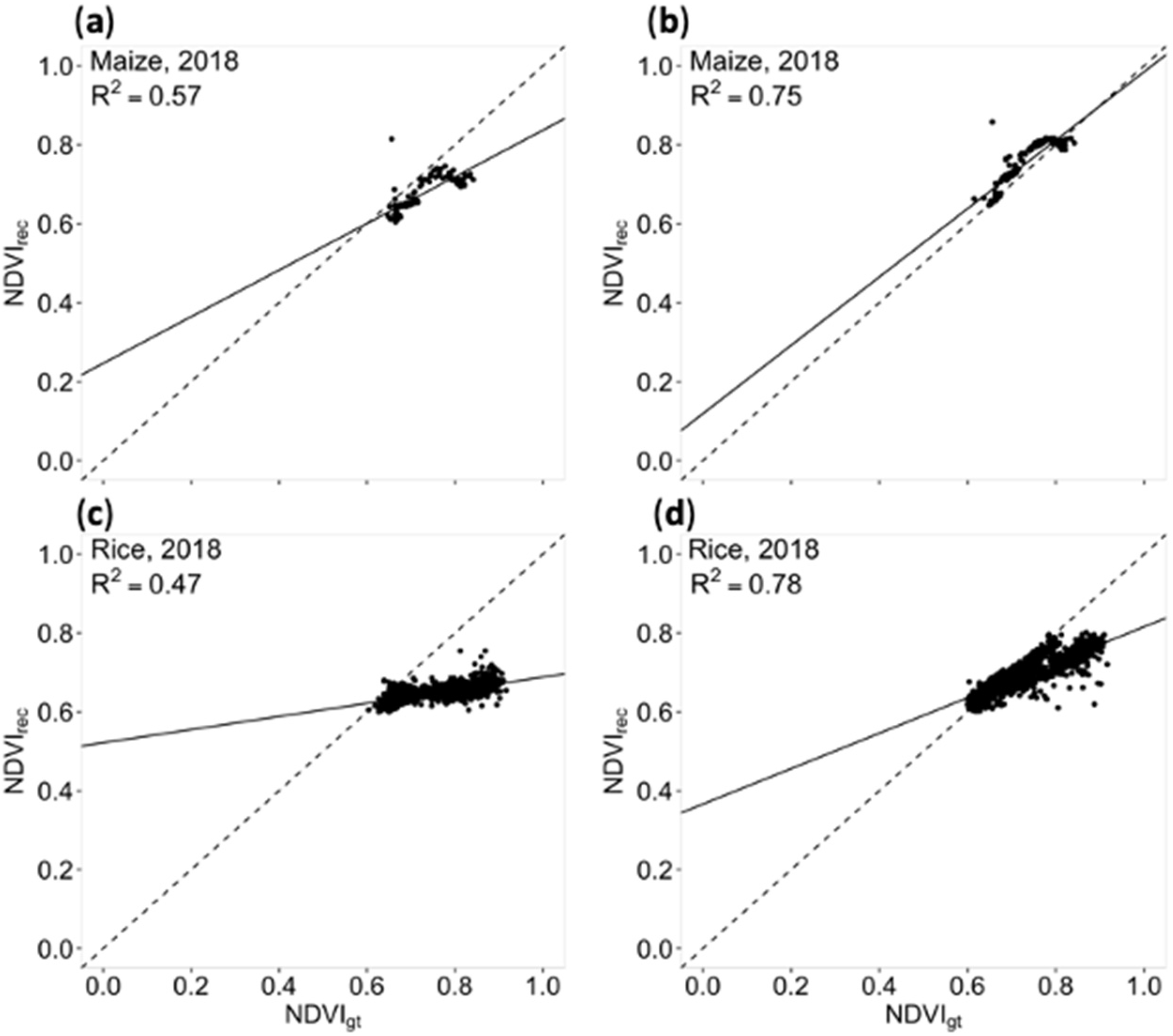
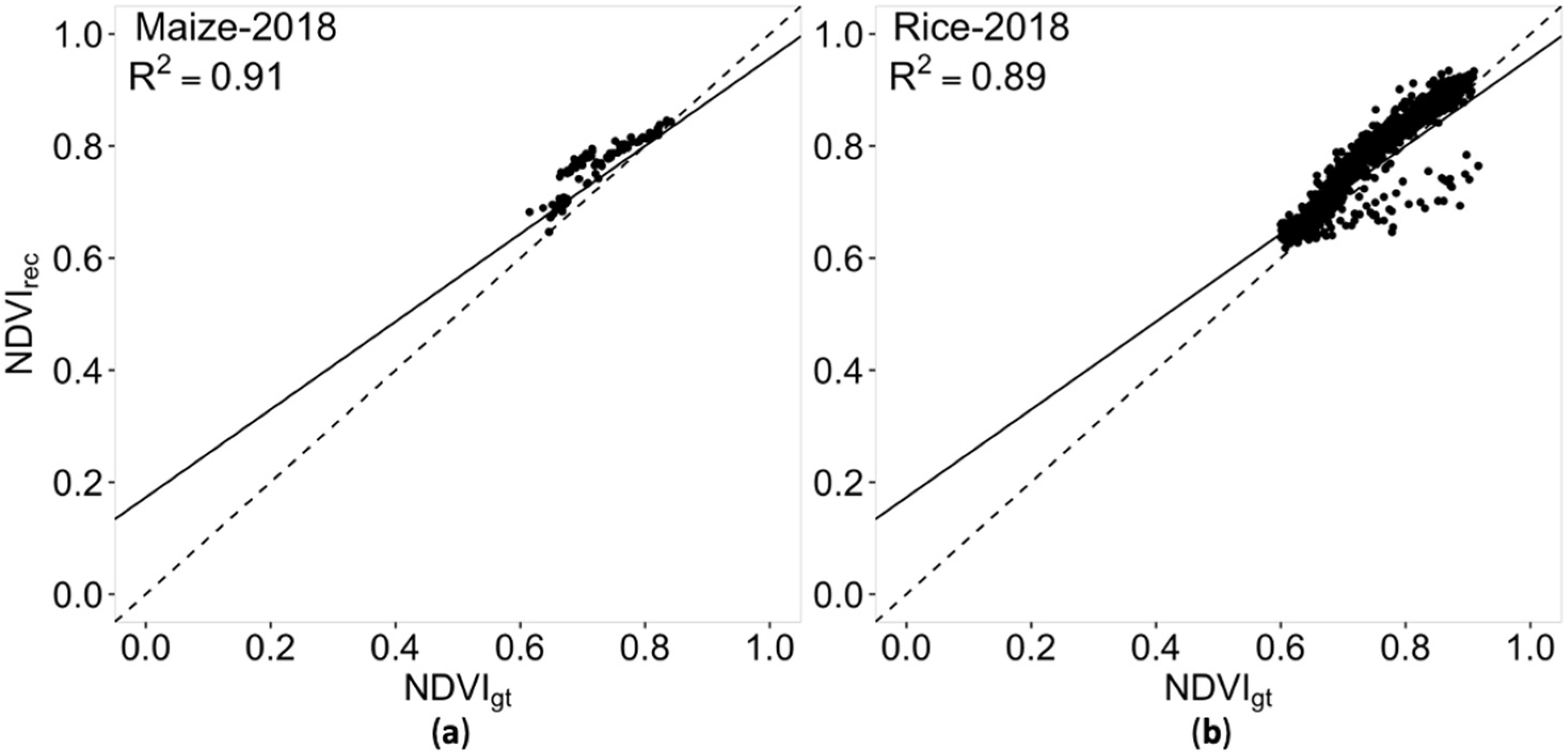
A significant increase in correlation of reconstructed NDVIs with ground truth NDVIS was found when reconstruction models were either built from tcRGB or ncRGB-Con images: 0.57 to 0.75 in maize and 0.47 to 0.78 in rice, respectively (Figure 6). The NDVI calculated from reconstructed MSIs (NDVIrec) values of subplots of ncRGB-Cam-Con images of maize and rice in 2018 reached the highest correlations (R2 = 0.89–0.91) with the NDVI calculated from ground truth MSIs taken directly by a multispectral camera (NDVIgt) (Figure 7).
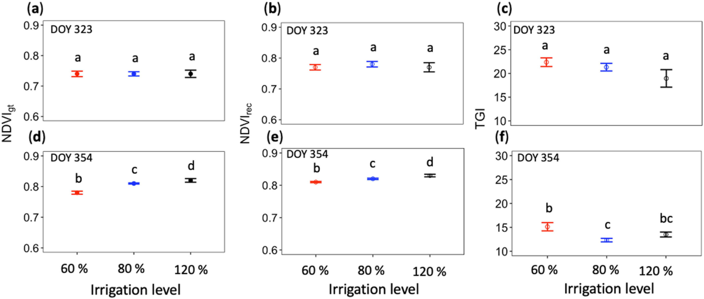
Statistically significant differences of NDVIs of maize leaves among different levels of irrigation were similarly detected by both ground truth MSIs and reconstructed ones from ncRGB-Cam-Con images on DOY 254 in 2018 (Figure 8d,e), while no differences were found between irrigation levels at DOY 303 and 313 (not shown) and DOY 323 (Figure 8a,b).
TGI could not detect the different irrigation levels on maize plants on DOY 354 in 2018, while NDVI was able to do so. Similar to NDVI, no significant differences were found in TGIs of maize plants among different irrigation levels during the first three growth stages, DOY 303 and 313 (not shown) and 323 in 2018 (Figure 8c). Even though TGI values of the least irrigated maize plants (60%) were significantly greater, 19.6, than the other moderately irrigated plants, 16.3, no difference was found between the moderately irrigated maize plants with either of the other two levels of irrigated maize plants on DOY 354 in 2018 (Figure 8f).

4. Discussion

The multispectral information recovery model, Model-NM, has to target ncRGB images for the sake of universality because ncRGB images can be produced easily from low-cost RGB sensors. Models trained on input images of one color type, either true or natural (Figure 1c,f), will perform poorly when reconstructing MSIs from another color space because of the enormous difference in vector magnitude, RMSEev and MRAEev, and directions, SIDev, of pixel values [53]. The performance increase from Model-NM built on tcRGB to Model-NM built on ncRGB-Con images was confirmed by the much more accurate reconstructed NDVIs from ncRGB-Cam images (Figure 6). The recovery of spectral information is thus largely the reconstruction of a higher-dimensional vector from lower-dimension ones, and both the magnitude and direction of the lower-dimensional RGB vector surely affect the reconstruction process [53,54].
The Model-TN was able to produce natural-looking ncRGB images from over-saturated tcRGB images with the help of hyperspectral images, which was an indispensable step to connect MSIs and ncRGB images. Model-TN was trained on benchmark images with various crops, soil and buildings while the maize and rice were not included. Nevertheless, the rendered ncRGB images of maize and rice appeared natural and looked much closer to the color captured by RGB cameras on board based on human perception, indicating a well-polished multispectral response function embedded within the model. Representation of MSIs in ncRGB images is valuable, as the false color tcRGB images can easily lead to misunderstandings during knowledge transferring especially when viewers interpret them based on common sense [55].
The MSI reconstruction model, Model-NM, trained on maize from year 2018, already performed very well on maize of different growth stages from the following year, 2019, and even another crop, rice, at different sampling dates in this study—as indicated by low error rates, green color, of the three applied evaluation metrics on reconstructed MSIs based on models trained with different loss functions, except for ones with SIDloss. The highly accurate reconstructed MSIs at least validated the possibility of MSIs’ recovery from RGB images, which can already offer both researchers and farmers the potential to obtain high-quality MSIs based on standard ncRGB-Cam images.
Fusion of HR-RGB and LR-MSIs is another commonly used approach in spectral image super-resolution. One advantage of fusion strategies over the direct reconstruction ones, e.g., HSCNNR, is that higher quality HR-MSIs can be generated when the super-resolution scale is high (often ≥ 8) [56]. However, the final quality of generated HR-MSIs should not be affected if the super-resolution scale is low, e.g., only 4 in our study. Another advantage of direct reconstruction methods in MSI super-resolution is that the HR-MSIs are reconstructed directly based on the HR-RGB image, taking full advantage of the spatial information of HR-RGB and leading to marginal spatial distortion in the derived HR-MSIs [57]. Additionally, the fusion strategy normally requires a pair of existing low-resolution spectral images and HR-RGB—largely limiting the transferability during practical applications.
Different brightness levels of input images were also covered in the trained models by adding the scaling factor, which changed the brightness from 0.1 to 1.9 times, on input images and reconstructed output as shown in [21], which could be inferred from the excellent performance of the trained models on various testing images in the field. The brightness invariant property is important because it can be easily affected by many factors such as shutter speed, illumination, and aperture size [53]. Most of the spectral reconstruction studies failed to cover this aspect, resulting in big errors when the various exposure of the RGB images were tested [6]. An earlier study using deep learning to reconstruct spectral image brightness invariantly still failed to manage the task on MSI reconstruction due to the missing standard function converting MSIs to ncRGB images [53]. Nonetheless, most images are more or less white balanced through either automatic or manual correction in practice. In precision agriculture, either reference reflectance panels or Downwelling Light Sensor is a must in order to have the comparable reflectance of the crops correctly calculated in time series and environment changing measurements [58]. Even though it is not strictly necessary to train a model to have brightness differences considered, it is still appealing if the model could handle it well. The brightness invariant property of the trained model also guaranteed a much greater potential and robustness towards various real-world situations.
The trained brightness invariant models could still not handle shadow well. Brightness is a matter of light intensity changes, i.e., differences in magnitude, while the spectral shape remains relatively constant [53]. In contrast, shadows affect both the shape and magnitude of the spectrum due to heterogenous illuminations and geometric structure of objects [59]. Shadows are unavoidable for field images and reflectance values were generally much lower, which can be close to 0 in all wavebands, compared to well-illuminated conditions [60], making them prone to have large MRAE errors during spectral reconstruction. Nansen et al. [61] found that one model developed on crops under lighting conditions failed to work on the same crop under shade conditions. The unpredictable properties of spectra due to shadows might be one of the biggest obstacles reducing the generality of the trained models, as no spectra under shadow are alike. Shadow removal, which has been studied extensively in recent years, should thus be one challenge to further improve the model performance [62,63,64].
In brief, loss functions regulate the “direction” towards which the model will learn. Regardless of its high importance, loss function optimization in spectral construction tasks has been much less studied than architectural changes and other hyperparameter tuning in deep learning [39]. Directionless loss functions such as MSEloss and MRAEloss were commonly used in deep learning, in particular, in most scenarios including spectral reconstruction. In contrast, direction sensitive loss functions such as SIDloss and SAMloss were previously mostly used on hyperspectral images for spectral matching during multi/hyper-spectral image exploration [6,65]. Considering the practical applications of spectral imaging, the bias of using MRAEloss in training spectral reconstruction models is much smaller compared to models trained with MSEloss—as the integrity of the whole spectrum is of interest [13,39]. The superiority and consistency of models trained with MRAEloss were also confirmed by Zhao et al. [39]. SIDloss, however, was only able to regulate the shape of reconstructed MSIs, leaving other magnitude-related errors to be enormously high [26]. If aiming to reconstruct MSIs as close to ground truth values as possible and obtaining physically plausible ncRGB images converted from reconstructed MSIs [21], SIDloss will thus not be an option. Nonetheless, due to the fact that most spectral matching assignments are searching spectral signatures for separating different materials or objects, SIDloss is still essential in spectral studies.
The more overall difference a loss function can measure, the better the model can possibly be regulated. In this study, models trained with the composite loss function, MRAE-SIDloss, featuring complementary properties, constantly possessed a better performance compared to models with individual subcomponents. While it was shown earlier that MRAEloss worked more effectively than MSEloss [39], the composite loss function possessed an even better performance compared to MRAEloss alone because of the extra regulation on the shapes of spectra, specifically during model convergence. The below-average performance of models with MSE-SIDloss might be due to the lower capability of the MSEloss component in managing the bias towards outliers or high reflectance values, analog to the limited performance of models trained with MSEloss alone. The contributions of subcomponents were set to equal in this study. However, more efforts in tuning different ratios of them might further improve the model’s final performance but were beyond the scope of this study.
The performances of trained models with different loss functions on new datasets were not consistent with the ones on training sets. Models with composite loss function, MRAE-SIDloss, fell short compared to models with MRAEloss, which is also common in deep learning due to overfitting issues [39]. Deformed spectral reflectance due to shadows also makes the model harder to generalize (see discussion above). Moreover, it has been shown that performances of the spectral reconstruction models were partially dependent on the spatial pattern of the image objects [6]. This may explain why all evaluations ended with lower error values in testing maize plants from another growing season, compared to rice. As MRAE-SIDloss was able to assist models to converge well in all three tasks, further increasing the diversity or augmenting data during training might be a way to further increase model performance on unseen data. Nevertheless, the overfitted model still had outstanding performance, which was better than most of other loss functions tested, on different testing datasets. NDVI is the parameter indicating the chlorophyll content [49], and is frequently used to create biochemical maps of field crops in precision agriculture. The fidelity of reconstructed MSIs can also be partially speculated by whether NDVIs calculated from reconstructed images match with the ground truth values from MSIs, particularly if they can be similarly used to detect plants that were watered differently. The NDVIs showed significant differences among different levels of irrigation at the last growth stage of maize plants. Even though the R2 of sublots’ NDVIs of rice data were not as high as the ones of maize, this was quite reasonable, as the canopy structures between maize and rice were very different which surely affected their spectral reflectance reconstructions [66]. Even though the NDVIs calculated from MSIs which were reconstructed directly from ncRGB-Cam also significantly correlated to the ground truth ones, the relation was further increased, as suggested by higher R2 values, 0.75–0.78 to 0.89–0.91, when ncRGB-Cam images were color adjusted to match ncRGB-Con ones.
The natural color space in which these ncRGB-Cam images locate also affects the final reconstructed MSIs [53]. Histogram color matching was commonly used to correct color differences due to the various light and atmospheric conditions in remote sensing [67,68]. As it is clear that the MIs of all these color-corrected ncRGB-Cam images were subjected to a big increase, even over 100% in rice images, the effectiveness of using histogram color matching in bringing different ncRGB-Cam images to more uniform color space is supported. The color-corrected images share more similar color spaces to corresponding ncRGB-Con images, which is the main reason the reconstructed MSIs had higher accuracy. These indexes generated were more consistent towards ground truth ones, underlining different water treatments. As the spectral response functions of consumer-level cameras vary greatly, resulting in extensive color differences in produced RGB images in practice, these functions are mostly not available for consumers [69]. Transformation of different ncRGB-Cam images of different appearances to the standard format, e.g., ncRGB-Con in this study, should be a more robust method to be explored in order to simplify the reconstruction process and increase the model’s generality at the same time.
The indexes generated from reconstructed MSIs are more consistent with ground truth measurements compared to ones derived from “normal”, broadband RGB images. The most well-known index characterizing the chlorophyll content based on RGB images is TGI [70,71]. TGI also showed the most intimate behavior to NDVI compared to other indexes calculated from RGB images [71]. However, compared with the excellent agreements of NDVIrec, TGIs were not able to show the irrigation differences. It has been shown recently that the TGI calculation depends on the peak wavelength sensitivity, which is affected by the specifications of the Complementary Metal Oxide Semiconductor (CMOS) sensors of the camera used [50]. Even the recalibrated formula calculating TGI, which tried to cover wider CMOS sensitivities, still could not fully cover the variabilities coming from different camera sensors in our study. The reconstructed near-infrared information in MSIs is thus rated indispensable for achieving a higher efficacy in distinguishing maize plants that were differently irrigated.

5. Conclusions

We validated the fidelity of the deep learning model in reconstructing MSIs based on high-resolution ncRGB-Cam images irrespective of brightness levels. We illustrated the benefits of combining complimentary loss functions to supervise the convergence direction of the model on different tasks. The advantage of natural color conversion on tcRGB images in improving the performance of MSI reconstruction models was also highlighted. The model was trained and validated using one crop (maize) imaged in different years and successfully applied on another crop, rice, with a totally different canopy structure. The superiority of the reconstructed NDVIs in separating differently watered maize plants over the frequently used broadband RGB images-derived TGI was endorsed.
The application of reconstructed MSIs in precision agriculture just started and more studies in this area should be conducted, especially targeting image segmentation, object detection and 3D image reconstruction, in which both higher spatial and spectral resolution play more important roles [5,72,73]. During further advancement in this field, some key limitations have to be solved. A more robust mapping function should be developed to connect MSIs to ncRGB-Cam color space rather than a complicated model relying on benchmark HSIs. The establishment of a spectral response function that can translate the reflectance of hyperspectral, multispectral or even RGB images directly to the target ncRGB-Cam image through deep learning is needed. For example, an end-to-end supervised linear neural network with physical constraints applied can be integrated into the reconstruction model. Another issue in multispectral image reconstruction is the ubiquitous existence of shadows. Image pre-processing includes either transforming images to shadow invariant space, or other deep learning methods to remove the shadows before being used for multispectral image reconstruction [74,75]. Once these strategies are incorporated in current reconstruction models, full spectrum reconstruction processes will likely become more precise and thus automatable. Hyperspectral images featuring a higher spectral resolution, thus holding wider application potentials than MSIs, should also be focused on in the future.

Supplementary Materials

The following are available online at https://www.mdpi.com/article/10.3390/rs14051272/s1, Table S1: The Kullback divergence-based mutual information (MI) between on ncRGB-Con image and ncRGB-Cam images of maize and rice on different DOYs in 2018 either without (MIor) or with (MImatched) histogram color matching. Figure S1: Examples of subplots in the fields of maize on DOY 354 in both 2018 (a) and 2019 (b), rice on DOY 328 in 2018 (c). Figure S2: Model-TN for tcRGB to ncRGB image conversion. The architecture of Model-TN composed with only one residual block which is highlighted in dashed box is shown in (a). The whole process of ncRGB image conversion is shown in (b), model training in red box and prediction in blue box. Figure S3. Model-NM for ncRGB image to MSIs conversion. The architecture of Model-NM composed with three residual blocks which are highlighted in dashed box is shown in (a). The whole conversion process from ncRGB image to MSIs is shown in (b). Figure S4: The flowchart of the detailed analysis. Figure S5: The ncRGB-Con images of maize on DOY 354 (a) and rice on DOY 328 in 2018 (b) used for visualization in Figure 3 and Figure 4, respectively.

Author Contributions

J.Z. performed data analysis and drafted the manuscript; A.K., B.N.B., B.M. and P.R. performed the field experiment and collected data; S.N. and W.G. designed the experiment and acquired the funding; all authors contributed substantially to the manuscript preparation and revision. All authors have read and agreed to the published version of the manuscript.

Funding

This study is partially funded by the Japan Science and Technology Agency (JST) and India Department of Science and Technology (DST), SICORP Program JPMJSC16H2, and JST AIP Acceleration Research “Studies of CPS platform to raise big-data-driven AI agriculture”. B.R. was funded by the University of Natural Resources and Life Sciences Vienna.

Data Availability Statement

Not applicable.

Conflicts of Interest

The funders had no role in the design of the study; in the collection, analyses, or interpretation of data; in the writing of the manuscript, or in the decision to publish the results.

References

  1. Zhang, Y.; Han, W.; Niu, X.; Li, G. Maize crop coefficient estimated from UAV-measured multispectral vegetation indices. Sensors 2019, 19, 5250. [Google Scholar] [CrossRef] [PubMed] [Green Version]
  2. DeJonge, K.C.; Mefford, B.S.; Chávez, J.L. Assessing corn water stress using spectral reflectance. Int. J. Remote Sens. 2016, 37, 2294–2312. [Google Scholar] [CrossRef]
  3. Somasegaran, P.; Bohlool, B. Ben Single-strain versus multistrain inoculation: Effect of soil mineral N availability on rhizobial strain effectiveness and competition for nodulation on chick-pea, soybean, and dry bean. Appl. Environ. Microbiol. 1990, 56, 3298–3303. [Google Scholar] [CrossRef] [PubMed] [Green Version]
  4. Cucho-Padin, G.; Loayza, H.; Palacios, S.; Balcazar, M.; Carbajal, M.; Quiroz, R. Development of low-cost remote sensing tools and methods for supporting smallholder agriculture. Appl. Geomat. 2020, 12, 247–263. [Google Scholar] [CrossRef] [Green Version]
  5. Lowe, B.; Kulkarni, A. Multispectral image analysis using random forest. Int. J. Soft Comput. Sci. 2015, 6, 1–14. [Google Scholar] [CrossRef]
  6. Arad, B.; Timofte, R.; Ben-Shahar, O.; Lin, Y.-T.; Finlayson, G.D. Ntire 2020 challenge on spectral reconstruction from an rgb image. In Proceedings of the IEEE/CVF Conference on Computer Vision and Pattern Recognition Workshops, Seattle, WA, USA, 14–19 June 2020; pp. 446–447. [Google Scholar]
  7. Tian, M.; Ban, S.; Yuan, T.; Ji, Y.; Ma, C.; Li, L. Assessing rice lodging using UAV visible and multispectral image. Int. J. Remote Sens. 2021, 42, 8840–8857. [Google Scholar] [CrossRef]
  8. Navarro, P.J.; Miller, L.; Gila-Navarro, A.; Díaz-Galián, M.V.; Aguila, D.J.; Egea-Cortines, M. 3DeepM: An Ad Hoc Architecture Based on Deep Learning Methods for Multispectral Image Classification. Remote Sens. 2021, 13, 729. [Google Scholar] [CrossRef]
  9. Cai, Y.; Huang, H.; Wang, K.; Zhang, C.; Fan, L.; Guo, F. Selecting Optimal Combination of Data Channels for Semantic Segmentation in City Information Modelling (CIM). Remote Sens. 2021, 13, 1367. [Google Scholar] [CrossRef]
  10. Bhuiyan, M.A.E.; Witharana, C.; Liljedahl, A.K.; Jones, B.M.; Daanen, R.; Epstein, H.E.; Kent, K.; Griffin, C.G.; Agnew, A. Understanding the effects of optimal combination of spectral bands on deep learning model predictions: A case study based on permafrost Tundra landform mapping using high resolution multispectral satellite imagery. J. Imaging 2020, 6, 97. [Google Scholar] [CrossRef]
  11. Fu, Y.; Zhang, T.; Zheng, Y.; Zhang, D.; Huang, H. Joint camera spectral response selection and hyperspectral image recovery. IEEE Trans. Pattern Anal. Mach. Intell. 2022, 44, 256–272. [Google Scholar] [CrossRef]
  12. Arad, B.; Ben-Shahar, O. Sparse recovery of hyperspectral signal from natural RGB images. In Proceedings of the 14th European Conference on Computer Vision, Amsterdam, The Netherlands, 11–14 October 2016; pp. 19–34. [Google Scholar]
  13. Shi, Z.; Chen, C.; Xiong, Z.; Liu, D.; Wu, F. HSCNN+: Advanced cnn-based hyperspectral recovery from rgb images. In Proceedings of the IEEE Conference on Computer Vision and Pattern Recognition Workshops (CVPRW), Salt Lake City, UT, USA, 18–22 June 2018; pp. 939–947. [Google Scholar]
  14. Sovdat, B.; Kadunc, M.; Batič, M.; Milčinski, G. Natural color representation of Sentinel-2 data. Remote Sens. Environ. 2019, 225, 392–402. [Google Scholar] [CrossRef]
  15. Su, J.; Liu, C.; Coombes, M.; Hu, X.; Wang, C.; Xu, X.; Li, Q.; Guo, L.; Chen, W.-H. Wheat yellow rust monitoring by learning from multispectral UAV aerial imagery. Comput. Electron. Agric. 2018, 155, 157–166. [Google Scholar] [CrossRef]
  16. Prathap, G.; Afanasyev, I. Deep learning approach for building detection in satellite multispectral imagery. In Proceedings of the 2018 International Conference on Intelligent Systems (IS), Funchal, Portugal, 25–27 September 2018; pp. 461–465. [Google Scholar]
  17. Malla, S.; Tuladhar, A.; Quadri, G.J.; Rosen, P. Multi-Spectral Satellite Image Analysis for Feature Identification and Change Detection VAST Challenge 2017: Honorable Mention for Good Facilitation of Single Image Analysis. In Proceedings of the 2017 IEEE Conference on Visual Analytics Science and Technology (VAST), Phoenix, AZ, USA, 3–6 October 2017; pp. 205–206. [Google Scholar]
  18. Mahdianpari, M.; Salehi, B.; Rezaee, M.; Mohammadimanesh, F.; Zhang, Y. Very deep convolutional neural networks for complex land cover mapping using multispectral remote sensing imagery. Remote Sens. 2018, 10, 1119. [Google Scholar] [CrossRef] [Green Version]
  19. Neagoe, I.; Faur, D.; Vaduva, C.; Datcu, M. Exploratory visual analysis of multispectral EO images based on DNN. In Proceedings of the IGARSS 2018–2018 IEEE International Geoscience and Remote Sensing Symposium, Valencia, Spain, 22–27 July 2018; pp. 2079–2082. [Google Scholar]
  20. Woerd, H.J.; Wernand, M.R. True color classification of natural waters with medium-spectral resolution satellites: SeaWiFS, MODIS, MERIS and OLCI. Sensors 2015, 15, 25663–25680. [Google Scholar] [CrossRef] [PubMed] [Green Version]
  21. Lin, Y.-T.; Finlayson, G.D. Physically Plausible Spectral Reconstruction. Sensors 2020, 20, 6399. [Google Scholar] [CrossRef] [PubMed]
  22. Xiong, Z.; Shi, Z.; Li, H.; Wang, L.; Liu, D.; Wu, F. HSCNN: Cnn-based hyperspectral image recovery from spectrally undersampled projections. In Proceedings of the IEEE International Conference on Computer Vision (ICCV), Venice, Italy, 22–29 October 2017; pp. 518–525. [Google Scholar]
  23. Fu, Y.; Lei, Y.; Wang, T.; Curran, W.J.; Liu, T.; Yang, X. Deep learning in medical image registration: A review. Phys. Med. Biol. 2020, 65, 20TR01. [Google Scholar] [CrossRef] [PubMed] [Green Version]
  24. Fairman, H.S.; Brill, M.H.; Hemmendinger, H. How the CIE 1931 color-matching functions were derived from Wright-Guild data. Color Res. Appl. 1997, 22, 11–23. [Google Scholar] [CrossRef]
  25. Mandanici, E.; Bitelli, G. Preliminary comparison of sentinel-2 and landsat 8 imagery for a combined use. Remote Sens. 2016, 8, 1014. [Google Scholar] [CrossRef] [Green Version]
  26. Chang, C.-I. An information-theoretic approach to spectral variability, similarity, and discrimination for hyperspectral image analysis. IEEE Trans. Inf. Theory 2000, 46, 1927–1932. [Google Scholar] [CrossRef] [Green Version]
  27. Willmott, C.J.; Matsuura, K. Advantages of the mean absolute error (MAE) over the root mean square error (RMSE) in assessing average model performance. Clim. Res. 2005, 30, 79–82. [Google Scholar] [CrossRef]
  28. Franses, P.H. A note on the mean absolute scaled error. Int. J. Forecast. 2016, 32, 20–22. [Google Scholar] [CrossRef] [Green Version]
  29. Yuhas, R.H.; Goetz, A.F.H.; Boardman, J.W. Discrimination among semi-arid landscape endmembers using the spectral angle mapper (SAM) algorithm. In Summaries of the Third Annual JPL Airborne Geosceince Workshop; AVIRIS Workshop: Pasadena, CA, USA, 1992; pp. 147–149. [Google Scholar]
  30. Windrim, L.; Ramakrishnan, R.; Melkumyan, A.; Murphy, R.J.; Chlingaryan, A. Unsupervised feature-learning for hyperspectral data with autoencoders. Remote Sens. 2019, 11, 864. [Google Scholar] [CrossRef] [Green Version]
  31. Du, Y.; Chang, C.-I.; Ren, H.; Chang, C.-C.; Jensen, J.O.; D’Amico, F.M. New hyperspectral discrimination measure for spectral characterization. Opt. Eng. 2004, 43, 1777–1786. [Google Scholar]
  32. Naresh Kumar, M.; Seshasai, M.V.R.; Vara Prasad, K.S.; Kamala, V.; Ramana, K.V.; Dwivedi, R.S.; Roy, P.S. A new hybrid spectral similarity measure for discrimination among Vigna species. Int. J. Remote Sens. 2011, 32, 4041–4053. [Google Scholar] [CrossRef] [Green Version]
  33. Nidamanuri, R.R.; Zbell, B. Normalized Spectral Similarity Score (NS3) as an Efficient Spectral Library Searching Method for Hyperspectral Image Classification. IEEE J. Sel. Top. Appl. Earth Obs. Remote Sens. 2010, 4, 226–240. [Google Scholar] [CrossRef]
  34. Staenz, K.; Schwarz, J.; Vernaccini, L.; Vachon, F.; Nadeau, C. Classification of hyperspectral agricultural data with spectral matching techniques. In Proceedings of the International Symposium on Spectral Sensing Research (ISSSR’99), Las Vegas, NV, USA, 31 October–4 November 1999; Bruzewicz, A.J., Ed.; US Army Corps of Engineers: Hanover, NH, USA, 1999. [Google Scholar]
  35. Zhong, Y.; Hu, X.; Luo, C.; Wang, X.; Zhao, J.; Zhang, L. WHU-Hi: UAV-borne hyperspdectral with high spatial resolution (H2) benchmark datasets and classifier for precise crop identification based on deep convolutional neural network with CRF. Remote Sens. Environ. 2020, 250, 112012. [Google Scholar] [CrossRef]
  36. Kumar, A.; Desai, S.V.; Balasubramanian, V.N.; Rajalakshmi, P.; Guo, W.; Naik, B.B.; Balram, M.; Desai, U.B. Efficient Maize Tassel-Detection Method using UAV based Remote Sensing. Remote Sens. Appl. Soc. Environ. 2021, 23, 100549. [Google Scholar] [CrossRef]
  37. Morales, N.; Kaczmar, N.S.; Santantonio, N.; Gore, M.A.; Mueller, L.A.; Robbins, K.R. ImageBreed: Open-access plant breeding web–database for image-based phenotyping. Plant Phenome J. 2020, 3, e20004. [Google Scholar] [CrossRef]
  38. Lastilla, L.; Belloni, V.; Ravanelli, R.; Crespi, M. DSM Generation from Single and Cross-Sensor Multi-View Satellite Images Using the New Agisoft Metashape: The Case Studies of Trento and Matera (Italy). Remote Sens. 2021, 13, 593. [Google Scholar] [CrossRef]
  39. Zhao, J.; Kechasov, D.; Rewald, B.; Bodner, G.; Verheul, M.; Clarke, N.; Clarke, J.L. Deep Learning in Hyperspectral Image Reconstruction from Single RGB images—A Case Study on Tomato Quality Parameters. Remote Sens. 2020, 12, 3258. [Google Scholar] [CrossRef]
  40. Xu, Y.; Wu, L.; Xie, Z.; Chen, Z. Building extraction in very high resolution remote sensing imagery using deep learning and guided filters. Remote Sens. 2018, 10, 144. [Google Scholar] [CrossRef] [Green Version]
  41. Hua, Y.; Mou, L.; Zhu, X.X. Relation network for multilabel aerial image classification. IEEE Trans. Geosci. Remote Sens. 2020, 58, 4558–4572. [Google Scholar] [CrossRef] [Green Version]
  42. Zhang, Z.; Zhang, X.; Peng, C.; Xue, X.; Sun, J. Exfuse: Enhancing feature fusion for semantic segmentation. In Proceedings of the European conference on Computer Vision, Munich, Germany, 8–14 September 2018; pp. 269–284. [Google Scholar]
  43. Liu, Y.; Cheng, M.-M.; Fan, D.-P.; Zhang, L.; Bian, J.-W.; Tao, D. Semantic edge detection with diverse deep supervision. Int. J. Comput. Vis. 2022, 130, 179–198. [Google Scholar] [CrossRef]
  44. Kingma, D.P.; Ba, J. Adam: A method for stochastic optimization. arXiv 2014, arXiv:1412.6980. [Google Scholar]
  45. He, K.; Zhang, X.; Ren, S.; Sun, J. Delving deep into rectifiers: Surpassing human-level performance on imagenet classification. In Proceedings of the IEEE International Conference on Computer Vision, Santiago, Chile, 11–18 December 2015; pp. 1026–1034. [Google Scholar]
  46. Koundinya, S.; Sharma, H.; Sharma, M.; Upadhyay, A.; Manekar, R.; Mukhopadhyay, R.; Karmakar, A.; Chaudhury, S. 2d-3d cnn based architectures for spectral reconstruction from rgb images. In Proceedings of the IEEE Conference on Computer Vision and Pattern Recognition Workshops, Salt Lake City, UT, USA, 18–22 June 2018; pp. 844–851. [Google Scholar]
  47. Yan, Y.; Zhang, L.; Li, J.; Wei, W.; Zhang, Y. Accurate Spectral Super-Resolution from Single RGB Image Using Multi-scale CNN. In Proceedings of the Chinese Conference on Pattern Recognition and Computer Vision (PRCV), Guangzhou, China, 23–26 November 2018; pp. 206–217. [Google Scholar]
  48. Ceccarelli, M.; di Bisceglie, M.; Galdi, C.; Giangregorio, G.; Ullo, S.L. Image registration using non-linear diffusion. In Proceedings of the IGARSS 2008–2008 IEEE International Geoscience and Remote Sensing Symposium, Boston, MA, USA, 7–11 July 2008; Volume 5, p. V-220. [Google Scholar]
  49. Gitelson, A.A.; Merzlyak, M.N. Remote estimation of chlorophyll content in higher plant leaves. Int. J. Remote Sens. 1997, 18, 2691–2697. [Google Scholar] [CrossRef]
  50. De Ocampo, A.L.P.; Bandala, A.A.; Dadios, E.P. Estimation of Triangular Greenness Index for Unknown PeakWavelength Sensitivity of CMOS-acquired Crop Images. In Proceedings of the 2019 IEEE 11th International Conference on Humanoid, Nanotechnology, Information Technology, Communication and Control, Environment, and Management (HNICEM), Laoag, Philippines, 29 November–1 December 2019; pp. 1–5. [Google Scholar]
  51. Millard, S.P.; Kowarik, A.; Kowarik, M.A. Package ‘EnvStats’. Package for Environmental Statistics. Version 2. 2018, pp. 31–32. Available online: https://cran.r-project.org/web/packages/EnvStats/EnvStats.pdf (accessed on 20 December 2021).
  52. R Core Team R: A Language and Environment for Statistical Computing; R Foundation for Statistical Computing: Vienna, Austria, 2011.
  53. Tarek Stiebel, D.M. Brightness Invariant Deep Spectral Super-Resolution. Sensors 2020, 20, 5789. [Google Scholar] [CrossRef] [PubMed]
  54. Arad, B.; Ben-Shahar, O. Filter selection for hyperspectral estimation. In Proceedings of the IEEE International Conference on Computer Vision, Venice, Italy, 22–29 October 2017; pp. 3153–3161. [Google Scholar]
  55. Scepanovic, S.; Joglekar, S.; Law, S.; Quercia, D. Jane Jacobs in the Sky: Predicting Urban Vitality with Open Satellite Data. Proc. ACM Hum. Comput. Interact. 2021, 5, 1–25. [Google Scholar] [CrossRef]
  56. Wei, W.; Nie, J.; Li, Y.; Zhang, L.; Zhang, Y. Deep Recursive Network for Hyperspectral Image Super-Resolution. IEEE Trans. Comput. Imaging 2020, 6, 1233–1244. [Google Scholar] [CrossRef]
  57. Chen, W.; Zheng, X.; Lu, X. Hyperspectral image super-resolution with self-supervised spectral-spatial residual network. Remote Sens. 2021, 13, 1260. [Google Scholar] [CrossRef]
  58. Mamaghani, B.; Salvaggio, C. Multispectral sensor calibration and characterization for sUAS remote sensing. Sensors 2019, 19, 4453. [Google Scholar] [CrossRef] [Green Version]
  59. Finlayson, G.D.; Hordley, S.D.; Drew, M.S. Removing shadows from images. In Proceedings of the European Conference on Computer Vision, Copenhagen, Denmark, 28–31 May 2002; pp. 823–836. [Google Scholar]
  60. Winkens, C.; Adams, V.; Paulus, D. Automatic shadow detection using hyperspectral data for terrain classification. Electron. Imaging 2019, 2019, 31. [Google Scholar] [CrossRef]
  61. Nansen, C.; Singh, K.; Mian, A.; Allison, B.J.; Simmons, C.W. Using hyperspectral imaging to characterize consistency of coffee brands and their respective roasting classes. J. Food Eng. 2016, 190, 34–39. [Google Scholar] [CrossRef] [Green Version]
  62. Zhang, G.; Cerra, D.; Müller, R. Shadow Detection and Restoration for Hyperspectral Images Based on Nonlinear Spectral Unmixing. Remote Sens. 2020, 12, 3985. [Google Scholar] [CrossRef]
  63. Qu, L.; Tian, J.; He, S.; Tang, Y.; Lau, R.W.H. Deshadownet: A multi-context embedding deep network for shadow removal. In Proceedings of the IEEE Conference on Computer Vision and Pattern Recognition, Honolulu, HI, USA, 21–26 July 2017; pp. 4067–4075. [Google Scholar]
  64. Le, H.; Samaras, D. Shadow removal via shadow image decomposition. In Proceedings of the IEEE/CVF International Conference on Computer Vision, Seoul, Korea, 27–28 October 2019; pp. 8578–8587. [Google Scholar]
  65. Chang, C.-I. Spectral information divergence for hyperspectral image analysis. In Proceedings of the IEEE 1999 International Geoscience and Remote Sensing Symposium (IGARSS 1999), Hamburg, Germany, 28 June–2 July 1999; pp. 509–511. [Google Scholar]
  66. Colwell, J.E. Vegetation canopy reflectance. Remote Sens. Environ. 1974, 3, 175–183. [Google Scholar] [CrossRef]
  67. Haichao, L.; Shengyong, H.; Qi, Z. Fast seamless mosaic algorithm for multiple remote sensing images. Infrared Laser Eng. 2011, 40, 1381–1386. [Google Scholar]
  68. Rau, J.; Chen, N.-Y.; Chen, L.-C. True orthophoto generation of built-up areas using multi-view images. Photogramm. Eng. Remote Sens. 2002, 68, 581–588. [Google Scholar]
  69. Jiang, J.; Liu, D.; Gu, J.; Süsstrunk, S. What is the space of spectral sensitivity functions for digital color cameras? In Proceedings of the 2013 IEEE Workshop on Applications of Computer Vision (WACV), Clearwater Beach, FL, USA, 15–17 January 2013; pp. 168–179. [Google Scholar]
  70. Hunt, E.R.; Daughtry, C.S.T.; Eitel, J.U.H.; Long, D.S. Remote sensing leaf chlorophyll content using a visible band index. Agron. J. 2011, 103, 1090–1099. [Google Scholar] [CrossRef] [Green Version]
  71. Fuentes-Peailillo, F.; Ortega-Farias, S.; Rivera, aM.; Bardeen, M.; Moreno, M. Comparison of vegetation indices acquired from RGB and Multispectral sensors placed on UAV. In Proceedings of the 2018 IEEE International Conference on Automation/XXIII Congress of the Chilean Association of Automatic Control (ICA-ACCA), Concepcion, Chile, 17–19 October 2018; pp. 1–6. [Google Scholar]
  72. Liu, H.; Bruning, B.; Garnett, T.; Berger, B. Hyperspectral imaging and 3D technologies for plant phenotyping: From satellite to close-range sensing. Comput. Electron. Agric. 2020, 175, 105621. [Google Scholar] [CrossRef]
  73. Huang, B.; Zhao, B.; Song, Y. Urban land-use mapping using a deep convolutional neural network with high spatial resolution multispectral remote sensing imagery. Remote Sens. Environ. 2018, 214, 73–86. [Google Scholar] [CrossRef]
  74. He, S.; Peng, B.; Dong, J.; Du, Y. Mask-ShadowNet: Toward Shadow Removal via Masked Adaptive Instance Normalization. IEEE Signal Process. Lett. 2021, 28, 957–961. [Google Scholar] [CrossRef]
  75. Han, H.; Han, C.; Lan, T.; Huang, L.; Hu, C.; Xue, X. Automatic shadow detection for multispectral satellite remote sensing images in invariant color spaces. Appl. Sci. 2020, 10, 6467. [Google Scholar] [CrossRef]
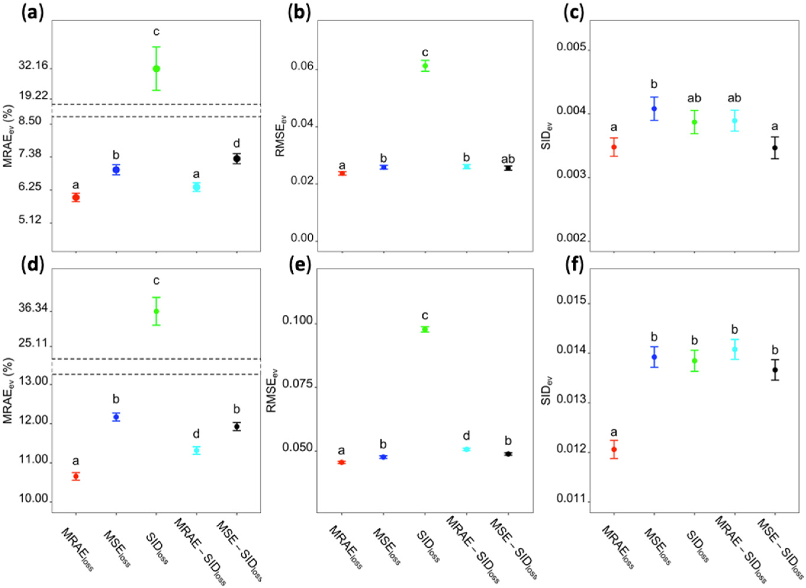
Figure 2. Evaluation of reconstructed MSIs of maize (2019, subplot level, (ac)) and rice (2018, subplot level, (df)) by five loss functions (MRAEloss, MSEloss, SIDloss, MRAE-SIDloss and MSE-SIDloss) using three evaluation metrics (MRAEev, RMSEev and SIDev) (mean ± standard error); see text for details. A total of 90 maize sublots from three sampling dates, and 1680 rice subplots from four sampling dates were analyzed. Different letters in each subpanel indicate a significant difference at the level of 0.05. Note: Differences in Y axis scales; Y axis breaks in subpanels (a,d) for better visualization are indicated by dotted lines.
Remotesensing 14 01272 g002
Figure 3. Visualizations of the evaluations on reconstructed MSIs of maize (2019) based on models optimized with different loss functions. Model_MRAEloss, Model_MSEloss, Model_SIDloss, Model_MRAE-SIDloss and Model_MSE-SIDloss are models trained with five loss functions, correspondingly. MRAEev, RMSEev and SIDev are evaluation metrics on the reconstructed MSIs by corresponding models. Higher errors are indicated by red while lower ones are in green color. See text for details and Supplementary Figure S2a for the ncRGB-Con image.
Remotesensing 14 01272 g003
Figure 4. Visualizations of the evaluations on reconstructed MSIs of rice (2018) based on models optimized with different loss functions. Model_MRAEloss, Model_MSEloss, Model_SIDloss, Model_MRAE-SIDloss and Model_MSE-SIDloss are models trained with five loss functions, correspondingly. MRAEev, RMSEev and SIDev are evaluation metrics on the reconstructed MSIs by corresponding models. Higher errors are indicated by red while lower ones are in green color. See text for details and Supplementary Figure S2b for the ncRGB-Con image.
Remotesensing 14 01272 g004
Figure 5. Example tcRGB images of stacked red, green and blue bands of MSIs (a,e), original ncRGB-Cam images directly taken by onboard RGB camera (b,f), ncRGB-Con images rendered from MSIs by model-TN (c,g), ncRGB-Cam images color matched to ncRGB-Con images (ncRGB-Cam-Con) (d,h) of maize (top row; DOY 354) and rice (bottom row; DOY 328) plots in 2018, respectively.
Remotesensing 14 01272 g005
Figure 6. NDVIs calculated based on reconstructed MSIs (NDVIrec) of ncRGB-Cam images of maize and rice of year 2018 based on models trained on either tcRGB (a,c) or ncRGB-Con (b,d) images of maize 2018 vs. corresponding ground truth MSIs (NDVIgt) taken by the multispectral camera at subplot level. Data of 120 subplots of maize and 1680 subplots of rice were used.
Remotesensing 14 01272 g006
Figure 7. NDVIs calculated based on reconstructed MSIs (NDVIrec) from color-matched ncRGB-Cam (ncRGB-Cam-Con) images of maize (a) and rice (b) of year 2018 vs. corresponding ground truth MSIs (NDVIgt) taken by the multispectral camera at subplot level. Data of 120 subplots of maize and 1680 subplots of rice were used.
Remotesensing 14 01272 g007
Figure 8. NDVI and TGI comparisons between three different irrigation levels of maize on DOY 323 (top row) and DOY 354 (bottom row) in 2018. NDVIgt (a,d) was based on MSIs from the multispectral camera (“ground truth”, gt) while NDVIrec (b,e) and TGI (c,f) were based on MSIs reconstructed from color-matched ncRGB-Cam (ncRGB-Cam-Con) and ncRGB-Cam images, respectively (mean ± standard error). Different letters in each subpanel indicate significance at the level of 0.05.
Remotesensing 14 01272 g008
Table 1. Evaluation of Model-TN (Model-True to Model-Natural color image) with five different loss functions (MRAEloss, MSEloss, SIDloss, MRAE-SIDloss and MSE-SIDloss) by three evaluation metrics (MRAEev, RMSEev and SIDev); see text for details. Model-TN was built to convert tcRGB images from MSIs to ncRGB-Con images of a benchmark dataset. Epochs and time till convergence are given.
Model-TN
Loss FunctionEvaluation Metric
MRAEevRMSEevSIDevTotalEpochsTime (s)
MRAEloss0.04320.01270.002660.058679653510
MSEloss0.05660.01520.004570.07643724248
SIDloss0.46700.08780.003940.55904534512
MRAE-SIDloss0.04280.01280.002610.058286603723
MSE-SIDloss0.04760.01300.003020.06363729250
The minimum values from different evaluation metrics are highlighted in bold.
Table 2. Evaluation of Model-NM (Model-Natural color to Multispectral image) with five different loss functions (MRAEloss, MSEloss, SIDloss, MRAE-SIDloss and MSE-SIDloss) by three evaluation metrics (MRAEev, RMSEev and SIDev); see text for details. Model-NM reconstructed MSIs from ncRGB-Con images of the 2018 maize experiment for model validation. Epochs and time to convergence are given.
Model-NM
Loss FunctionEvaluation Metric
MRAEevRMSEevSIDevTotalEpochsTime (s)
MRAEloss0.03530.01880.006060.0602277722,969
MSEloss0.05340.02090.01190.0862226920,952
SIDloss1.11800.10700.005641.2310299535,298
MRAE-SIDloss0.03440.01730.005410.0571464240,634
MSE-SIDloss0.22500.02660.006140.2580495040,461
The minimum values from different evaluation metrics are highlighted in bold.
Publisher’s Note: MDPI stays neutral with regard to jurisdictional claims in published maps and institutional affiliations.