Article

Winter–Spring Prediction of Snow Avalanche Susceptibility Using Optimisation Multi-Source Heterogeneous Factors in the Western Tianshan Mountains, China

1
College of Resource and Environment Science, Xinjiang University, Urumqi 830046, China
2
Key Laboratory of Oasis Ecology, Ministry of Education, Xinjiang University, Urumqi 830046, China
3
China Institute of Desert Meteorology, CMA, Urumqi 830046, China
4
CAS Research Center for Ecology and Environment of Central Asia, Urumqi 830011, China
5
State Key Laboratory of Desert and Oasis Ecology, Xinjiang Institute of Ecology and Geography, Chinese Academy of Sciences, Urumqi 830011, China
*
Author to whom correspondence should be addressed.
Remote Sens. 2022, 14(6), 1340; https://doi.org/10.3390/rs14061340
Submission received: 11 January 2022 / Revised: 28 February 2022 / Accepted: 4 March 2022 / Published: 10 March 2022
(This article belongs to the Section Remote Sensing in Geology, Geomorphology and Hydrology)

Abstract

:
Data-driven methods are commonly applied in avalanche hazard evaluation. However, few studies have tapped into the relationship between the explanatory variables and avalanche hazard in arid–frigid areas, and the seasonal dynamics of avalanche hazard and its attribution has not been discussed. Therefore, to fill the gap in the hazard assessment of a dry–cold snow avalanche, quantify the dynamic driving process of seasonal nonlinear explanatory variables on avalanche hazard, and improve the reliability of the assessments, this study used Support Vector Machine (SVM), Random Forest (RF) and K-Nearest Neighbour (KNN) algorithms to construct three assessment models; these were used and verified in the western Tianshan Mountains, China. The following results were obtained: The causative factors of avalanches varied based on the season. In winter, terrain and snow depth played a major role, whereas spring was mainly influenced by snow depth and meteorological factors. The dynamic process of avalanche hazard was mainly governed by the seasonality of snow depth and temperature. The seasonal changes in avalanche hazard increased from low to high. The performance of all models was consistent for season and more reliable than the inter-annual evaluations. Among them, the RF model had the best prediction accuracy, with AUC values of 0.88, 0.91 and 0.78 in winter, spring and the control group, respectively. The overall accuracy of the model with multi-source heterogeneous factors was 0.212–0.444 higher than that of exclusive terrain factors. In general, the optimised model could accurately describe the complex nonlinear collaborative relationship between avalanche hazard and its explanatory variables, coupled with a more accurate evaluation. Moreover, free from inter-annual scale, the seasonal avalanche hazard assessment tweaked the model to the best performance.

1. Introduction

Snow avalanches are sudden and destructive natural disasters in mountainous regions of high altitude and low temperature [1,2]. They can fall at a speed of more than 200 km/h, with a pressure of up to 50 t/m2 [3]. Due to the high speed and high pressure, the acting force between avalanche debris and ground objects is extremely destructive; this poses a massive threat to human life and the infrastructure in its path, directly affecting the safety of a mountain’s ecological protective screen, major engineering wiring and social and economic systems [4]. Therefore, hazard modelling and sensitivity mapping in avalanche-prone regions are very important for hazard management, as well as being crucial for targeted disaster adaptation and mitigation.
Avalanche susceptibility modelling is divided into a physical model and a data-driven model [5,6]. Combined with avalanche dynamics and depending on the changes in the characteristics of the snow, such as the gradient changes in temperature, density and moisture content of the snow layer, the physical model evaluates the snow stability and then assesses the avalanche sensitivity [7]. By quantifying the complex effects of weather on the characteristics of snow cover under specific terrain conditions, the Safran–Crocus–Mepra Model Chain infers whether the snow cover in the disaster-pregnant body has the potential of falling [8]. However, the harsh natural environment and poor traffic conditions in alpine regions limit the fine acquisition of background data on meteorology, snow cover, etc. Furthermore, the avalanche-causing mechanism is complex [9], so the constructed physical mechanism model is only applicable to small-scale key areas, which await assessment [10,11]. Applying data mining and machine learning models, numerous studies have used statistical methods to map avalanche susceptibility [12]. Specifically, researchers have focused on the disaster-pregnant environment of avalanches, addressing factors such as meteorology (precipitation, temperature, etc.), topography (elevation, slope, topographic relief, etc.) and human activities, and then assessing the hazard of avalanches based on causality and probability models. In these studies, the meteorological and topographic data selected are easy to obtain, and in a certain range, the statistical algorithm can accurately describe the nonlinear relationship between avalanche activities and the induced conditions. Unlike physical models, none of the parameters are difficult to obtain. Therefore, data-driven models are easier to promote than physical models [13,14]. However, there are practical drawbacks to applying data-driven models, such as the need to subjectively reclassify the selected explanatory variables and assign weights to them [15]. The weighted relationship between avalanche hazard and its nonlinear explanatory variables has not been accurately described. Integrating two or more statistical methods to assess the avalanche hazard has not effectively reduced the one-sidedness and fuzziness in variable selection. Therefore, more self-adaptive models are needed to explore the multidimensional avalanche-related factors, extract variables of avalanche hazards and predict hidden correlations to reduce the uncertainty of data-driven models.
The wide application of machine learning models shows that their modular architecture, such as neural networks, is capable of significantly improving the quality of the results [16]. Deep learning into neural networks would have efficient applications in image processing [17], computer vision [18], meta-materials [19], speech recognition [20] and healthcare [21]. In the field of avalanche research, deep learning algorithms were first used to detect avalanche debris, and applications of some recent sensitivity models [22]—such as the Nearest Neighbouring Method [23], Linear regression (LR) [24], Support Vector Machine (SVM) [25,26], Multivariate Discriminant Analysis (MDA) [27], Random Forest (RF) [28], Naïve Bayes (NB), Classification and Regression Tree (CART), Generalised Additive Model (GAM) [29], Multivariate Adaptive Regression Spline (MARS) and Boosted Regression Trees (BRT) [30,31]—have all obtained promising results (Table 1 lists the advantages and disadvantages of the avalanche hazard assessment methods described above). These studies further demonstrate that the issue of hazard assessment of avalanches has been abstracted into a mathematical model of sample data that can be directly predicted from the intrinsic relationships between the data. Moreover, each algorithm has its own unique characteristics. For example, SVM has strong robustness, high tolerance and high dimensional data processing capability [32]. Therefore, it is more flexible in dealing with nonlinear matters. RF has the advantages of few errors, high accuracy and strong adaptability due to its good tolerance to outliers and noise and due to overfitting. K-Nearest Neighbour (KNN) can process data sets that cannot be explained by linear or curvilinear relations, without making any assumptions about the underlying data; it is also robust to noise and has low restriction towards data types [33]. These studies verified the efficiency of each algorithm in avalanche hazard assessment in different investigated areas. However, to the best of our knowledge, no previous studies have explored the consistency of model efficiency in terms of seasonal variation.
The altitude of the Tianshan Mountains in China’s Xinjiang Uygur Autonomous Region (hereinafter referred to as Xinjiang) markedly decreases from west to east. With the increase in altitude, the spatial and temporal distribution of snow cover in the Tianshan Mountains varies with changes in temperature and solar radiation, and this directly affects the spatial heterogeneity of avalanche hazard. The Tianshan Mountain Range is a complex and magnificent landform. There are many inter-mountain basins and valleys between the mountain chains. Therefore, the avalanche hazard in the Tianshan Mountains is complex and changeable. Moreover, due to the high density of the floating population and the low defence efficiency of disaster prevention strategies, major energy transportation lines and projects along the route are directly exposed to the threat of avalanche. From 1954 to 2018, hundreds of avalanches occurred in this region, causing hundreds of casualties and an annual economic loss of about USD 5 million, according to the local transportation authorities. With the rise in alpine sports and leisure industries and the extension of urbanisation to mountainous areas, the frequency and density of people traveling to alpine areas are increasing, leading to increased avalanche hazards. The exposure of tourism and transportation routes to significant avalanche threats in the Tianshan Mountains has magnified the conflict between avalanche hazards and human interests. Nearly half a century of disaster prevention efforts has resulted in as the construction of snow troughs, snow fences and avalanche-proof corridors at the locations where traffic had once been blocked. However, these results have come either from trial and error or from passive remedies after the occurrence of a great deal of damage, and there are still areas that have long been susceptible to high avalanche hazard but remain undefended. Consequently, the foundation of disaster prevention and mitigation in China’s Tianshan Mountains is slightly weak. Making decisions before a disaster occurs will scientifically reduce the damage and reverse the long-term passivity of humans in avalanche disaster management. Therefore, it is necessary to conduct more comprehensive studies of avalanche hazards. More importantly, most previous studies have focused on marine avalanches in the Alps and Himalayas. The Tianshan Mountains, and its typical continental dry and cold avalanches, are the areas and types of avalanches that have not been sufficiently studied. There are differences in avalanche hazards in different regions and different types of snow cover; therefore, there is an urgent need to expand research to improve the public’s overall understanding of mountain-related natural disasters and the effectiveness of public hazard communication.
Based on the above-mentioned considerations, this study aimed to establish a framework for assessing the avalanche hazard of dry–cold snow in the western Tianshan Mountains of China. The framework sought to map out the triggers exacerbating avalanche hazard and identify their contribution to characterising seasonal avalanche hazard. The goals of the research focused on improving the reliability of avalanche hazard assessments, the foundation of avalanche prevention, and public awareness of snow safety.
The SVM model, RF model and KNN model were used to evaluate the avalanche hazard in winter and spring. The primary objectives were to:
  • Build a database of safety and hazard samples in winter and spring based on the high-precision and large-capacity avalanche inventory;
  • Optimise the evaluation factors with multicollinearity and relief-F and clarify the key elements that affect avalanche hazard in these two seasons;
  • Predict the susceptibility to avalanches in winter and spring using the SVM model, RF model and KNN model, and interpret the distribution and seasonal characteristics;
  • Verify and compare the performance of the optimised multi-source heterogeneous factor models.

2. Study Area

The research area was Taldasha (43°21′–43°35′N, 84°16′–84°40′E), located in the upper reaches of the Ili River basin in the western Tianshan Mountains, China. The valley of the Taldasha region runs from east to west, and the terrain is high in the east and low in the west. The steep mountains on the north and south sides shape the valley topography of the study area into a unique “V” shape. The altitude of the Taldasha region is 2089–4062 m. The main geomorphic units are intermountain basins and valleys developed along zonal tectonic mountains.
Taldasha is a mountain landform with upper intermediate altitude, steep mountain cuttings and acute undulation. It is a disaster easily pregnant body of a slope avalanche or a trench avalanche. Specifically, 49.78% of the slopes have inclinations between 25° and 45°, and 80% of all avalanches occur on these slopes. Taldasha is also located in the HinduKush–Baikal seismic zone of high intensity and frequency, and shallow-focus earthquakes of M ≥ 4 often occur in the region; thus, 16.07% of the avalanches there are induced by an earthquake. As for the climate, Taldasha is located on the east side of the Ili Valley where there is abundant snow fall; it is covered in snow 151 days each year, accounting for 30% of the annual precipitation. The snow is typically dry and cold, with intense thermal gradient metamorphism in the snow layer and thick frosts, leading to the fragile structure of the snow layer, which often induces avalanches. In the dry and cold winter, which lasts for 6 months, most of the snow falls below the altitude of 3000 m with an average thickness of 80 cm. A snow thickness of more than 70 cm is often accompanied by large avalanches. A northeast wind prevails in the region, and wind erosion often triggers avalanches by transporting snow and destabilising the snow layers. The complex landform, active crustal movement, peculiar meteorological conditions and fragile structural layer of the snow accumulation in the Taldasha mountain range lead to the typical and frequent occurrence of avalanches. Hundreds of avalanches occur in Taldasha every year; they are mainly trench avalanches, slope avalanches and slab avalanches. Dry avalanches usually occur from December to early February; then, due to the increase in temperatures, wet avalanches become dominant. The scales of the avalanches can be medium, large or extra-large with a run-out distance range of 98.09–692.42 m. The maximum avalanche area covers 0.21 km2 and is over 4 m deep.
The G217 road in the region (Figure 1) runs through the middle of the Tianshan Mountains and is an important junction connecting the north and south sections of Xinjiang. The road is also a strategic link to the European continent. However, G217 has been exposed to avalanches for years and has to be closed from September to June, resulting in unpredictable potential economic losses each year.

3. Data Collecting and Processing

3.1. Avalanche Inventory Data

From winter of 2018 to winter of 2019, the first snowfall in the study area occurred on 20 November 2018, and by 15 December 2018, it had snowed 23 times. Avalanches occurred successively in the northwest, southeast and southwest valleys of the study area and lasted until 23 March 2019. The avalanches interrupted traffic and logistics, and the local area suffered economic losses. Fortunately, no casualties were reported. To understand the disaster-pregnant environment of avalanches, and to improve local avalanche prevention and control, three avalanche surveys were conducted to obtain complete and reliable information. To overcome the limitations of a manual investigation due to adverse natural conditions and road closures, a space–air–ground-integrated avalanche survey network was established. Based on this network, data on the spatial location, time, type, size, shape, accumulative yield and hazard of avalanches were collected. The specific methods are described in the next section.

3.1.1. Satellite Observation

The SuperView-1 (SV-1) satellite was launched in December 2016 in Taiyuan, Shanxi Province, China. It is China’s first commercial satellite with centimetre-level resolution. Its detailed parameter statistics are listed in Table 2. SV-1 images from January–February 2019 were collected and used to interpret avalanches.
The low reflectivity of avalanche fragments in the near-infrared band [34] and the “tongue-like” shape of avalanche fragments were the key evidence for interpreting avalanches [35]. Image processing before interpretation included radiometric correction, geometric correction and orthorectification. Moreover, the haze and cloud removal workflow in Geomatica was used to reduce the impact of haze on image quality. The definition of the image was improved by stretching (histogram equalisation) and enhancing the image contrast to obtain reliable avalanche boundaries. Finally, to reduce the possible omissions and misjudgments caused by human subjectivity, the image was divided into 20 sub-regions so that they could be visually interpreted, one by one.
In addition to the above image interpretation methods, auxiliary data (surface cover and slope) were also considered to help eliminate confusing image pixels. The image pixels that could not be determined initially were clarified in the subsequent field survey. For example, slopes with tongue-shaped rough texture and fuzzy accumulation turned out to be patches of snow in a particular terrain. To ensure the purity of the avalanche pixels, the mixed pixels in the boundary were artificially removed.
By interpreting avalanche 742 (shown in red in Figure 2) in the SV-1 images of January 2019 (winter), it was found that the minimum and maximum values of the throw range were 0.01 km and 1.30 km, respectively, and the minimum and maximum areas were 3 × 10⁻⁴ km2 and 9.9 × 10⁻² km2, respectively. Avalanches were mainly distributed in the north-western and southern parts of the study area, and they were relatively scattered in space. By interpreting avalanche 2102 (show in green in Figure 2) in February 2019 (spring), it was found that the minimum throw range was 0.125 km, the longest was 1.875 km and the minimum and maximum of the areas were 7.8 × 10⁻³ km2 and 1.31 km2, respectively. In spring, avalanches were abundant in the southern part of the study area, with few in the northern part. On the whole, they were densely distributed in space, and only the avalanche along the east–west direction of G217 was sporadic. The accuracy of the interpretation results was evaluated using the avalanche inventory determined by field investigation. The following results were obtained: user’s accuracywinter = 0.91 and user’s accuracyspring = 0.94. This fulfilled the requirement for establishing a reliable avalanche database on a regional scale.
In a sense, the purity of safe samples (non-avalanche samples) and hazard samples (avalanche samples) determined the model accuracy. Although the hazard samples selected in the SV-1 images were accurate, extra caution was needed. Therefore, in the actual sample selection process, avalanche samples with a small scale, incomplete path and controversial interpretation were excluded.
Ultimately, 458 hazard samples in winter (show in red in Figure 3) and 277 hazard samples in spring (show in dark blue in Figure 3) were included; the number of pixels was 1.374 × 10⁷ and 5.874 × 10⁶, respectively. At the same time, the areas where avalanches were not observed still had the potential for avalanches to occur. Therefore, to reduce the uncertainty of the safe samples, they were selected in areas with flat land, a depression with a slope less than or equal to 10°, and snow-covered and dense Picea schrenkiana trees. Using this method, 290 safe samples in winter (show in purple in Figure 3) were selected, with a sample size of 1.374 × 107 pixels; 194 safe samples in spring (show in green in Figure 3) were selected, with a sample size of 5.874 × 106 pixels. It is worth noting that, to ensure that the dimension of the samples was the same, the number of similar samples was different in term of seasons, but the number of rasters, namely the sample capacity, was the same.
If the samples overlapped in different seasons, the seasonal and spatial variation of avalanche hazard could not be accurately interpreted. Therefore, to avoid overlapping of similar samples in different seasons, the hazard samples in winter were mainly from new locations. Spring avalanches and repeated avalanches on existing paths were excluded from the hazard samples in winter. The overlapping samples were further checked and removed by adding layers and setting the opacity of the top layer (30%).
To avoid the over-fitting phenomenon in the process of machine learning and to maintain the difference in sample composition between the training set and the testing set, and given the generalisation performance of the model, a ratio of 70% to 30% was considered to randomly distribute the training and testing phases.

3.1.2. Avalanche Inventory Obtained by UAV Photography

In this study, DJI Matrice 200 was used for avalanche investigation in Taldasha. The camera used in DJI Matrice 200 was Zenmuse X4S with 24 mm focal length.
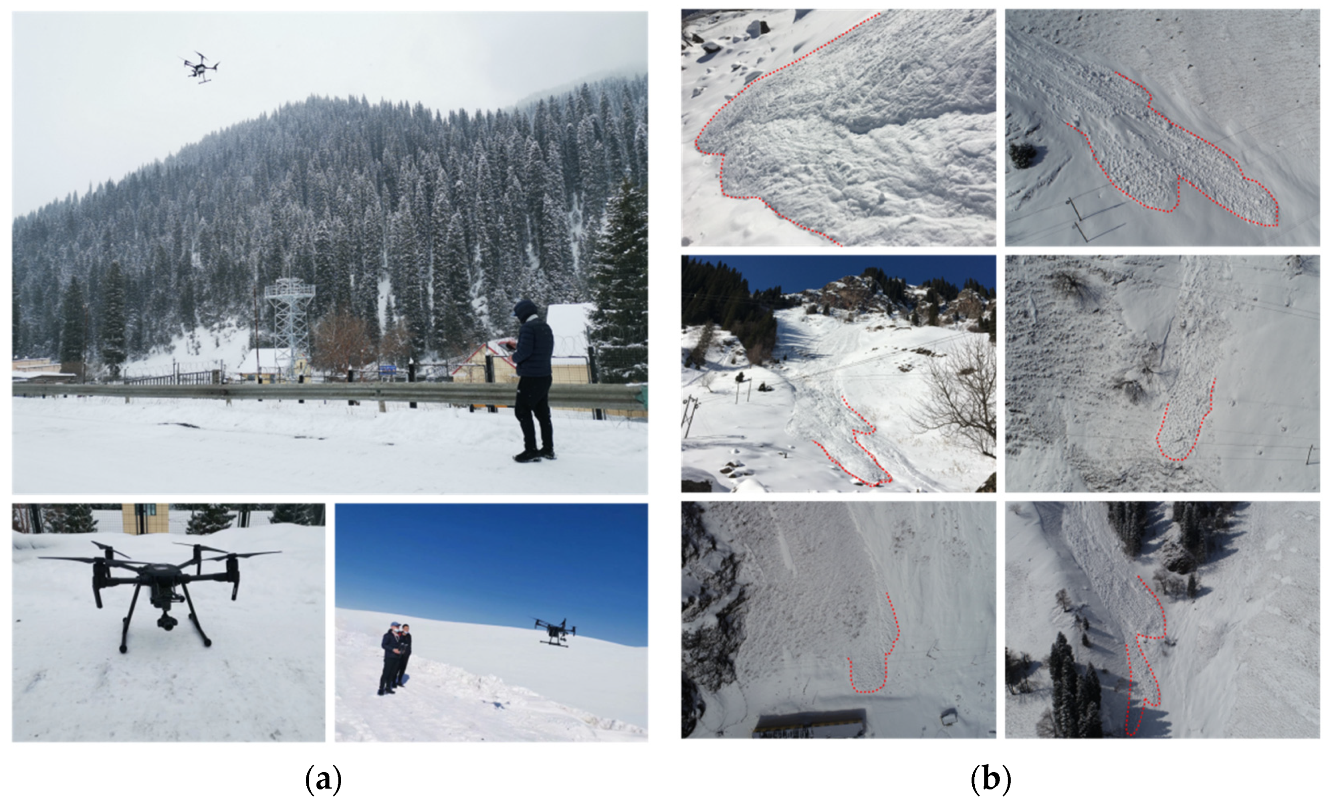
To ensure the quality of images and the safety of UAV (Unmanned Aerial Vehicle), the flight survey was carried out under clear sky conditions with an altitude of 2600–3800 m, a light intensity of greater than 15 lux, a temperature of no lower than −20 °C and wind speed of less than 12 m/s. The operation site is shown in Figure 4a. In this case, three flight routes were designed along the road, and each route was completed in two phases, with a single flight time of about 20 min. For individual avalanche paths disturbed by mist, water vapor or shadows, multiple flights with different altitudes and orientations were used until a satisfactory image was obtained. More than 500 images were captured during the entire process. Orthophoto images of the flight area were created with the help of PhotoScan software.
The avalanche images obtained by UAV are very detailed and accurate. The results of image analysis show that the main avalanche types are groove avalanches, slope avalanches and groove–slope avalanches. They can be small, medium or large. The avalanche debris is roughly tongue-shaped (Figure 4b), which is very important for avalanche interpretation.

3.1.3. Avalanche Inventory from Field Investigation

Artificial avalanche research was carried out along the road in Taldasha, as shown in Figure 5. To make the survey samples more universal and representative, differences in altitude, underlying surface and topography were determined during the field surveys. The physical characteristics of the snow were measured in strict accordance with the guidelines of the IACS (International Association of Cryospheric Sciences), including the depth and particle size of the snow, as well as the temperature, humidity and density of the snow layer.
Based on research and the analysis of the field investigations, it was found that the main factors affecting avalanche induction are terrain, snow depth, temperature, wind speed and crustal dynamics. Among them, 53.66% of avalanches were induced by snowfall and 29.27% by an increase in temperature. Human activity has little to do with avalanche induction. In Taldasha, transport lines, infrastructure, woodland, grassland and bare land are the main victims of avalanches. The local response to avalanches mainly consists of implementing engineering measures, such as metal roof snow fences, protective walls, snow-proof corridors and snow gutters, followed by manual snow removal operations. On the whole, avalanche disaster prevention efforts are weak.
Based on the “air-space-ground” integrated avalanche investigation network, the disaster-pregnant environment for each type of avalanche in Taldasha is basically made clear, and a complete and reliable regional avalanche inventory is mastered. This not only provides a verification basis for this study, but also builds a rich sample database.

3.2. Causative Factors

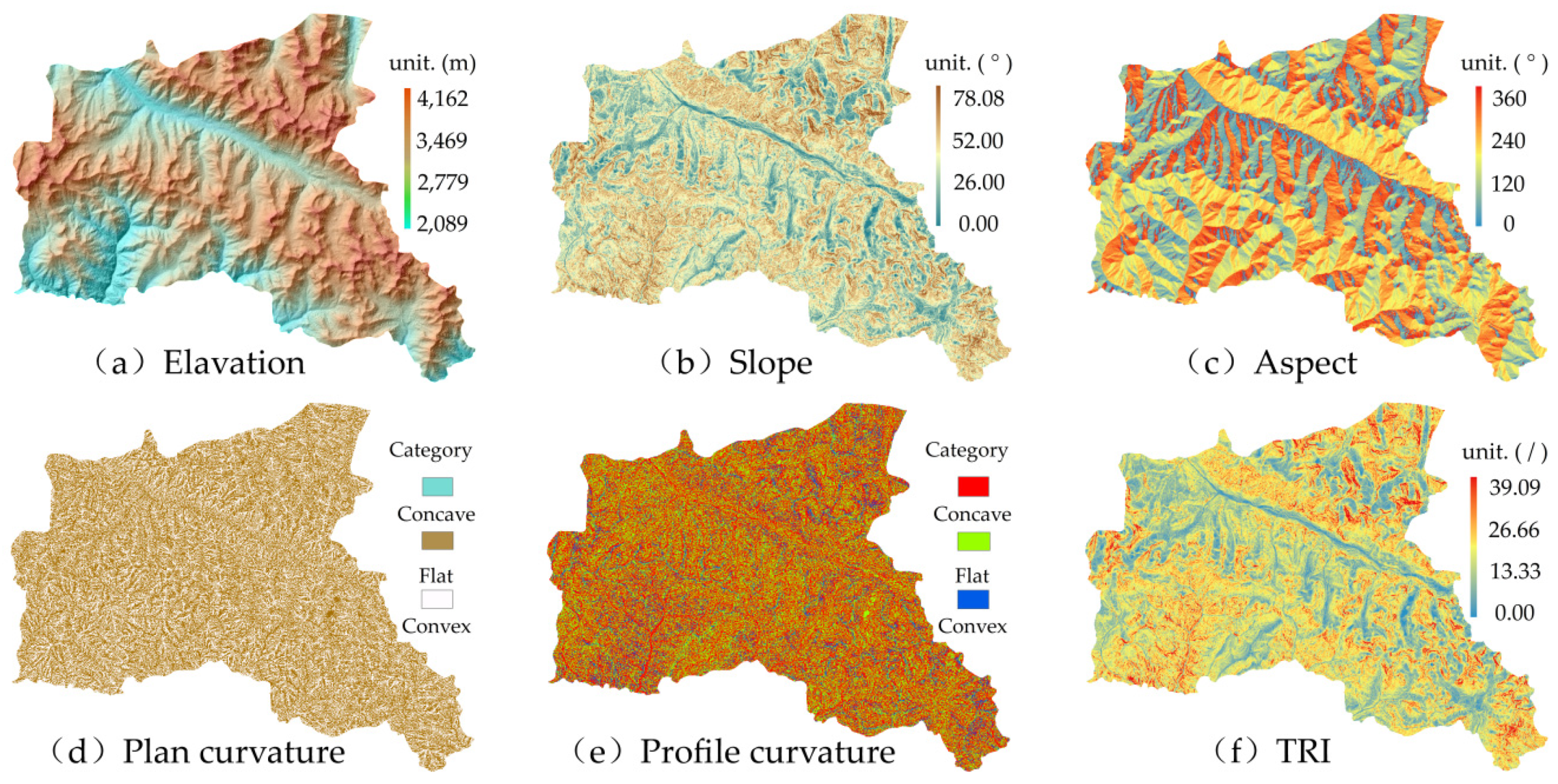
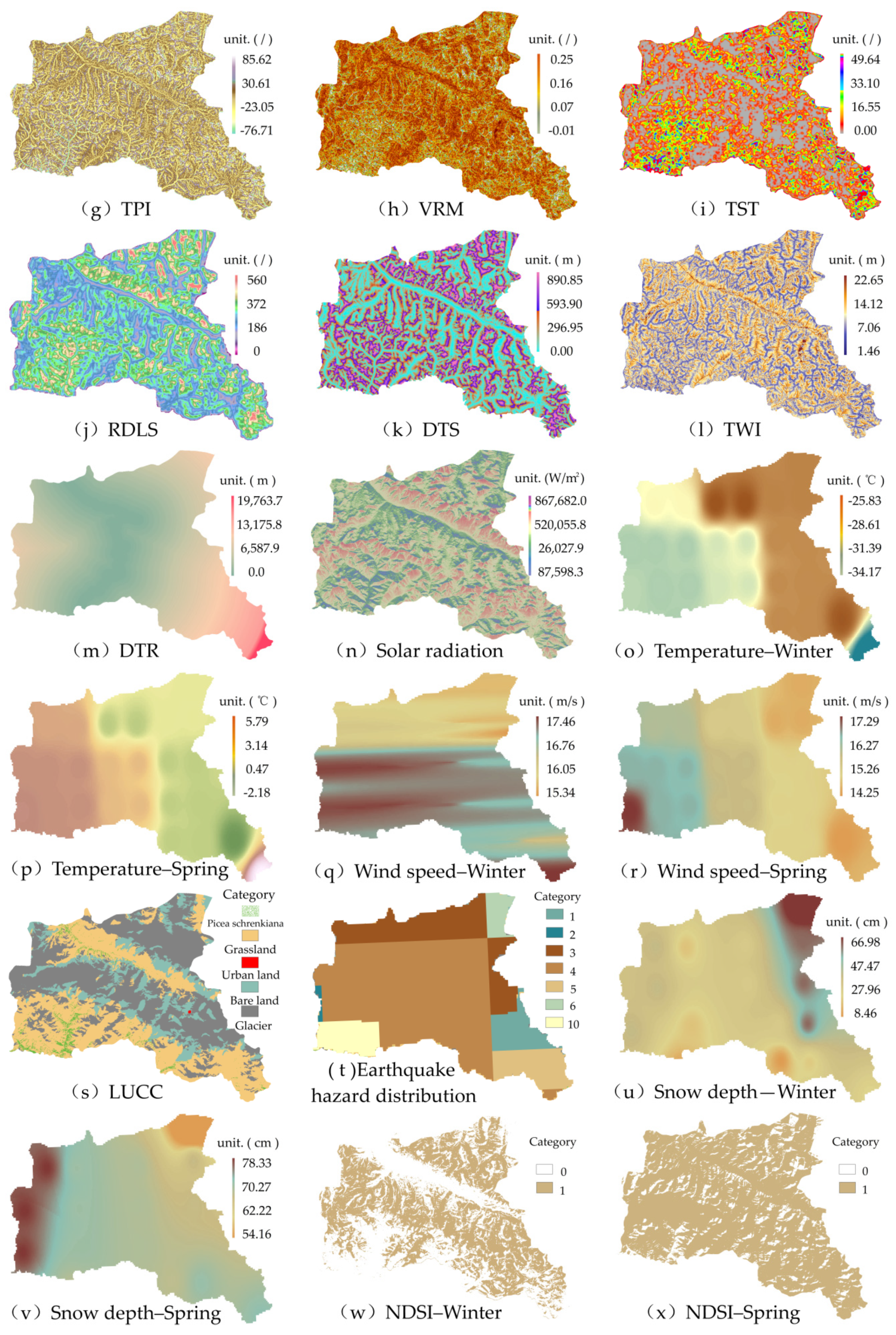
Years of field research have revealed that the occurrence of avalanches is mainly affected by terrain, weather, vegetation cover and snowfall. In this study, the terrain factors (Figure 6a–n) mainly included elevation, slope, aspect, plane curvature, profile curvature, terrain ruggedness index (TRI), topographic position index (TPI), vector ruggedness measure (VRM), terrain surface texture (TST), relief degree of land surface (RDLS), distance to stream (DTS), topographic wetness index (TWI), distance to road (DTR) and solar radiation, which were derived from analysis of the Digital Elevation Model (DEM) of the Advanced Land-Observing Satellite (ALOS). The spatial resolution was 12.5 m. The meteorological indicators—data on temperature and wind speed (Figure 6o–r)—were obtained from weather stations. The ground cover data (Figure 6s) were derived from land-use/-cover change (LUCC) in 2020, released by Professor Gong Peng [36] and his team from Tsinghua University, China. The spatial resolution was 10 m. Correlation indexes of crustal movement (Figure 6t) were derived from the raster data of the earthquake disaster distribution-peak ground acceleration (pga) published by NASA’s Earth-Observing System Data and Information System (EOSDIS). Snow depth (Figure 6u,v) was derived from the data in meteorological stations.

3.2.1. Topographic Factors

Elevation

According to the results of avalanche studies and field investigations, the area with an altitude of 2000–3500 m is prone to avalanches. Therefore, applying the elevation factor can highlight the vertical distribution of avalanche hazard in space.

Slope

Avalanches are sensitive to changes in the slope angle. However, an avalanche can only be released when the dip angle reaches a certain value (25–45°). When the dip angle exceeds 45°, slopes are less prone to avalanches because snow cannot be kept and piled up [37]. From a mechanical point of view, the interaction between the slope support force, friction force and gravity will affect the stress distribution of the snow layer on the slope, thus determining the avalanche hazard.

Aspect

The difference in solar radiation received by different slopes affects the thermal state of the snow layers and the metamorphic process. Therefore, the avalanche hazard varies from slope to slope.

Plane and Profile Curvature

The vertical and horizontal components of curvature are called plane curvature and profile curvature, respectively. Plane curvature refers to the degree of bending and the variation of the surface along the horizontal direction, which mainly determines whether the avalanche debris will be in convergence or dispersion when it is transferred in space. A positive plane curvature value represents a topographic bulge (such as a ridge) in which avalanche debris will flow to other areas; a negative value represents a topographic depression (such as a trench) in which avalanche debris will flow. Thus, a negative plane curvature value corresponds to a higher avalanche hazard level.
The profile curvature carves out the complexity of the concave and convex morphology change in the slope, which mainly affects the velocity of the avalanche debris erosion and braking. A positive section curvature value indicates a higher velocity of avalanche debris, and therefore, a higher hazard. Avalanche debris moving into the negative zone will be slowed down, thus representing a lower avalanche hazard.

TRI

TRI is used to describe the undulation degree of local terrain [38]. The value of a flat area is 0, and a positive value is used to describe the steepness of slopes. The closer TRI to 0, the lower the avalanche hazard.

TPI

TPI is an indicator that describes local elevation. If TRI is greater than 0, the central point is higher than the average surrounding elevation. If TRI is less than 0, the elevation value of the centre is lower than the mean of the elevation of the surrounding areas. Specifically, positive and negative values respond to ridge and valley topography, respectively; thus, they determine the impact force of avalanche debris. A value of zero (0) is a low avalanche hazard. Ridges, side slopes that connect valleys and areas where ridges meet valleys are areas of high avalanche hazard.

VRM

VRM quantifies the ruggedness of the snow layer by measuring the dispersion of the vectors perpendicular to the surface. As the value of VRM deviates from 0, the stress of the snow layer increases accordingly. Otherwise, it means that the snow layer becomes more unstable. Thus, areas with low values for VRM values are associated with high avalanche hazard.

TST

TST is one of the main parameters characterising geomorphic development. It quantifies the similarities and the differences in terrains. Areas with larger surface texture can better provide mechanical support for shallow snow, thus stabilising it. Avalanches are only triggered when the accumulation of snow exceeds the bearing capacity of the disaster-pregnant environment, thus affecting the hazard of avalanches.

RDLS

In this study, RDLS was used to quantify the geomorphic types that are described and the degree of surface cutting with the maximum elevation difference within a 3 × 3 grid [39]. The terrain of the study area was mainly undulating mountains and valleys in the mountain chain. The statistical results show that avalanches mostly occur in undulating mountains (70–500 m).

DTS

DTS describes the spatial heterogeneity of channel distribution. Hydrological processes near river channels are frequent and strong, which will change the characteristics and stability of snow on the slope areas. Generally speaking, the closer the snow to the river, the worse its stability, and the greater the hazard of avalanches.

TWI

TWI represents the humidity conditions and spatial distribution of avalanches. A high TWI value highlights that the areas with the potential for avalanche movement have a high avalanche hazard.

DTR

DTR describes the distance between a location in an area and a road. In avalanche disaster in the area investigated in this study, the road was the main disaster-bearing body, so the closer the area to the road, the higher its hazard level. Furthermore, due to pending road construction in the study area, the stability of side slopes in some of the areas was destroyed, resulting in increased avalanche hazard along the road.

Solar Radiation

Snow is preserved in areas with low solar radiation values, providing an abundant material base for triggering avalanches. However, the structure of the snow layer is tight and uniform, and the hazard of avalanche is low. In a region with a higher solar radiation value, the snow layer has a complex process of temperature gradient metamorphism, isothermal metamorphism and ablation-freezing metamorphism, so the structure of the snow layer is weak, which puts it at a greater hazard of avalanches.

3.2.2. Meteorological Factors

Temperature

Temperature is one of the dynamic factors affecting the hazard of avalanches. On the one hand, the dynamic effect lies in temperature fluctuations in a low-temperature environment, creating more avalanche material, which gradually leads to a high avalanche hazard. On the other hand, the temperature difference between day and night repeatedly freezes and thaws snow grains, which evolve into loose, large ice crystals and weaken the snow layer, which further increases the hazard. The temperature data in this study were obtained from daily data recorded by meteorological stations. In view of the large daily temperature difference in the study area, the mode of the temperature data was selected as the source data for the inverse distance weight interpolation.

Wind Speed

When the drag force of the wind is sufficient to break the adhesion and gravity between the snow grains, the snow layer breaks off the slope and triggers an avalanche [40]. Thus, stronger winds mean higher levels of avalanche hazard. In this study, the raster data of wind speed was generated by inverse distance weight interpolation after taking the meteorological station’s maximum value of daily wind speed data.

3.2.3. LUCC

To some extent, LUCC influences the distribution of avalanche hazard. For example, in avalanche terrain, trees such as Picea schrenkiana, J. pudosabina, and B. tianshan schanica with high canopy density, can intercept snowfall (about 270 mm), attenuate wind speed and stop avalanches. They are natural, ecological security barriers, ensuring a low avalanche hazard in the area. The low meadow growing in the disaster-pregnant body can effectively store up the snow accumulation in the early stage of the snowfall. However, when the snow depth exceeds the height of the meadow, these meadows will not be able to prevent the further development of avalanches. Therefore, such areas have a relatively high avalanche hazard. Under the same trigger conditions, bare ground has a higher avalanche hazard than grassland. Generally, flat, open agricultural land is not subject to avalanche hazard. The construction land, which becomes the disaster-bearing body, is in the high-hazard area.

3.2.4. Earthquake Hazard Distributions

An earthquake is the main internal driving force of surface disturbance, so it is a triggering factor of avalanches as well. Seismic wave energy can affect the avalanche hazard by lifting, dislocating, breaking or shaking the disaster-pregnant body, disrupting the balance of forces between the snow layer and the surface; this can trigger avalanches, thus affecting avalanche hazard. Raster data published by EOSDIS was used to characterise the relative distribution and frequency of earthquakes in Taldasha. To identify earthquake hot spots, pga values less of than 2 m/s in the grid were removed, and the total number of other grids was divided into deciles, with 10 representing the highest importance. In this study, high pga values are associated with high hazard.

3.2.5. Snow-Related Variables

Snow Depth

Based on years of observation data, when the depth of snow in the disaster-pregnant body reaches 40 cm, the local potential avalanche hazard must be considered, and when the snow depth of the avalanche terrain exceeds 70 cm, it is very likely to become a high-hazard area [28]. Therefore, spatial differences in snow depth directly lead to significant differences in avalanche hazard levels. At the same time, the single-peak variation of snow depth within a year in the study area makes snow depth a highly dynamic factor that affects the avalanche hazard and is a key factor that makes avalanche hazard appear to be seasonal. The snow depth raster data used in this study were also derived from the daily data of meteorological stations, which were interpolated by the inverse distance weight method after taking the maximum value.

NDSI

NDSI is a controlling factor for avalanche hazard. A value of 0 means no avalanche hazard, and the closer the value to 1, the more likely the hazard will be higher. The NDSI data came from the MOD10A2 eight-day synthetic snow cover data product of the Moderate Resolution Imaging Spectroradiometer (MODIS) satellite. The temporal and spatial resolutions were 8 d and 500 m, respectively, spanning approximately the same time period as the weather station data. The orbital number covering the study area was h24v04. A total of 22 images were collected, and MRT (MODIS Reprojection Tool) software was used for mosaic, reprojection and format conversion of the images. Then, the monthly NDSI data products were synthesised using the maximum value (Figure 6w,x).
The projected coordinates of the above-mentioned primary selected features and control factors were WGS84. The resolution was uniformly resampled to 500 m. The initial data set generated was processed without dimensions using range standardisation.

3.3. Methodology

3.3.1. Multicollinearity

Multicollinearity occurs when there are two or more independent variables that have a high correlation among themselves, leading to distorted or inaccurate avalanche hazard estimates. In this study, Variance Inflation Factor (VIF) was used to detect multicollinearity [41]. In the VIF method, each feature is identified and regressed against all of the other features [42]. For each regression, the factor is calculated as:
V I F = 1 1 R i 2
where R2 is the coefficient of determination in the linear regression, reflecting the extent to which the independent variable can be described by other variables. The value of VIF starts at 1 and has no upper limit. A value of 1 indicates that the independent variable is not associated with other variables. A VIF value greater than 10 indicates serious multicollinearity between the variables and corrective measures should be taken. Tolerance (TOL) is the reciprocal value of VIF. The smaller the TOL, the more serious the multicollinearity.

3.3.2. Feature Selection

Relief-F (F refers to the sixth algorithm variation [from A to F] proposed by Kononenko) is a well-known filtering feature-weight method. A related statistical vector is designed to measure the importance of features [43]. Assuming that the samples in the initial feature data set D are from ∣y∣ categories, then the component of the relevant statistical vector corresponding to the attribute j is:
δ j = i d i f f ( x i j , x i j , n h ) 2 + l k ( p l × d i f f ( x i j , l , n m ) 2 )
Among them, xi,nh and xi,l,nh are the nearest hits and nearest misses of the example xi found in each sample within and outside of category k, respectively. If the distance between the former and xi is small, it indicates that attribute j is beneficial for distinguishing the samples and should be retained. Otherwise, attribute j plays a negative role and should be removed. Pl is the proportion of type l samples in data set D.

3.3.3. Mann–Whitney U Test

In this study, the Mann–Whitney U test was used to detect whether the safe samples were mixed with the hazard samples [44]. The Mann–Whitney U test divides the test results of the two groups of test samples into two types: the population of the two sample data sets is the same (H0) and the population of the two sample data sets is not the same (H1).
The following steps are used. First, the two types of samples are mixed and then arranged in ascending order to identify the rank corresponding to each. In the next step, the average of the ranks of various samples ( W ¯ x and W ¯ y) is obtained and the gaps are compared. If the gap is large, the null hypothesis (H0) is likely to be invalid. Then, the number of ranks of each hazard sample greater than the rank of the safety sample (Uxy) is calculated and the number of ranks of each safety sample greater than the rank of the hazard sample (Uyx) is also calculated. If there is a big difference between Uxy and Uyx, the null hypothesis is likely to be invalid. Next, the Mann–Whitney U statistic (Formula (3)) is calculated based on Uxy and Uyx. Finally, the p value of a statistic is computed. If p < α (α is the significance level, α = 0.05), H0 is rejected, indicating that both samples are pure and statistically significant.
Mann–Whitney U statistics are defined as:
U = W k ( k + 1 ) 2
Given that k, the number of sample groups, corresponds to W (test statistic).

3.3.4. SVM

SVM is based on the principle of minimum structural hazard and has good generalisation capability. Its core idea is to find a hyperplane with the best tolerance in the sample space based on the training set, to divide the samples of different categories [45] and ensure that the classification results are robust.
The SVM algorithm requires a small sample size and can solve nonlinear high-dimensional problems. To achieve linear inseparability, the SVM algorithm needs to introduce a kernel function to project data from low dimensional space to the high dimensional space. Commonly used kernel functions include linear kernel functions, polynomial kernel functions and radial basis kernel functions (RBF). When different kernel functions are used, the form of SVM is also different.
The applicability of the kernel function is determined by the penalty factor C and the kernel function parameter g in the SVM model [46]. C controls the complexity and generalisability of the model, and g determines the range and width of the input space. If C is too large or too small, this will lead to over-fitting or under-learning. An inappropriate g value will result in insufficient model accuracy or introduce errors.

3.3.5. RF

RF is an integrated learning algorithm based on multiple decision trees. There is no relationship between each decision tree in the forest, and the final output of the model is jointly determined by each decision tree in the forest.
RF uses n decision trees to classify, and the differences between classification models are increased by constructing different training sets. The bootstrap method is used to randomly extract K training sets from the original data set, and then a forest composed of K CART decision trees is generated. During the growth of each tree, m (m ≤ M) split-point features are randomly selected from all the characteristic variables (M). According to the Gini coefficient minimum principle, the optimal feature is selected for internal node branch, so that each tree can grow fully without pruning. Finally, the results predicted by K decision trees are collected to determine the category of the new samples [47].

3.3.6. KNN

The KNN algorithm is a general approximator of the relationship between a set of data. The principle is as follows: If a sample to be classified has k most similar samples in the feature space, most of which belong to a certain category, the sample also belongs to this category [48].
The most important parameter in KNN is the determination of the k value. If the value of k is too large, the k neighbours of the object to be classified are very likely to include other types of data objects. Moreover, the number of data objects in a certain category may exceed the number of data objects in the actual category of the object to be classified. These circumstances will lead to the inaccurate category labelling of the objects to be classified. If the k value is too small, it may be affected by noise data.

3.4. Performance Verification of the Model

Receiver operating characteristic (ROC) curve, Matthews correlation coefficient (MCC), overall accuracy (OA), frequency of misses (FOM), probability of false detection (POFD) and frequency bias (FB) indicators are used to objectively evaluate and compare the performance of models.

3.4.1. ROC

The ROC curve takes the true positive rate (TPR) as the vertical axis and the false positive rate (FPR) as the horizontal axis.
T P R = T P T P + F N
F P R = F P T N + F P
True positive (TP)refers to the number of hazard pixels correctly defined, false negative (FN) refers to the number of hazard pixels incorrectly judged as safe pixels, true negative (TN) refers to the number of safe pixels accurately determined, false positive (FP) is the number of safe pixels incorrectly defined as hazard pixels. When the ROC curve of one model is completely covered by the curve of the other classifier, the latter has better performance. If the curves cross, the area under curve (AUC) is used as the criterion.
AUC = 1 2 i = 1 m 1 ( x i + 1 x i ) ( y i + y i + 1 )
Here, m is the number of samples, and (x, y) is the coordinate point in ROC.

3.4.2. Statistical Indicators

MCC is a relatively balanced and the most informative single score for building binary classifiers to predict quality in the context of a confusion matrix, which returns the value of [−1, 1]. Coefficient +1 means perfect prediction, 0 means no better than random prediction, and −1 means complete inconsistency between prediction and observation [49].
M C C = T P × T N F P × F N ( T P + F P ) ( T P + F N ) ( T N + F P ) ( T N + F N )
OA quantifies the ability of the model to determine the attribution of the pixels. It ranges from 0 to 1. A perfect score is 1.
O A = T P + T N T N + F N + T P + F P
FOM quantifies the rate at which hazard pixels are missed.
F O M = F P T P + F P
POFD is a measure of inaccuracy with respect to the observations; it provides a measure of the extent to which the forecasts provide a false warning for the occurrence of an event. FOM and POFD vary from 0 to 1; values near zero are better than other values.
P O F D = F N F N + T N
The value of FB ranges from 0 to infinity. If it is over 1, it indicates that the model has widespread misjudgment; if it is less than 0, it indicates that missed judgment is more common.
F B = T P + F P T P + F N

3.5. Experimental Design

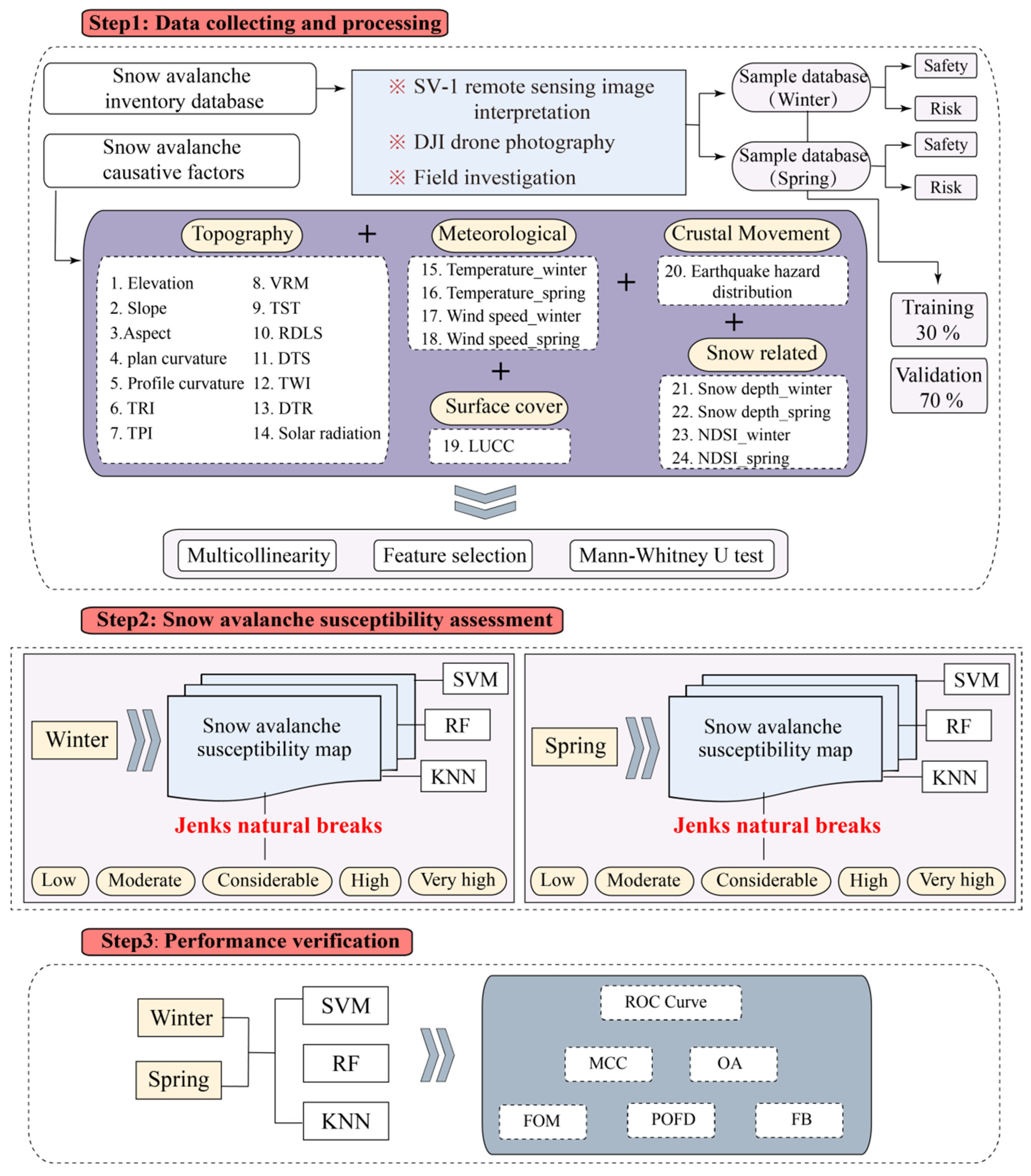
The following steps are used to build a framework for an avalanche hazard assessment scheme (Figure 7).
  • Collect complete and accurate avalanche inventory in Taldasha and establish a sample database through the integrated avalanche survey network of “space–air–ground”. Establish a hazard driving-factor database related to topography, meteorology, surface cover, crustal dynamics and snow conditions according to the local avalanche disaster-pregnant environment.
  • Optimise the introduced drivers, including multicollinearity analysis and relief-F, and use the Mann–Whitney U test to verify the purity of the safe samples and hazard samples. Establish training samples and testing samples for spring and winter, respectively, on the basis of the above optimisation of the causative factors.
  • Apply SVM, RF and KNN algorithms, respectively, to learn the samples. Build models with appropriate accuracy, and evaluate the avalanche hazard of Taldasha in winter and spring.
  • Evaluate and compare the performance of the models.

4. Results

4.1. Avalanche Susceptibility Modeling

4.1.1. Multicollinearity Analysis

As seen in Table 3, there is no serious multicollinearity in the causative factors in winter and spring (VIF < 10 and TOL > 0.100).
In general, the VIF value of the above incentives ranges from 1.042 to 5.424, and the TOL is much greater than 0.100. Among them, only the VIF value of temperature in spring is slightly greater than 5, but it is still far less than 10. In conclusion, there is no multicollinearity in the causative factors in winter and spring.
With the control group established the season-based consistency of model efficiency was measured. The hazard and safety samples consisted of set of samples collected in spring and winter, respectively. In particular, the value selection falls into the average of air temperature and wind speed in the avalanche, and the maximum cumulative snow depth over the span of a year. In terms of multicollinearity analysis, the wind speed VIF in the control group is >5 (VIF = 6.808), but within 10 and TOL > 0.100; thus, there is no severe multicollinearity. The remaining variables in the control group were 1.028 ≤ VIF ≤ 3.152 and 0.317 ≤ TOL ≤ 0.973. Overall, there was no severe multicollinearity in variables of the control group.

4.1.2. Elimination of the Less Important Causative Factors

Table 4 shows the weights of the causative factors obtained by averaging the weights obtained by the relief-F algorithm, iteratively, 20 times. In summary, the contribution rate of each causative factor is very different in winter, spring and the control group.

4.1.3. Difference between Hazard Samples and Safety Samples

Table 5 shows the difference between the hazard samples and safety samples based on the Mann–Whitney U test results. The p values in the table are significantly less than 0.050, indicating that the U-test for incentives in winter, spring and the control group rejected the H0 hypothesis. Thus, there are obvious differences in all the variables for the hazard samples and safety samples selected in this study.

4.2. Avalanche Susceptibility Cartographic Representation

4.2.1. Parameterisation Scheme of Avalanche hazard Assessment Model

The performance of the SVM model largely depends on whether the selected kernel function is appropriate. Table 6 lists the parameters of the SVM model. The results show that when the performance of the SVM model for winter, spring and the control group is good, the AUC value can reach 0.995 (the kernel function is RBF, C = 1, g = 0.5).
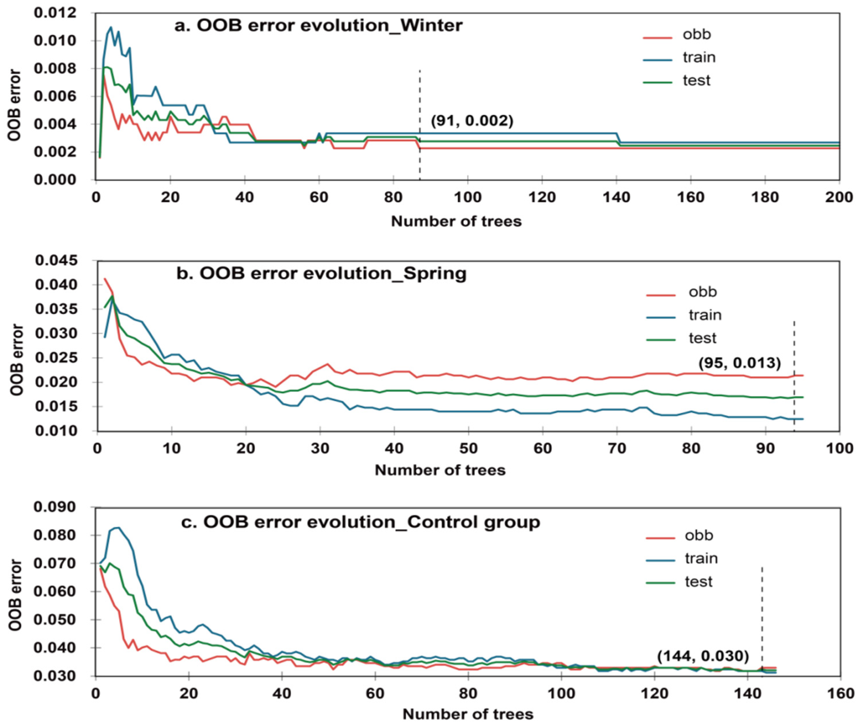
The key to ensuring the performance of the RF model is the setting of the k variable (number of trees). Out-of-bag (OOB) error is an unbiased estimation of the RF generalisation error [50]. In this study, the OOB error corresponding to each k value was calculated in 20 steps.
The results show that when k is 91 in winter, the OOB error is the smallest (OOB error = 0.002) and becomes stable (Figure 8a). Therefore, when using the RF model to evaluate the avalanche hazard in winter, the optimal k value is 91. Similarly, the optimal k values of spring (Figure 8b) and the control group (Figure 8c) are 95 and 144, respectively, and the corresponding minimum OOB error values are 0.013 and 0.030, respectively.
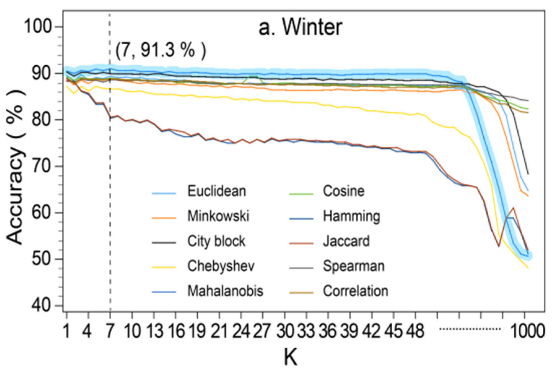
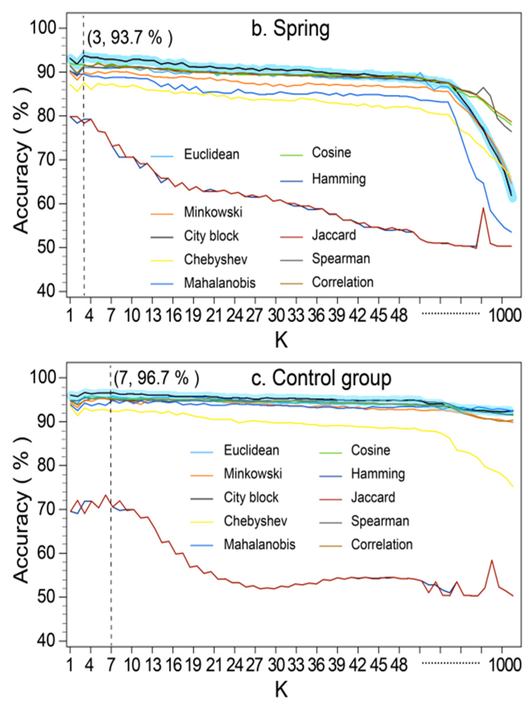
The KNN model-based hyper parameter is composed of k and the measurement of distance. In this study, 10 distance measurement standards were tested—Euclidean, Minkowski, city-block, Chebyshev, Mahalanobis, cosine, hamming, Jaccard, Spearman and correlation—to accurately find the types of distance measures that can maximise the performance of the KNN model.
The results show that, in the winter case (Figure 9a), when k = 7 and the distance measure is Mahalanobis, the accuracy of the KNN model is the highest at 0.913. In the spring case (Figure 9b) and the control group case (Figure 9c), when the distance measure is city block and k values are 3 and 7, respectively, the model presents the best accuracy with 0.937 and 0.967, respectively. Therefore, 7, 3 and 7 are the best choice for the KNN model to evaluate the avalanche hazard in winter, spring and the control group, respectively, and the corresponding distance measures are Mahalanobis, city block and city block.

4.2.2. Spatial Characteristics of Avalanche Hazard

Based on the avalanche hazard classification standard [51] of the European Avalanche Warning Services (EAWS), this study used the Jenks natural breaks method [52] to divide the hazard into five levels: low, moderate, considerable, high and very high, respectively.
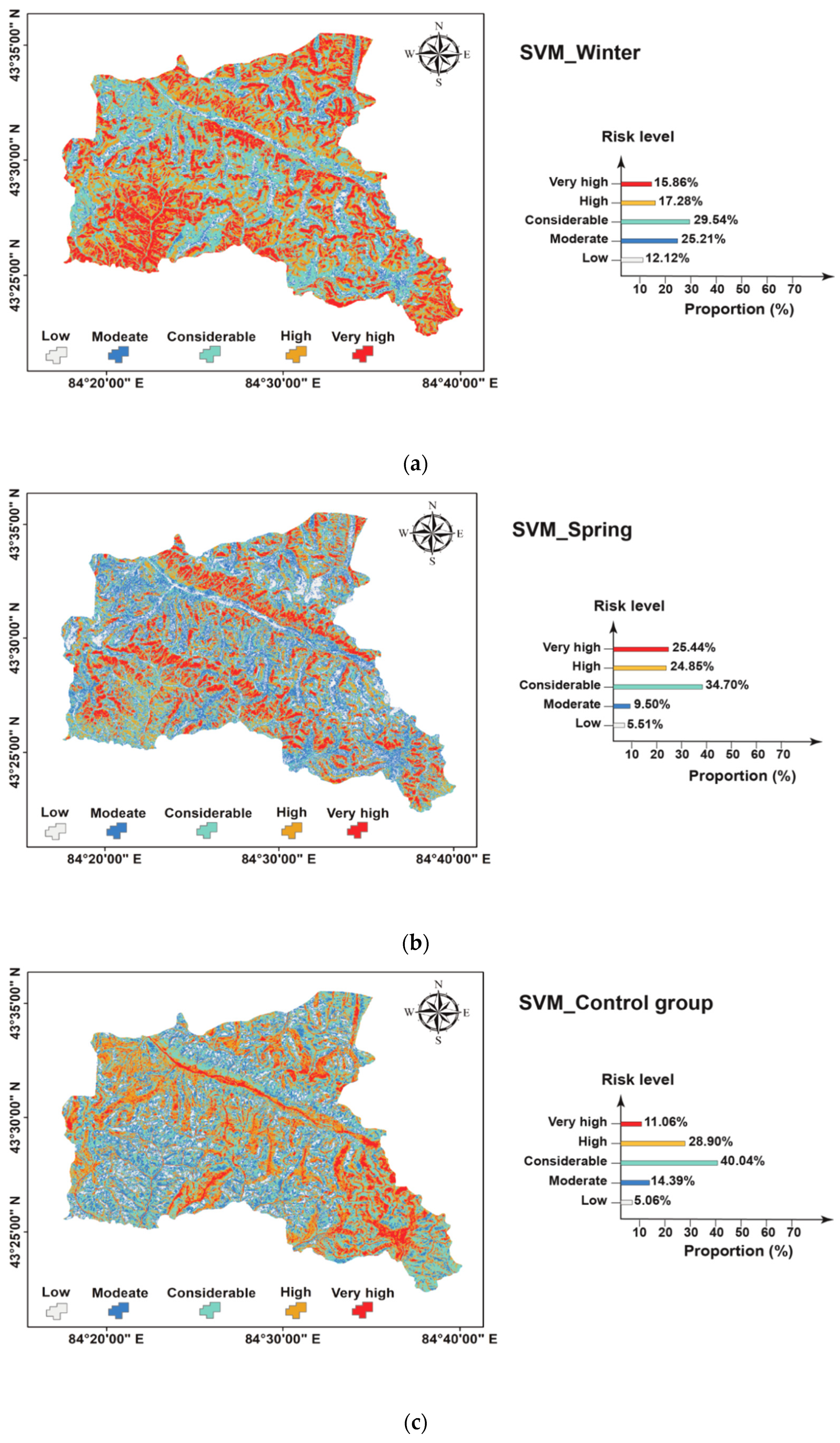
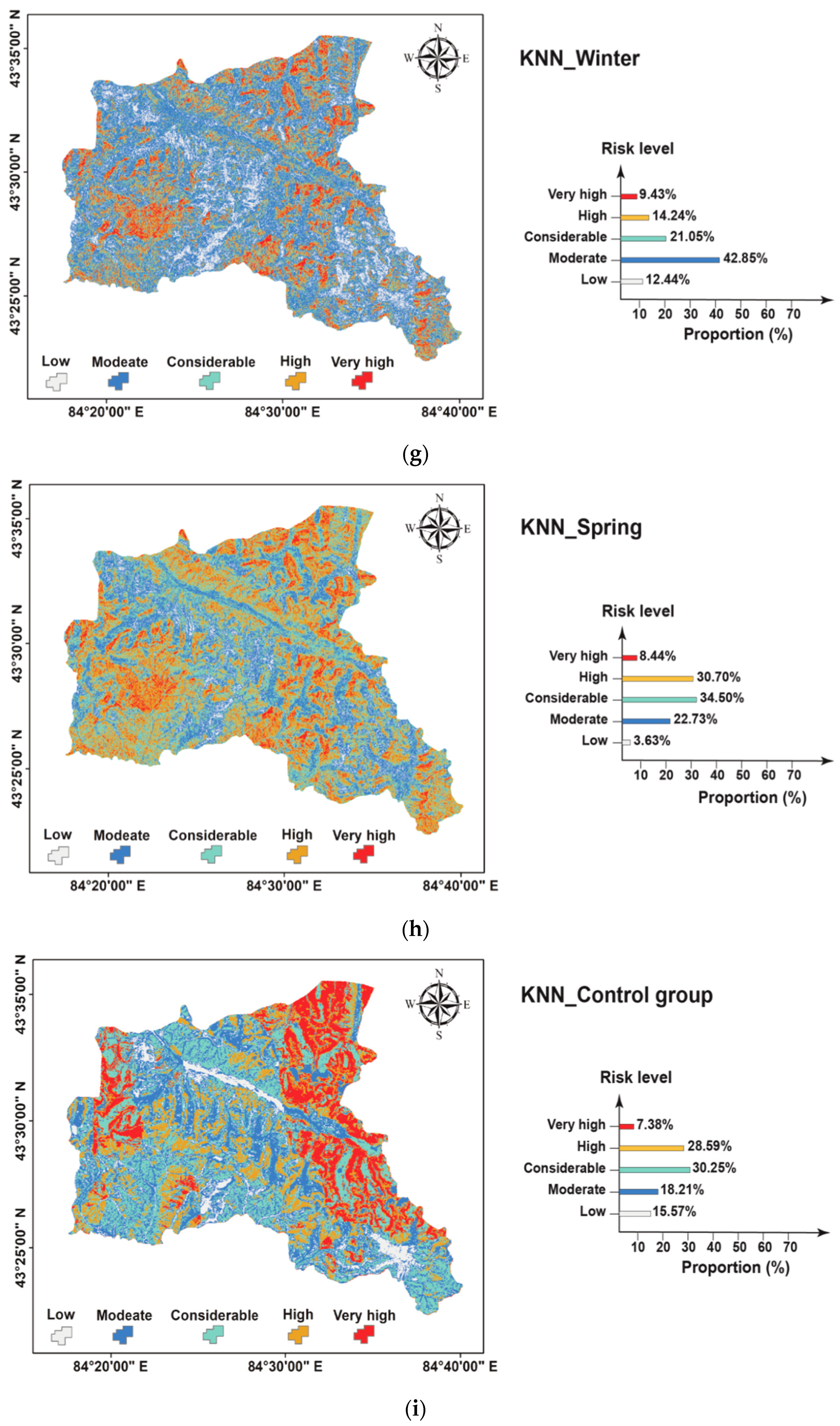
As seen in Figure 10, the hazard distribution obtained by the SVM model, RF model and KNN model has obvious and consistent topographic differentiation. Specifically, whether in winter or spring, the low-hazard area is mainly distributed in the middle, while the highly avalanche-prone area is in the southwest. Avalanche hazard in the northeast is overlapped with multiple levels. In detail, the low-hazard areas are mainly distributed in flat areas and areas with open plains and peaks. The slope in this area does not exceed 22.66° and the altitude ranges from 2091–3000 m. The land cover in the region is mainly low mountain meadow. The moderate avalanche hazard is widely distributed throughout the study area and mostly in piedmont, with an altitude ranging from 3000–3500 m. In particular, moderate avalanche hazard occurs in the areas with more snow days. Considerable avalanche hazard is mostly distributed at the ridge, including slope-connected valleys or ridge-valley junctions. High avalanche hazard is mainly distributed in the south-western part of the study area. The terrain of this area mainly consists of trenches and valleys that can easily accommodate snow, with a snow depth of 54–71 cm and a slope of 30°–40°. Very high hazard is mainly distributed in the mountainous and canyon areas with a rough surface and deep cutting in the southern part of the study area.
However, in the control group (Figure 10c,j,i), the spatial distribution of avalanche hazard has no obvious regular characteristics. For example, in the northeast, the avalanche hazard obtained by the SVM model is mainly considerable, while the hazard RF model shows an overlapping of hazard levels of moderate, considerable, high and very high. Moreover, the avalanche hazard obtained by the KNN model is mainly very high in this area. The disordered results also existed in the south-eastern and north-western parts of the study area. On the whole, in the control group, although low- and moderate-hazard levels have the same topographic distribution characteristics (mainly distributed in the flat and open piedmont alluvial plain), it was not possible to determine the topographic distribution characteristics of the avalanche hazards of the other levels.

4.2.3. Seasonal Characteristics of Avalanche hazard

As seen in Figure 10, there are seasonal differences in the avalanche hazard distribution in winter and spring. For example, according to the avalanche hazard distribution results presented by the SVM model, the avalanche hazard in winter (Figure 10a) is mainly at the considerable level, accounting for 29.54%. In descending order, the avalanche hazards of moderate, high, very high and low are 25.21%, 17.28%, 15.86% and 12.12%, respectively, and the proportion of the latter three is similar. In spring (Figure 10b), with the significant decrease in the proportion of low and moderate hazard, the proportion of considerable, high and very high avalanche hazards increases. In other words, during the transition from winter to spring, the dynamic change characteristics of avalanche hazard can be described as a low-level hazard and a medium–low-level hazard evolving into a medium–high-level hazard and a high-level hazard by a wide margin.
The RF model winter avalanche hazard distribution (Figure 10d) is mainly at the considerable hazard level (33.24%). The low (14.43%), moderate (15.11%), high (19.37%) and very high (17.85%) levels of hazard are almost the same. After the spring season (Figure 10e), the proportion of low and considerable hazards decreases significantly; in fact, the reduction in considerable hazard is significant (8.72%). Accordingly, the high-level hazard area increases from 19.37% in winter to 32.81% in spring. The moderate- and very high-level hazards were relatively stable in the seasonal changes. Therefore, the seasonal difference in avalanche hazard level can be described as the gradual evolution from a low– and medium–high level to a high level.
In the KNN model, the winter avalanche hazard (Figure 10g) is mainly at a moderate level, about 42.85%, followed by the considerable hazard level (21.05%). The high hazard level is 14.24%. The proportion of the other hazard levels is between 9% and 12%. In the spring (Figure 10h), the most significant change is the dramatic decline in the moderate hazard level (20.12%) and the low hazard level (8.81%), and the corresponding increase in the considerable hazard level (13.45%) and the high hazard level (16.46%). There is no obvious seasonal change in the proportion of the very high hazard level. Thus, the seasonal variation characteristics of avalanche hazard, in this case, are mainly the evolution from the low-, medium- and low-level hazard to medium- and high-level hazard.
In the control group (Figure 10c,f,i), the avalanche hazard presented by the models is always medium and high. Specifically, the avalanche hazards assessed by the SVM model, RF model and KNN model are mainly considerable hazard levels, accounting for 40.04%, 34.78% and 30.25%, respectively. In conclusion, the control group results only represent the general hazard level throughout the entire avalanche period. It is worth noting that the control group could not show the seasonal efficiency of the model and the drastic change in avalanche hazard based on the season.

4.3. Model Performance Verification and Comparison

4.3.1. Using ROC

ROC is an important index for evaluating model performance. By analysing the ROC curves of the models, it is found that the performance of the models is: RF model > SVM model > KNN model, which is consistent in season.
Figure 11a indicates that the RF model had the best performance in evaluating avalanche hazard in winter (AUC = 0.88). The second-best performance was delivered by the SVM model, whose AUC value (0.86) is slightly lower than the RF model by 0.02. The performance of the KNN model was not as good (AUC = 0.84). In the spring case (Figure 11b), the order of model performance is: the RF model (AUC = 0.91), the SVM model (AUC = 0.85) and the KNN model (AUC = 0.81). In the control group (Figure 11c), the comparison results of model performance are consistent with the results for winter and spring. The AUC values are 0.78 (RF model), 0.74 (SVM model) and 0.72 (KNN model), respectively, but with relatively low reliability of prediction results.
Based on the seasonal performance analysis of model efficiency, the RF model has excellent performance in winter. The difference in the AUC value in the spring season is only 0.03. The SVM model and KNN model have a more satisfactory performance in the spring cases. The seasonal differences in their AUC values are only 0.01 and 0.03, respectively. In view of the small seasonal difference in the AUC value of the model, it is considered that the model efficiency is consistent in season.

4.3.2. Using Accuracy Statistics

Based on the evaluation of model performance using various indicators (Table 7), the RF model performed the best, followed by the SVM model and the KNN model.
Specifically, in winter cases, the MCC and OA values of the RF model are closest to 1, 0.965 and 0.935, respectively. The FOM value (0.111) and POFD value (0.014) of that model are closest to 0. The FB value of the RF model is between 0 and 1, indicating that there is no common misjudgment or omission. Therefore, it is the most superior model in this case. The MCC, OA, FOM and POFD values of the SVM model and KNN model are relatively similar. However, since the FB of the KNN model is 1.011, it indicates that there is a high misjudgment rate in the predicted avalanche hazard, resulting in inferior performance than the SVM model.
In the spring case, the RF model performance is still the best. The MCC, OA, FOM and POFD values of the SVM model and the KNN model are close. However, combined with FB (0.600 and 1.218, respectively), it is not difficult to judge that the performance of the KNN model is slightly inferior due to the high rate of misjudgment.
The overall performances of the SVM model, RF model and KNN models are not as good in the control group as in winter or spring cases. In the control group, the RF model has higher MCC and OA values and lower FOM and POFD values, so its performance is slightly better. The FB values of the SVM model and KNN model are 1.160 and 1.601, respectively, indicating that there is a high misjudgment rate in the model, and the misjudgment rate of the KNN model is relatively higher.
Overall, the accuracy index of each group of cases shows that the prediction accuracy of the models in the control group is lower than the prediction accuracy of the models in spring and winter. The performance of the RF model is excellent, followed by the SVM model. The performance of the KNN model is slightly poor.

5. Discussion

5.1. Model Performance

5.1.1. Influence of Optimised Explanatory Variables on Model Accuracy

Based on existing research results reported in studies on the mechanism of avalanches, the factors influencing avalanche hazard include topography, meteorology and snow characteristics [15]. In some areas, these factors also include anthropogenic and crustal movement [53]. These studies usually classify topographic factors as static variables; they take the meteorological and snow characteristics as driving factors and they quantify the weights of inducing the factors in global avalanche prone areas, such as Hindu Kush, the West Himalayas and the Alps, at an interannual scale. The results show that slope and solar radiation are the most important explanatory variables among of the types of topographic variables [4], and precipitation and air temperature are the most important driving factors among the various meteorological factors [30]. Some statistical models also predict avalanche hazard under current meteorological conditions by statistically correlating the values of the meteorological elements during avalanches, historically, with the avalanche probability density values (0–1) [24]. The results show that the avalanche hazard in a region is related to air temperature and shortwave radiation [54]. When the daily average temperature gradually reaches 2.5–4 °C and the daily average shortwave radiation is 140–180 W/m2, the correlation degree is as high as 0.8. These results show that an avalanche is an elaborate nonlinear process involving the joint action of many factors [25]. Therefore, it is not sufficient to use a single explanatory variable or partial explanatory variables to predict avalanche hazard; more reliable results can only be obtained by the integration of topography, meteorology and snow characteristics. However, some studies have pointed out that an avalanche hazard assessment model with topographic, meteorological and snow characteristics [8,55] can still have a high false alarm rate (FAR > 0.784).
Based on the research cited above, the avalanche hazard model established in the present study departs from the comprehensive consideration of the interannual scale. It researches season-based avalanche hazard to reduce the impact of the uncertainty of the input variables on the accuracy of the model. The model constructed in this study covers all the related variables, as far as possible, by including topography, meteorology, surface cover, crustal movement and snow characteristics. Table 8, Table 9 and Table 10 show the impact of combining with multi-source heterogeneous variables on the performance of the SVM model, the RF model and the KNN model, respectively. The results show that whether in winter or spring, the gradual introduction of variables further improves the performance of the avalanche hazard assessment framework model developed in this study. This further validates the positive role of combining multi-source heterogeneous factors in the model to improve the reliability of the results. At the same time, when combined with the control group designed in this study, the avalanche hazard evaluated by the model has relatively low prediction accuracy. As a whole, the AUC value of the model is 0.09–0.13 lower than in the winter or spring cases. Moreover, the differences in the performance of the model in winter, spring and the control group show that it is meaningful to explore the seasonality of avalanche hazard. It confirms that in order to ensure that the model achieves the best performance, it is necessary to consider the seasonal differences in the nonlinear relationship variables.

5.1.2. Advantages of the Model Framework

The avalanche hazard assessment framework used in this study was developed by establishing a sample database, optimising the explanatory variables and selecting the algorithms. To establish the sample database, the large-capacity and high-precision avalanche inventory and sample data were obtained from the air–space–ground survey network. Based on the Mann–Whitney U test results, the hazard samples and safety samples were found to be completely different for all the variables. This conclusion effectively affirms the study’s effort to expand the category boundaries of the samples. At the same time, having enough pure samples avoids mixing noise into the model. However, some studies have used K-means clustering analysis to select samples. This method of distinguishing sample categories by data features and similarity will easily introduce noise caused by extreme conditions with the increase in sample size. The optimisation variable flow includes multicollinearity analysis and relief-F. In this study, the avalanche hazard explanatory variables were selected according to the local avalanche mechanism and previous experience. Multicollinearity analysis showed that there was no serious multicollinearity of the variables in winter, spring or the control group. This ensures the effectiveness of the selected variables in the interpretation of avalanche hazard and avoids redundancy. Relief-F was used to quantify the independent effect of each variable on avalanche hazard. In comparison to principal component analysis and the information entropy model, relief-F is not limited by data types and is not sensitive to the correlation between variables; thus, a more accurate factor weight is obtained. In fact, some studies have determined the weight of variables with the help of expert scoring methods [29]. However, when faced with a weight assignment task with fine requirements, or in the case of a lack of prior knowledge, the weight obtained by experts has a certain degree of human subjectivity. In comparison, the weight obtained in this study using the relief-F method is more objective.
For the selection of algorithms, this study chose a typical representative machine learning algorithm to describe the nonlinear relationship between the avalanche hazard and impact factors. Among them, SVM is a typical representative of a supervised classification algorithm with strong generalisation capability, and it is one of the most robust prediction methods. Previous studies have used SVM models to obtain avalanche susceptibility in northern Iran and landslide susceptibility in south-western China [47]. RF, which represents the level of integrated learning techniques, has also been used to assess avalanche hazards in the Zarrinehroud and Darvan basins of Iran [29]. KNN is a typical example of lazy learning. Some studies have applied KNN models to assess landslide hazard in north-western Jeddah in Saudi Arabia [56], and the Rangamati district in Bangladesh [57]. The results reported in those studies show that the SVM, RF and KNN algorithms are also suitable for evaluating avalanche hazard in high and cold mountain areas, and they highlight the advantages of a data-driven machine learning model in avalanche hazard assessment. In the SVM model, RF model and KNN model constructed in the present study, because the prediction result of the RF model is the mean value of a given number of decision trees, the optimal prediction accuracy is obtained without significantly increasing the operation time. Moreover, the performances of the SVM model, RF model and KNN model are excellent and consistent for both of the studied seasons (winter and spring). However, in the control group, the predictive value of the three models is relatively low.
It should be noted that although dynamic models, such as Rapid Mass Movement Simulation, can describe avalanche hazard based on quantitative avalanche destructive power [58], this method requires and relies heavily on specific input data [5,59]; moreover, it can only evaluate the hazard of avalanches in a single predefined path [10], so the efficiency is low.
Therefore, the avalanche hazard assessment framework based on machine learning can describe the nonlinear relationship between avalanche hazard and its impact factors more objectively, accurately and quickly than other models; thus, it is an effective scheme to address avalanche hazard assessment on a large scale.

5.2. Limitations

Based on previous research, insufficient or redundant explanatory variables will lead to the uncertainty of avalanche hazard assessment. Therefore, the present study evaluated avalanche hazard by optimising the explanatory variables of multi-source heterogeneity, and the AUC values of the models reached 0.81–0.91. Furthermore, the avalanche hazard assessment framework constructed in this study is objective, efficient and reliable, and it can be replicated and extended to other mountain areas that are affected by avalanches.
However, limited by the monitoring capability of the existing air–space–ground observation network, the meteorological and snow characteristics that were obtained cannot reflect the real-world situation of the surface area in detail. For example, the characteristics of snow cover and the spatial heterogeneity of meteorological elements in the western Tianshan Mountains in China are complex and changeable, so the grids of snow depth, temperature and wind speed used in this study cannot explain their spatial heterogeneity. At the same time, it is difficult to continuously monitor mechanical parameters, such as shear strength and Young’s modulus, which describe the vulnerability of the snow layer; therefore, they are not considered in this study. Based on our investigation of avalanche traces and avalanche landscape signs, it was found that there are disaster chains of avalanche-debris flow and landslide-snowmelt flood in the western Tianshan Mountains of China. The disaster-prone area in the mountains of this chain is similar, so it is susceptible to being misjudged.

6. Conclusions and Future Development

This study fills the gap of avalanche hazard assessment of dry–cold snow in the Tianshan continent of China by developing a hazard assessment scheme of the SVM model, RF model and KNN model that combines multi-source heterogeneous variables. After the models were compared and their performance was verified, the RF model with integrated learning had the best prediction accuracy.
The models used topography, meteorology, cover type, crustal movement and snow characteristics as the driving factors, and considered the differences in the avalanche hazard and dynamic changes between winter and spring. Moreover, the results show that seasonal assessment beyond the interannual scale can reduce the model uncertainties and the hazard tends, to develop into a high-level hazard during seasonal rotations.
The contribution rate of each causative factor is very different in winter and spring. In winter, it is mainly controlled by topographic variables and snow depth, and in spring, it is significantly affected by snow depth and temperature. The variables that determine the dynamic process of avalanche hazard are snow depth, DTR, temperature and LUCC. More importantly, considering seasonal differences in nonlinear relationship variables can drive the model to optimal performance.
Although optimisation of multi-source heterogeneous variables can improve the performance and overall accuracy of the model, the lack of more detailed snow characteristic data and mechanical element data limits the model’s accuracy. In follow-up research, it is important to improve the fine monitoring capability of the air–space–ground monitoring network and develop a hybrid model of a coupled physical model and machine learning, to achieve a more precise and accurate avalanche hazard assessment. In addition, it is necessary to emphasize the policy implications of avalanche hazard assessment, and promote the promulgation of relevant policies and regulations to scientifically regulate land use, construction of protection measures, avalanche education, and avalanche rescue in avalanche areas; this is necessary to improve avalanche governance capabilities and coordinate the development and safety of mountainous areas.

Author Contributions

All co-authors of this manuscript significantly contributed to all phases of the investigation. They contributed equally to the preparation, analysis, review and editing of this manuscript. All authors have read and agreed to the published version of the manuscript.

Funding

This research was funded by the National Natural Science Foundation of China (NSFC Grant No. 41901087), the Second Tibetan Plateau Scientific Expedition and Research program (2019QZKK010206) and the West Light Foundation of the Chinese Academy of Sciences (Grant No. 2018-XBQNXZ-B012).

Institutional Review Board Statement

Not applicable.

Informed Consent Statement

Not applicable.

Data Availability Statement

Not applicable.

Acknowledgments

We would like to thank my supervisor, Researcher Qing He, and the corresponding author, Associate Researcher Yang Liu, for providing important scientific guidance and equipment for avalanche survey and aeeseement research. We thank the editor-in-chief and anonymous reviewers for their useful feedback that improved this paper.

Conflicts of Interest

The authors declare no conflict of interest.

References

  1. Liu, Y.; Chen, X.; Qiu, Y.; Hao, J.; Yang, J.; Li, L. Mapping snow avalanche debris by object-based classification in moutainous regions from Sentinel-1 images and causative indices. Catena 2021, 206, 105559. [Google Scholar] [CrossRef]
  2. D’Aubeterre, G.; Favillier, A.; Mainieri, R.; Lopez, J.; Eckert, N.; Saulnier, M.; Peiry, J.; Stoffel, M.; Corona, C. Tree-ring reconstruction of snow avalanche activity: Does avalanche path selection matter? Sci. Total Environ. 2019, 684, 496–508. [Google Scholar] [CrossRef]
  3. Kumar, S.; Srivastava, P.K.; Snehmani; Bhatiya, S. Geospatial probabilistic modelling for release area mapping of snow avalanches. Cold Reg. Sci. Technol. 2019, 165, 102813. [Google Scholar] [CrossRef]
  4. Peitzsch, E.H.; Hendrikx, J.; Fagre, D.B. Terrain parameters of glide snow avalanches and a simple spatial glide snow avalanche model. Cold Reg. Sci. Technol. 2015, 120, 237–250. [Google Scholar] [CrossRef]
  5. Fischer, J.T. A novel approach to evaluate and compare computational snow avalanche simulation. Nat. Hazards Earth Syst. Sci. 2013, 13, 1655–1667. [Google Scholar] [CrossRef] [Green Version]
  6. Yariyan, P.; Avand, M.; Abbaspour, R.A.; Karami, M.; Tiefenbacher, J.P. GIS-based spatial modeling of snow avalanches using four novel ensemble models. Sci. Total Environ. 2020, 745, 141008. [Google Scholar] [CrossRef] [PubMed]
  7. Gądek, B.; Kaczka, R.J.; Rączkowska, Z.; Rojan, E.; Casteller, A.; Bebi, P. Snow avalanche activity in Żleb Żandarmerii in a time of climate change (Tatra Mts. Poland). Catena 2017, 158, 201–212. [Google Scholar] [CrossRef]
  8. Haraldsdóttir, S.H.; Ólafsson, H.; Durand, Y.; Giraud, G.; Mérindol, L. A system for prediction of avalanche hazard in the windy climate of Iceland. Ann. Glaciol. 2004, 38, 319–324. [Google Scholar] [CrossRef] [Green Version]
  9. Engeset, R.V.; Pfuhl, G.; Landr, M.; Mannberg, A.; Hetland, A. Communicating public avalanche warnings-what works? Nat. Hazards Earth Syst. Sci. 2018, 18, 2537–2559. [Google Scholar] [CrossRef] [Green Version]
  10. Gruber, U.; Bartelt, P. Snow avalanche hazard modelling of large areas using shallow water numerical methods and GIS. Environ. Model. Softw. 2007, 22, 1472–1481. [Google Scholar] [CrossRef]
  11. Prabhjot, K.; Jagdish, C.J.; Preeti, A. A multi-model decision support system (MM-DSS) for avalanche hazard prediction over North-West Himalaya. Nat. Hazards 2021, 110, 563–585. [Google Scholar] [CrossRef]
  12. Barbara, M. An ArcGIS Geo-Morphological Approach for Snow Avalanche Zoning and hazard Estimation in the Province of Bergamo. J. Geogr. Inf. Syst. 2017, 9, 83–97. [Google Scholar] [CrossRef] [Green Version]
  13. Aydin, A.; Eker, R. GIS-based snow avalanche hazard mapping: Bayburt-Așağı Dere catchment case. J. Environ. Biol. 2017, 38, 937–943. [Google Scholar] [CrossRef]
  14. Yariyan, P.; Omidvar, E.; Karami, M.; Cerdà, a.; Pham, Q.B.; Tiefenbacher, J.P. Evaluating novel hybrid models based on GIS for snow avalanche susceptibility mapping: A comparative study. Cold Reg. Sci. Technol. 2022, 194, 103453. [Google Scholar] [CrossRef]
  15. Parshad, R.; Srivastva, P.K.; Snehmani; Ganguly, S.; Kumar, S.; Ganju, A. Snow Avalanche Susceptibility Mapping using Remote Sensing and GIS in Nubra-Shyok Basin, Himalaya, India. Indian J. Sci. Technol. 2017, 10, 1–12. [Google Scholar] [CrossRef] [Green Version]
  16. Reichstein, M.; Camps-Valls, G.; Stevens, B.; Jung, M.; Denzler, J.; Carvalhais, N.; Prabhat. Deep learning and process understanding for data-driven Earth system science. Nature 2019, 566, 195–204. [Google Scholar] [CrossRef]
  17. Gall, J.; Yao, A.; Razavi, N.; Gool, L.V.; Lempitsky, V. Hough Forests for Object Detection, Tracking, and Action Recognition. IEEE Trans. Pattern Anal. Mach. Intell. 2011, 33, 2188–2202. [Google Scholar] [CrossRef]
  18. Vincent, C.; Soeren, P.; Reza, M.; Anelia, A. Depth Prediction Without the Sensors: Leveraging Structure for Unsupervised Learning from Monocular Videos. Proc. AAAI Conf. Artif. Intell. 2019, 33, 8001–8008. [Google Scholar] [CrossRef] [Green Version]
  19. Orazbayev, B.; Fleury, R. Far-field subwavelength acoustic imaging by deep learning. Phys. Rev. X 2020, 10, 031029. [Google Scholar] [CrossRef]
  20. Xiong, W.; Droppo, J.; Huang, X.; Seide, F.; Seltzer, M.; Stolcke, A.; Yu, D.; Zweig, G. Achieving Human Parity in Conversational Speech Recognition. IEEE/ACM Trans. Audio Speech Lang. Process. 2016, 1610, 05256. [Google Scholar] [CrossRef]
  21. Zacharaki, E.I.; Wang, S.; Chawla, S.; Yoo, D.S.; Wolf, R.; Melhem, E.R.; Davatzikos, C. Classification of brain tumor type and grade using MRI texture and shape in a machine learning scheme. Magn. Reson. Med. Off. J. Int. Soc. Magn. Reson. Med. 2009, 62, 1609–1618. [Google Scholar] [CrossRef] [PubMed] [Green Version]
  22. Yariyan, P.; Omidvar, E.; Minaei, F.; Abbaspour, R.A.; Tiefenbacher, J.P. An optimization on machine learning algorithms for mapping snow avalanche susceptibility. Nat. Hazards 2021, 108, 1–36. [Google Scholar] [CrossRef]
  23. Gassner, M.; Brabec, B. Nearest neighbour models for local and regional avalanche forecasting. Nat. Hazards Earth Syst. Sci. 2002, 2, 247–253. [Google Scholar] [CrossRef] [Green Version]
  24. Gauthier, F.; Germain, D.; Hétu, B. Logistic models as a forecasting tool for snow avalanches in a cold maritime climate: Northern Gaspésie, Québec, Canada. Nat. Hazards 2017, 89, 201–232. [Google Scholar] [CrossRef]
  25. Pozdnoukhov, A.; Matasci, G.; Kanevski, M.; Purves, R.S. Spatio-temporal avalanche forecasting with Support Vector Machines. Nat. Hazards Earth Syst. Sci. 2011, 11, 367–382. [Google Scholar] [CrossRef] [Green Version]
  26. Tiwari, A.; Arun, G.; Vishwakarma, B.D. Parameter importance assessment improves efficacy of machine learning methods for predicting snow avalanche sites in Leh-Manali Highway, India. Sci. Total Environ. 2021, 794, 148738. [Google Scholar] [CrossRef]
  27. Choubin, B.; Borji, M.; Mosavi, A.; Sajedi-Hosseini, F.; Singh, V.P.; Shamshirband, S. Snow avalanche hazard prediction using machine learning methods. J. Hydrol. 2019, 577, 123929. [Google Scholar] [CrossRef]
  28. Chawla, M.; Singh, A. Data efficient Random Forest model for avalanche forecasting. Nat. Hazards Earth Syst. Sci. 2019, 379, 1–33. [Google Scholar] [CrossRef] [Green Version]
  29. Rahmati, O.; Ghorbanzadeh, O.; Teimurian, T.; Mohammadi, F.; Tiefenbacher, J.P.; Falah, F.; Pirasteh, S.; Thi Ngo, P.T.; Bui, D.T. Spatial Modeling of Snow Avalanche Using Machine Learning Models and Geo-Environmental Factors: Comparison of Effectiveness in Two Mountain Regions. Remote Sens. 2019, 11, 2995. [Google Scholar] [CrossRef] [Green Version]
  30. Yousefi, S.; Pourghasemi, H.R.; Emami, S.N.; Pouyan, S.; Eskandari, S.; Tiefenbacher, J.P. A machine learning framework for multi-hazards modeling and mapping in a mountainous area. Sci. Rep. 2020, 10, 12144. [Google Scholar] [CrossRef]
  31. Rahmati, O.; Yousefi, S.; Kalantari, Z.; Uuemaa, E.; Teimurian, T.; Keesstra, S.; Pham, T.D.; Bui, D.T. Multi-hazard exposure mapping using machine learning techniques: A case study from Iran. Remote Sens. 2019, 11, 1943. [Google Scholar] [CrossRef] [Green Version]
  32. Choubin, B.; Borji, M.; Hosseini, F.S.; Mosavi, A.; Dineva, A.A. Mass wasting susceptibility assessment of snow avalanches using machine learning models. Sci. Rep. 2020, 10, 18363. [Google Scholar] [CrossRef] [PubMed]
  33. Zhang, S.; Li, X.; Zong, M.; Zhu, X.F.; Cheng, D. Learning k for kNN classification. ACM Trans. Intell. Syst. Technol. 2017, 8, 1–19. [Google Scholar] [CrossRef] [Green Version]
  34. Bühler, Y.; Hafner, E.D.; Zweifel, B.; Zesiger, M.; Heisig, H. Where are the avalanches? Rapid mapping of a large snow avalanche period with optical satellites. Cryosphere Discuss. 2019, 119, 1–21. [Google Scholar] [CrossRef]
  35. Korzeniowska, K.; Bühler, Y.; Marty, M.; Korup, O. Regional snow-avalanche detection using object-based image analysis of near-infrared aerial imagery. Nat. Hazards Earth Syst. Sci. 2017, 17, 1823–1836. [Google Scholar] [CrossRef] [Green Version]
  36. Gong, P.; Chen, B.; Li, X.C.; Liu, H.; Wang, J.; Bai, Y.Q.; Chen, J.M.; Chen, X.; Fang, L.; Feng, S.L.; et al. Mapping essential urban land use categories in China (EULUC-China): Preliminary results for 2018—Science Direct. Sci. Bull. 2020, 65, 182–187. [Google Scholar] [CrossRef] [Green Version]
  37. Viviana, M.; Christian, M. Chapter fifteen: Snow avalanche. In Extreme Hydroclimatic Events and Multivariate Hazards in a Changing Environment; Viviana, M., Christian, M., Eds.; Elsevier: Amsterdam, The Netherlands, 2019; pp. 369–389. [Google Scholar] [CrossRef]
  38. Milena, R.; Piotr, M.; Aleksandra, M. Topographic Wetness Index and Terrain Ruggedness Index in geomorphic characterisation of landslide terrains, on examples from the Sudetes, SW Poland. Z. Fur Geomorphol. Suppl. 2017, 61, 61–80. [Google Scholar] [CrossRef] [Green Version]
  39. You, Z.; Feng, Z.M.; Yang, Y.Z. Relief Degree of Land Surface Dataset of China (1 km). J. Glob. Change Data Discov. 2018, 2, 151–155. [Google Scholar] [CrossRef]
  40. Zheng, W.; Ning, H. The effect of mountain wind on the falling snow deposition. J. Phys. Conf. Ser. 2017, 822, 012050. [Google Scholar] [CrossRef] [Green Version]
  41. Mosavi, A.; Shirzadi, A.; Choubin, B.; Taromideh, F.; Hosseini, F.S.; Borji, M.; Shahabi, H.; Salvati, A.; Dineva, A.A. Towards an ensemble machine learning model of random subspace based functional tree classifier for snow avalanche susceptibility mapping. IEEE Access 2020, 8, 145968–145983. [Google Scholar] [CrossRef]
  42. Costache, R.; Hong, H.Y.; Pham, Q.B. Comparative assessment of the flash-flood potential within small mountain catchments using bivariate statistics and their novel hybrid integration with machine learning models. Sci. Total Environ. 2020, 711, 134514. [Google Scholar] [CrossRef] [PubMed]
  43. Urbanowicz, R.J.; Meeker, M.; Cava, W.L.; Olson, R.S.; Moore, J.H. Relief-Based Feature Selection: Introduction and Review. J. Biomed. Inform. 2018, 85, 189–203. [Google Scholar] [CrossRef] [PubMed]
  44. MacFarland, T.W.; Yates, J.M. Introduction to Nonparametric Statistics for the Biological Sciences Using R; Springer: Cham, Switzerland, 2016; pp. 103–132. [Google Scholar]
  45. Kavzoglu, T.; Colkesen, I.; Sahin, E.K. Machine learning techniques in landslide susceptibility mapping: A survey and a case study. In Landslides: Theory, Practice and Modeling; Pradhan, S.P., Vishal, V., Singh, T.N., Eds.; Springer: Cham, Switzerland, 2019; Volume 50, pp. 283–301. [Google Scholar] [CrossRef]
  46. Tharwat, A. Parameter investigation of support vector machine classifier with kernel functions. Knowl. Inf. Syst. 2019, 61, 1269–1302. [Google Scholar] [CrossRef]
  47. Wang, H.J.; Zhang, L.M.; Yin, K.S.; Luo, H.Y.; Li, J.H. Landslide identification using machine learning. Geosci. Front. 2021, 12, 351–364. [Google Scholar] [CrossRef]
  48. Merghadi, A.; Yunus, A.P.; Dou, J.; Whiteley, J.; Thaipham, B.; Bui, D.T.; Avtar, R.; Abderrahrmane, B. Machine learning methods for landslide susceptibility studies: A comparative overview of algorithm performance. Earth-Sci. Rev. 2020, 207, 103225. [Google Scholar] [CrossRef]
  49. Tewari, S.; Dwivedi, U.D. A comparative study of heterogeneous ensemble methods for the identification of geological lithofacies. J. Pet. Explor. Prod. Technol. 2020, 10, 1849–1868. [Google Scholar] [CrossRef] [Green Version]
  50. Ozigis, M.S.; Kaduk, J.D.; Jarvis, C.H.; Bispo, P.C.; Balzter, H. Detection of oil pollution impacts on vegetation using multifrequency SAR, multispectral images with fuzzy forest and random forest methods. Environ. Pollut. 2020, 256, 113360. [Google Scholar] [CrossRef]
  51. Statham, G.; Haegeli, P.; Greene, E.; Birkeland, K.; Israelson, C.; Tremper, B.; Stethem, C.; McMahon, B.; White, B.; Kelly, J. A conceptual model of avalanche hazard. Nat. Hazards 2018, 90, 663–691. [Google Scholar] [CrossRef] [Green Version]
  52. Chen, J.; Yang, S.T.; Li, H.W.; Zhang, B.; Lv, J.R. Research on Geographical Environment Unit Division Based on the Method of Natural Breaks (Jenks). ISPRS-Int. Arch. Photogramm. Remote Sens. Spat. Inf. Sci. 2013, XL-4/W3, 47–50. [Google Scholar] [CrossRef] [Green Version]
  53. Puzrin, A.M.; Faug, T.; Einav, I. The mechanism of delayed release in earthquake-induced avalanches. Proc. R. Soc. A Math. Phys. Eng. Sci. 2019, 475, 20190092. [Google Scholar] [CrossRef] [PubMed]
  54. Helbig, N.; Van, H.A.; Jonas, T. Forecasting wet-snow avalanche probability in mountainous terrain. Cold Reg. Sci. Technol. 2015, 120, 219–226. [Google Scholar] [CrossRef]
  55. Schweizer, J.; Mitterer, C.; Stoffel, L. On forecasting large and infrequent snow avalanches. Cold Reg. Sci. Technol. 2009, 59, 234–241. [Google Scholar] [CrossRef]
  56. Sherif, A.A.E.; Sk, A.A.; Quoc, B.P. Spatial modeling and susceptibility zonation of landslides using random forest, naïve bayes and K-nearest neighbor in a complicated terrain. Earth Sci. Inform. 2021, 14, 1227–1243. [Google Scholar] [CrossRef]
  57. Yasin, W.R.; Md, B.H.; Joynal, A. Landslide Susceptibility Mapping in Three Upazilas of Rangamati Hill District Bangladesh: Application and Comparison of GIS-based Machine Learning Methods. Geocarto Int. 2020, 35, 1–27. [Google Scholar] [CrossRef]
  58. Christen, M.; Kowalski, J.; Bartelt, P. RAMMS: Numerical simulation of dense snow avalanches in three dimensional terrain. Cold Reg. Sci. Technol. 2010, 63, 1–14. [Google Scholar] [CrossRef] [Green Version]
  59. Fischer, J.T.; Fromm, R.; Gauer, P.; Sovilla, B. Evaluation of probabilistic snow avalanche simulation ensembles with Doppler radar observations. Cold Reg. Sci. Technol. 2014, 97, 151–158. [Google Scholar] [CrossRef]
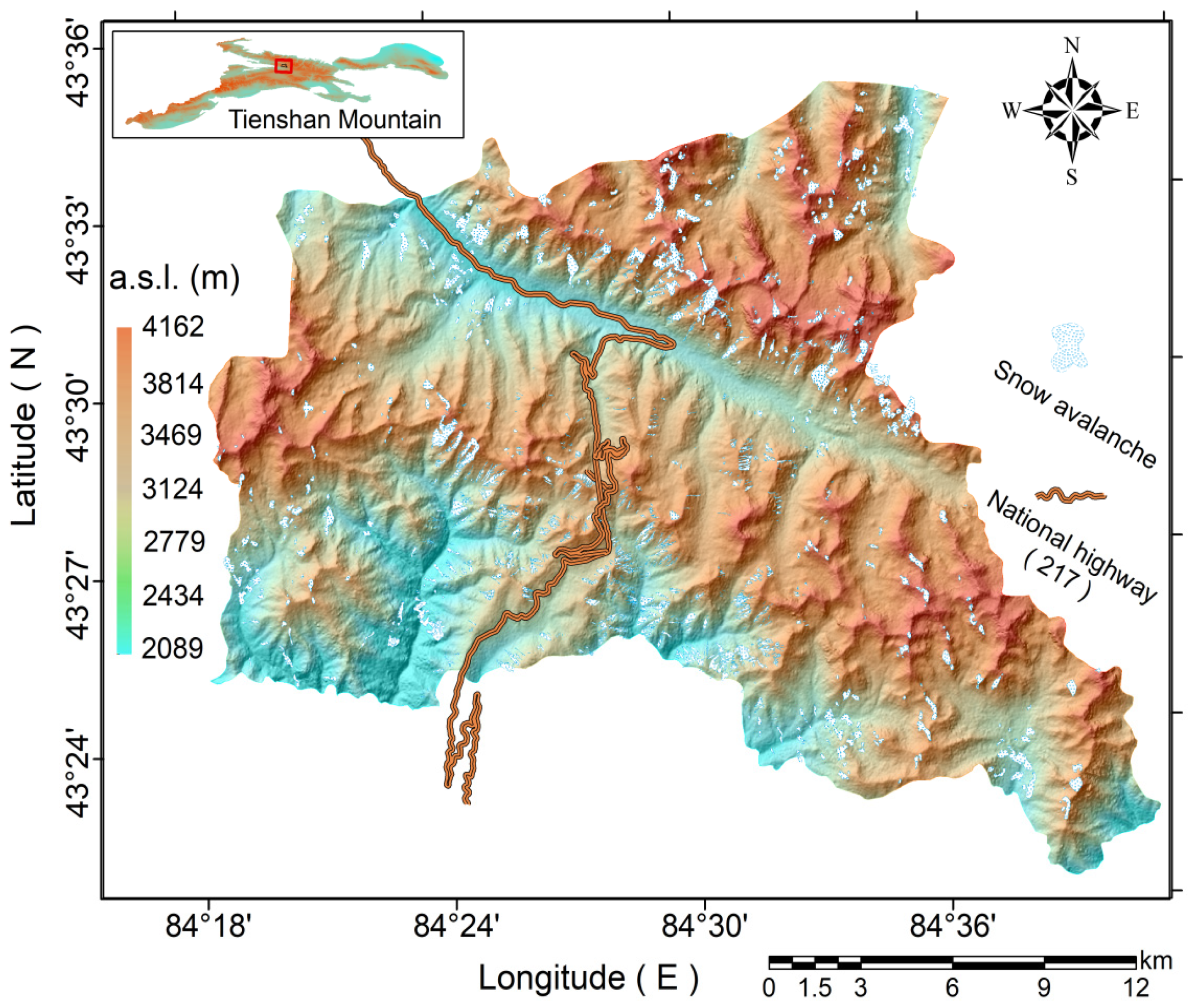
Figure 1. Location of the study area of Taldasha.
Remotesensing 14 01340 g001
Figure 2. Inventory map of avalanches in winter and spring.
Remotesensing 14 01340 g002
Figure 3. Spatial distribution of safe and hazard samples and their seasonal selection differences.
Remotesensing 14 01340 g003
Figure 4. The scene environment of drone photography (a) and the morphological characteristics of avalanche obtained by photography (b).
Remotesensing 14 01340 g004
Figure 5. Work scenarios during field investigation of avalanches.
Remotesensing 14 01340 g005
Figure 6. Avalanche causal factors and their classes.
Remotesensing 14 01340 g006aRemotesensing 14 01340 g006b
Figure 7. Flowchart of the study methodology.
Remotesensing 14 01340 g007
Figure 8. Parameter optimisation results of RF model.
Remotesensing 14 01340 g008
Figure 9. Results of tuning hyper parameters of KNN model.
Remotesensing 14 01340 g009aRemotesensing 14 01340 g009b
Figure 10. Avalanche susceptibility maps and proportion of each hazard level. (a) SVM-Winter, (b) SVM-Spring, (c) SVM-Control group, (d) RF-Winter, (e) RF-Spring, (f) RF-Control group, (g) KNN-Winter, (h) KNN-Spring, (i) KNN-Control group.
Remotesensing 14 01340 g010aRemotesensing 14 01340 g010bRemotesensing 14 01340 g010c
Figure 11. Validation of avalanche susceptibility maps using ROC-AUC: (a) winter, (b) spring and (c) control group.
Remotesensing 14 01340 g011
Table 1. Avalanche hazard assessment methods and their advantages and disadvantages.
Physical Model
AdvantagesCan precisely describe the snow instability process and avalanche dynamics on a single predefined slope.
DisadvantagesHigher reliance on special input data.
Drive data is difficult to obtain.
Limited scale of assessment.
Data-Driven
AdvantagesEasy to implement.
Satisfying visualisation.
DisadvantagesThe evaluation results have certain uncertainty and human subjectivity.
The variable selection process has a certain one-sidedness and fuzziness.
Machine Learning
AdvantagesThe evaluation results are objective and accurate.
The evaluation model can be replicated and extended.
Avalanche hazard can be assessed on a large scale.
DisadvantagesHigh requirements for the quality and quantity of sample data.
Field Observation Assessment
AdvantagesDaily evaluation possible.
DisadvantagesEvaluation results vary and are subjective due to the specialisation of the observers.
Avalanches occur suddenly, resulting in very limited opportunities to prepare and issue alerts.
The scope of the assessment is limited by the natural conditions and the accessibility of the road network.
Table 2. Parameter statistics of collected SV-1 images.
Parameter StatisticsDetails
BandsMultispectralPanchromatic
RedGreenBlueNear Infrared
Spectral range (mm)450–520520–590630–690770–890450–890
Spatial resolution2.0 m50 cm
Revisit period1 d
Ground sampling interval2.0 m
Cloud cover 0.5–2.7%
Table 3. Multicollinearity of the causative factors.
VariablesWinterSpringControl Group
TOLVIFTOLVIFTOLVIF
Elevation0.7511.3320.7131.4030.6751.480
Slope0.9211.0860.9301.0760.7341.447
Aspect0.6611.5120.8531.1720.8571.167
Plane curvature0.4942.0250.6761.4790.6131.631
Profile curvature0.5791.7260.5461.8320.5881.701
TRI0.2474.0480.3862.5910.7361.142
TPI0.3832.6130.3952.5340.4092.445
VRM0.7061.4160.6911.4470.7181.393
TST0.5941.6840.6101.6400.6421.557
RDLS0.2743.6530.5481.8230.6651.504
DTS0.9211.0850.8531.1730.9731.028
TWI0.3512.8510.3123.2010.3173.152
DTR0.7611.3150.5511.8150.8951.118
Solar radiation0.6821.4660.5861.7080.6311.586
Temperature0.6371.5700.1845.4240.5011.937
Wind speed0.4522.2140.2044.9020.1476.808
LUCC0.9591.0420.9471.0560.9131.095
Earthquake hazard distribution0.7441.3450.7131.4030.8171.223
Snow depth0.5181.9320.6731.4860.4072.457
Table 4. Weight of causative factors in Winter, Spring and control group.
WinterSpringControl Group
Causative FactorsWeightCausative FactorsWeightCausative FactorsWeight
RDLS14.18%Snow depth17.33%DTS10.11%
Slope10.72%DTR13.95%DTR10.11%
TST9.24%Temperature7.84%Aspect9.72%
Elevation9.07%Elevation7.02%Slope9.19%
DTS8.76%LUCC6.21%Solar radiance8.82%
TPI7.58%TST5.69%RDLS8.77%
DTR6.85%Slope5.65%Elevation8.47%
Snow depth5.97%TPI5.22%Profile curvature6.97%
Temperature5.74%TWI4.69%TPI5.82%
TRI4.87%RDLS4.61%TWI5.72%
Aspect4.36%VRM4.26%TST4.85%
Solar radiance3.43%Plane curvature4.06%Temperature3.22%
VRM3.38%Wind speed3.98%LUCC2.33%
TWI1.82%Earthquake hazard distribution3.71%TRI2.26%
Wind speed1.77%Profile curvature2.64%Snow depth1.67%
Profile curvature1.03%Aspect2.07%Earthquake hazard distribution1.14%
LUCC0.64%DTS0.59%Wind speed0.69%
Earthquake hazard distribution0.62%Solar radiance0.48%Plane curvature0.19%
Plane curvature0.00%TRI0.00%VRM0.00%
Table 5. The results of Mann-Whitney U test.
VariablesSpringWinterControl Group
U-TestSig. U-TestSig.U-TestSig.
Elevation835,967.50.002449,809.00.0004,835,510.50.000
Slope1,511,322.50.0001,134,259.50.00010,501,820.50.000
Aspect767,895.00.029625,725.50.0305,792,301.50.000
Plane curvature2,640.00.0001,163,187.00.0004,877,144.50.000
Profile curvature1,487,844.00.0001,007,208.00.0006,170,964.50.000
TRI1,549,211.00.0001,163,790.00.00010,470,029.00.000
TPI15,550,256.00.0001,154,167.00.0003,861,983.00.000
VRM0.00.0001,163,790.00.0004,625,425.50.000
TST1,554,297.00.0001,162,073.00.0006,165,772.50.000
RDLS1,506,172.00.000235,121.00.0009,838,493.50.000
DTS903,403.50.000740,014.50.0006,824,133.00.000
TWI1,557,600.00.0001,163,731.00.0004,790,261.00.000
DTR1,036,784.50.000757,006.50.0005,488,534.50.024
Solar radiation977,256.50.000500,320.50.0003,704,101.00.000
Temperature1,169,421.00.0001,127,098.00.0005,724,934.00.000
Wind speed274,446.00.0000.00.0005,133,122.50.001
LUCC899,652.00.000384,258.00.0004,280,161.00.000
Earthquake hazard distribution865,046.00.000633,830.50.0005,453,588.50.016
Snow depth1,281,572.00.0000.00.0005,678,461.00.000
Table 6. Parameters of SVM model.
SeasonsKernelCgNumber of Support VectorsAUC
WinterLinear1/3310.897
Polynomial10.52100.886
RBF10.52470.992
Sigmoid10.57800.846
SpringLinear1/4820.801
Polynomial10.53250.931
RBF10.55640.994
Sigmoid10.57470.928
Control groupLinear1/4860.885
Polynomial10.52910.898
RBF10.58970.995
Sigmoid10.57220.880
Table 7. Indicators to evaluate and compare the results of model performance.
CasesClassifierStatistics
MCCOAFOMPOFDFB
WinterSVM0.8150.8920.1310.0860.892
RF0.9650.9350.1110.0140.652
KNN0.8290.7720.0920.2921.011
SpringSVM0.7600.7570.2700.1880.600
RF0.9050.9850.0030.0630.989
KNN0.7700.7960.2640.1201.218
Control groupSVM0.5520.6880.6550.4601.160
RF0.6870.7300.2190.2970.754
KNN0.4230.6120.3930.3571.601
Table 8. Combined with multi-source heterogeneous variables on the performance of SVM model.
SVM
SeasonsTypes of Factors
Applied One by One
Accuracy Statistics
MCCOAFOMPOFDFB
WinterTopographic0.1090.5420.5620.4501.789
Atmosphere0.3930.5610.5000.3001.421
LUCC0.4890.5780.4720.2721.101
Crustal movement0.5280.6180.4000.2000.774
SpringTopographic0.3060.5010.3620.4700.675
Atmosphere0.3280.5420.2620.3760.626
LUCC1.0110.6730.2060.3520.513
Crustal movement0.5410.7790.1710.2710.648
Table 9. Combined with multi-source heterogeneous variables on the performance of RF model.
RF
SeasonsTypes of Factors
Applied One by One
Accuracy Statistics
MCCOAFOMPOFDFB
WinterTopographic0.59505450.3330.5301.543
Atmosphere0.6790.6320.2580.5001.746
LUCC0.7190.7700.2000.3271.603
Crustal movement0.7990.8480.1630.2580.500
SpringTopographic0.6950.6450.4330.5340.543
Atmosphere0.7050.7050.3340.4950.543
LUCC0.7490.7450.2950.3440.415
Crustal movement0.7810.8410.2640.2780.641
Table 10. Combined with multi-source heterogeneous variables on the performance of KNN model.
KNN
SeasonsTypes of Factors
Applied One by One
Accuracy Statistics
MCCOAFOMPOFDFB
WinterTopographic−0.2190.4100.4240.6521.603
Atmosphere2.0620.4210.3940.4241.553
LUCC1.1450.5500.3360.3361.433
Crustal movement0.2490.6110.3360.2971.285
SpringTopographic1.7190.3520.4240.6521.653
Atmosphere1.6310.4130.3940.4241.453
LUCC1.5100.5210.2890.4581.383
Crustal movement−0.4270.5630.1580.3891.301
Publisher’s Note: MDPI stays neutral with regard to jurisdictional claims in published maps and institutional affiliations.