Abstract
A quantitative understanding of changes in water resources is crucial for local governments to enable timely decision-making to maintain water security. Here, we quantified natural-and human-induced influences on the terrestrial water storage change (TWSC) in Sichuan, Southwest China, with intensive water consumption and climate variability, based on the data from the Gravity Recovery and Climate Experiment (GRACE) and its Follow-on (GRACE-FO) during 2003–2020. We combined the TWSC estimates derived from six GRACE/GRACE-FO solutions based on the uncertainties of each solution estimated from the generalized three-cornered hat method. Metrics of correlation coefficient and contribution rate (CR) were used to evaluate the influence of precipitation, evapotranspiration, runoff, reservoir storage, and total water consumption on TWSC in the entire region and its five economic regions. The results showed that a significant improvement in the fused TWSC was found compared to those derived from a single model. The increase in regional water storage with a rate of 3.83 ± 0.54 mm/a was more influenced by natural factors (CR was 53.17%) compared to human influence (CR was 46.83%). Among the factors, the contribution of reservoir storage was the largest (CR was 42.32%) due to the rapid increase in hydropower stations, followed by precipitation (CR was 35.16%), evapotranspiration (CR was 15.86%), total water consumption (CR was 4.51%), and runoff (CR was 2.15%). Among the five economic regions, natural influence on Chengdu Plain was the highest (CR was 48.21%), while human influence in Northwest Sichuan was the largest (CR was 61.37%). The highest CR of reservoir storage to TWSC was in Northwest Sichuan (61.11%), while the highest CRs of precipitation (35.16%) and evapotranspiration (15.86%) were both in PanXi region. The results suggest that TWSC in Sichuan is affected by natural factors and intense human activities, in particular, the effect of reservoir storage on TWSC is very significant. Our study results can provide beneficial help for the management and assessment of regional water resources.
1. Introduction
Water sources should have sufficient quantity to meet the specific needs of a certain place in a period of time [1]. Freshwater resources on Earth that humans can use are mainly terrestrial water storage (TWS) including surface water storage (such as runoff, lake, wetlands, reservoirs, etc.), soil moisture, groundwater, glacier snow, and vegetation canopy water [2,3]. However, the rapid development of human society has led to a water crisis regionally and even fierce conflicts between countries. Therefore, a comprehensive and accurate investigation into TWS change (TWSC) can help local governments make timely and reasonable measures and decision-makers to maintain the safety of water resources [4].
Sichuan, with an area of 486,000 km2, is located on the upper reaches of the Yangtze River, Southwest China, with parallel valleys and hills in the east, Chengdu Plain in the middle, and Western Sichuan Plateau in the west [5]. By 2020, the permanent population of this region was 83,674,866, with a gross domestic product (GDP) of 4859.88 billion yuan in 2020 [6]. This region has rich water resources, mainly originating from the Yangtze River system. However, the distribution of water resources is uneven in time and space. As a result, water shortages occur regionally and seasonally [7]. Furthermore, Sichuan is a large traditional agricultural province and an important industrial base in China. Therefore, there is a distinct gap between the huge demand for water in industrial/agricultural production, daily human life, and the uneven distribution of water resources in this region. Therefore, it is necessary to conduct reasonable assessments and accurate and timely monitoring of water resources in Sichuan.
Natural factors have a direct influence on regional water resource changes. In particular, the global warming trend has intensified, leading to frequent extreme disasters (flood and drought) around the world. Previous studies [8,9,10] indicate the precipitation (PPT) and evapotranspiration (ET) are the main driving factors of the regional water cycle as well as the important factors leading to regional TWSC. Anyah et al. [11] analyzed the relationship between TWSC in Africa and five climate indices during the period 2003–2012, and the results show that there is a significant correlation between the above natural indices and TWSC. Banerjee et al. [12] studied the TWSC of the world’s 31 basins under global warming, and the results showed that the concurrence of temperature rise and TWSC decline was found in 23 basins. The reason for the decrease in TWSC may be due to the increase in ET and the decrease in snow caused by the increase in temperature.
With the rapid development of society and economy and the process of urbanization, there is a trend of rapid growth in human water demand in many regions of the world. This leads to an imbalance in the supply and demand of regional water resources, which cause regional TWS deficit [13,14,15]. Felfelani et al. [16] used the global land surface hydrological model and satellite-based TWSC to obtain the global TWSC caused by human activities, and found that human activities may have led to a significant reduction in TWSC in the Euphrates, Ganges, Brahmaputra, and Volga River Basins. Feng et al. [17] pointed out that the reason for the continuous reduction in TWSC in North China is due to large-scale groundwater extraction activities. The rate of groundwater depletion in North China was 2.2603 cm/a from 2003 to 2010.
Gravity Recovery and Climate Experiment (GRACE) and its Follow-on (GRACE-FO) missions are jointly developed and managed by the National Aeronautics and Space Administration (NASA) and Deutschen Zentrums für Luft-und Raumfahrt (DLR). Since the implementation of these two missions, their spherical harmonic (SH) coefficient and Mascon solutions have been widely used to detect the spatial and temporal variations of TWS in large-scale regions, especially the regions where the hydrometeorological ground stations are scarce [18]. In addition, GRACE TWSC data have been extensively used in flood and drought evaluations [18,19,20], hydrological component estimation (e.g., runoff, ET, groundwater storage change) [21,22,23], and glacier melting monitoring [24,25]. Some scholars have used GRACE data to study the relationship between regional TWSC and natural factors and human activities [16,26,27]. However, the above studies used a single GRACE solution, which may increase uncertainties of the study due to discrepancies among different GRACE solutions [28]. Although Xie et al. [4] used an integrated use of five GRACE solutions to characterize the TWSC in the Yellow River Basin and investigated the relationships between TWSC and human activities and climatic change, respectively, only the arithmetic average of six GRACE TWSC data was used without considering the uncertainty of different GRACE solutions.
Therefore, in this study, we first used the generalized three-cornered hat method (GTCH) to evaluate the uncertainty of TWSC results from six GRACE solutions. Then, according to the uncertainty results, six GRACE TWSC results were fused by using the least square method based on the uncertainties of each solution. Subsequently, the fused TWSC results were used to characterize the TWSC in Sichuan, Southwest China. Local meteorological data (PPT, ET, runoff) and local human-induced TWS data (reservoir water storage, production water consumption, domestic water consumption, etc.) were further used to investigate the influence of natural and human factors on TWSC in this region. The rest of paper is organized as follows. We briefly introduce the study region, data, and the analysis methods in Section 2, Section 3 and Section 4, respectively. Section 5 presents the analysis results of the contribution of each component of natural- and human-induced TWSC to total TWSC. The discussion and conclusions are provided in Section 6 and Section 7, respectively.
2. Study Area
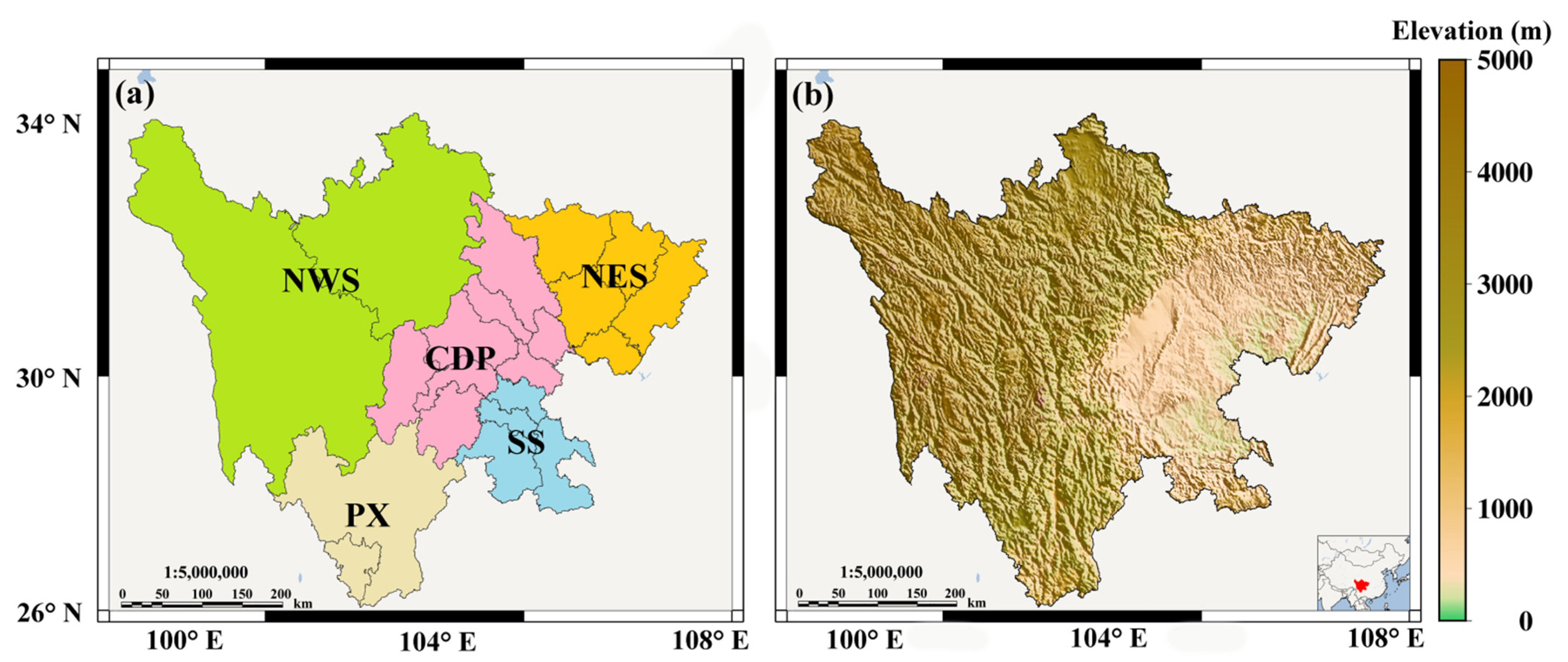
Sichuan is located in Southwestern China, approximately at 26–34°N and 97–108°E (see Figure 1). There is a big difference between the east and the west, and the terrain is high in the west and low in the east, consisting of mountains, hills, plains, basins, and plateaus. This region has three major climates, namely, the humid subtropical climate in the Sichuan Basin, the subtropical semi-humid climate in the mountain of southwest of Sichuan, and the alpine plateau in the northwest of Sichuan [29]. The Yangtze River is the largest river flowing through this region. The main tributaries of Yangtze River in this region include the Ya-lung River, Min River, Tuo River, Jialing River, etc. To better analyze the influence of human activities on TWSC, according to local government standards, we divided Sichuan into five regions, namely Northwest Sichuan (NWS), Chengdu Plain (CDP), Northeast Sichuan (NES), South Sichuan (SS), and PanXi region (PX) (see Figure 1a).
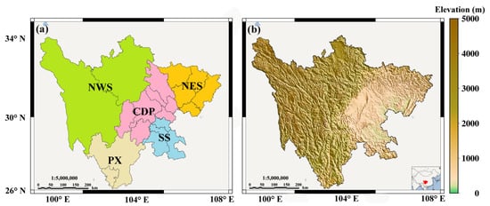
Figure 1.
The economic regions (a) and digital elevation model (b) of Sichuan.
3. Data
3.1. GRACE/GRACE-FO Data
In our study, we used four GRACE/GRACE-FO RL06 SH solutions (truncated to degree and order 60) to extract the monthly 1° × 1° gridded TWSC data in the study region. These four SH solutions were provided by the Center for Space Research at the University of Texas at Austin (CSR), Helmholtz-Center Potsdam-German Research Center for Geosciences (GFZ), Jet Propulsion Laboratory (JPL), and Institute of Geodesy at Graz University of Technology (ITSG), respectively. To improve the accuracy of the TWSC results, we took the following measures. First, to eliminate the influence of geocentric motions on SH solution, the degree-1 coefficients were estimated by using the method of Swenson et al. [30]. Second, due to the low accuracy of the C20 coefficient of the SH solution, the results of satellite laser ranging were used to replace it [31]. Third, we used de-correlation P3M6 and a 300 km Fan filter [18] to weaken the north–south strip and high frequency noises in the TWSC results from SH solution. Finally, GRACE/GRACE-FO signal attenuation was attributed to degree truncation and filtering processing. In our study, the signal attenuation could be recovered by the scale factor method [32]. The monthly 1° × 1° gridded TWSC data could also be obtained from two GRACE/GRACE-FO RL06 Mascon solutions from CSR and JPL. The difference to the SH solution is that the Mascon solution does not need to perform additional processing and the gridded TWSC data can be obtained directly.
In our study, we used these four SH solutions and two Mascon solutions to obtained GRACE/GRACE-FO TWSC gridded data from January 2003 to June 2017 and from June 2018 to December 2020. Since GRACE and GRACE-FO data are essentially the same, we referred to the GRACE and GRACE-FO data as GRACE data. For convenience, these four SH solutions and two Mascon solutions were termed as CSR-SH, GFZ-SH, JPL-SH, ITSG-SH, CSR-M, and JPL-M.
3.2. Reconstructed TWSC Data
Due to an 11-month data gap between GRACE and GRACE-FO mission, we used the dataset of reconstructed TWSC data in China based on PPT (2002–2019) provided by the National Tibetan Plateau Data Center to fill this gap. This dataset was based on the CSR GRACE/GRACE-FO RL06 Mascon solutions, China’s daily gridded PPT real-time analysis system (version 1.0), and CN05.1 temperature data and other datasets by using a PPT reconstruction model, and considering the seasonal items and trend item of CSR RL06 Mascon solutions [33]. The reconstructed TWSC data were calculated according to the following formula [34]:
where is the reconstruction TWSC data; is the monthly PPT data; is the calibration parameter of the long-term trend term; and is the calibration parameter of the seasonal term.
3.3. In Situ PPT Data
In our study, the monthly 0.5° × 0.5° gridded PPT data from January 2003 to December 2020 were provided by the China National Meteorological Science Data Center. The dataset was from the monthly PPT gridded data at national-level stations nationwide from 1961 to the present, which were collected and compiled by the China National Meteorological Information Center.
3.4. GLDAS Model
The Global Land Data Assimilation System (GLDAS) 2.1 model [35] is a hydrological model provided jointly by the Goddard Space Flight Center at NASA and the National Centers for Environmental Prediction at the National Oceanic and Atmospheric. This model contains 4-layer soil moisture, temperature, snow melt, ET, and other hydrological components. The monthly 1° × 1° gridded runoff data from January 2003 to December 2020 were derived from the GLDAS 2.1 Noah models and the monthly GLDAS TWSC from GLDAS 2.1 Noah at a spatial resolution of 1° × 1° are the sum of soil moisture, snow water equivalent, and plant canopy water in our study.
3.5. ET Data
The ET gridded data with a spatial resolution of 0.25° × 0.25° from January 2003 to December 2016 came from the Global Land Evaporation Amsterdam Model (GLEAM) 3.5a [36,37] in our study. The model includes land evaporation, transpiration, bared-soil evaporation, interception loss, open-water evaporation, and sublimation. Additionally, GLEAM provides surface and root-zone soil moisture, potential evaporation, and evaporative stress conditions.
3.6. Human-Induced TWSC Data
The human-induced TWSC data were derived from the Sichuan Province Water Resources Bulletins that were published by the Sichuan Provincial Water Resources Department for the period of 2003–2020 [38]. The bulletin provided the annual values of precipitation, runoff depth, groundwater storage, reservoir storage, total water supply, total water consumption, agricultural water consumption, industrial water consumption, domestic water consumption, and ecological water consumption in Sichuan Province and its administrative regions.
4. Methods
4.1. Fusing Different Datasets
Due to the discrepancies between different datasets, if a single dataset is used for data analysis, unreliable results may be obtained. Therefore, to eliminate these discrepancies and improve the reliability of the analysis results, we first used the GTCH method to estimate the relative uncertainties of six GRACE TWSC results. The advantage of the GTCH method is that it does not require prior information [39]. Then, the six GRACE TWSC results were fused according to their uncertainties by using the least square method. Considering that the spatial resolutions of different data are inconsistent, we used the spatial re-sampling method to unify the spatial resolution between the different data.
4.1.1. The GTCH Method
Suppose there are several different observation series, and these time series can be expressed as:
where is the real signal; is the noise of the observation series (0 means white noise); and is the number of observation series. Because the real signal cannot be obtained, the noise of the observation series cannot be known. To solve the problem of noise estimation under the condition of no prior information, we chose any observation series as the reference series, and the choice of the reference series does not influence the final results [40]. The relationship between the reference series and the remaining observation series can be expressed as:
where is the reference observation series and is the noise of the reference observation series. is the difference between the remaining observation series and the reference observation series. In this study, we selected the TWSC series from JPL-M as the reference series. The different observation series can be combined into the following matrix.
where is the number of observations in the series. The corresponding covariance matrix S between N − 1 different observation series is
where is the covariance operator. is the variance and covariance , that is, the variance or covariance of different series between the remaining TWSC series from five GRACE solutions and the reference series.
The unknown noise covariance matrix R can be expressed as:
where .
The relationship of R with S is [39]:
where the matrix J is:
From Equation (7), the following relationship can be obtained:
Both R and S are real symmetric matrices by definition. There are unknown parameters to be found for R, but there are only equations for S. Therefore, Equation (6) is underdetermined. As a result, the remaining N free parameters need a reasonable way to obtain a unique solution [41].
To ensure the positive definiteness of matrix R, Galindo and Palacio [42] proposed an important constraint on the solution space for free parameters based on the Kuhn–Tucker theorem. The expression is as follows:
where , which is introduced for a better numerical solution. is given by [43]:
Equation (10) constrains the free parameters in the solution domain, but it is not enough to determine the unique solution of the free parameters [44]. Therefore, it is necessary to provide the optimal selection criteria to determine the unique parameter solution. Tavella and Premoli [40] proposed that the minimum “global correlation” of all observation series and the positive definiteness of R were used as the constraints to determine the free parameters. Therefore, the following objective function was defined and minimized to determine the free parameters [42]:
To make the initial value within the constraints, the initial value of the iterative calculation was set to [40]
Under the constraints of Equation (10), the objective function (Equation (12)) was minimized to estimate a set of free parameter solutions, that is, the variance of the uncertainties of different observation series. Other unknown elements in R can be determined by Equation (9).
4.1.2. Data Fusion
According to the relative covariance of different datasets obtained by using the GTCH method, we fused the different datasets by taking a weighted average of them [45].
where and are the TWSC results from the individual GRACE solutions and its corresponding weight, respectively. The weights were determined based on the estimated variances.
where is the variance of the th TWSC time series estimates by the GTCH method. The above process was performed grid by grid until we fused the TWSC results from the six GRACE solutions on all the grid nodes.
4.2. Pearson Correlation Analysis
In this study, we used the Pearson correlation analysis to evaluate the relationship between two sets of data. In statistics, the covariance of the two sets of data is generally divided by the standard deviation of the corresponding data series to obtain the Pearson correlation coefficient [4]. For two sets of time series and , the Pearson correlation coefficient can be estimated by the following expression:
where is the number of observations in the time series and ; and and are the average values of the time series and during the study period. The value range of is between −1 and 1.
4.3. Time Series Analysis
The time series of observations contain the long-term trend change term, acceleration term, seasonal change term (annual change and semi-annual change), and residual term. The corresponding terms can be extracted from the linear fitting model. The decomposition is expressed as follows [39]:
where is the time series of TWSC; is the time; is the midpoint of the entire research period; is the residual term; and , , , , , , and are the unknown parameters; is the constant term; is the long-term trend change, is the acceleration; and are annual terms; and and are semi-annual terms. The annual amplitude and annual phase are expressed as follows:
4.4. Natural-Induced and Human-Induced TWSC
To analyze the influence of natural and human factors on regional TWSC, we need to obtain the natural-induced and human-induced TWSC. The natural-induced TWSC (TWSCc) can be obtained from the water balance equation. The water balance equation can be expressed as [8]:
where is the natural-induced TWSC; and and are the total water input and output to the region during the study period, respectively.
If the terrestrial is taken as the research object, the water balance equation can be rewritten as:
where is PPT; is ET; and is runoff.
The expression of human-induced TWSC is as follows:
where TWSCh is the human-induced TWSC; TWSC is GRACE TWSC; and TWSCc is the natural-induced TWSC.
4.5. Contribution Rate
To better understand the contribution of different hydrological components to TWSC, we introduced the contribution rate (CR) to evaluate the role of different hydrological components in modulating TWSC in this region [46].
where is the mean absolute deviation of a TWSC component in the study region. is the number of TWSC components. The expression of is as follows:
where is the element in a TWSC component time series; is the number of elements in the TWSC time series; and is the average value of time series of the TWSC component.
5. Results
5.1. GRACE Solution Fusion
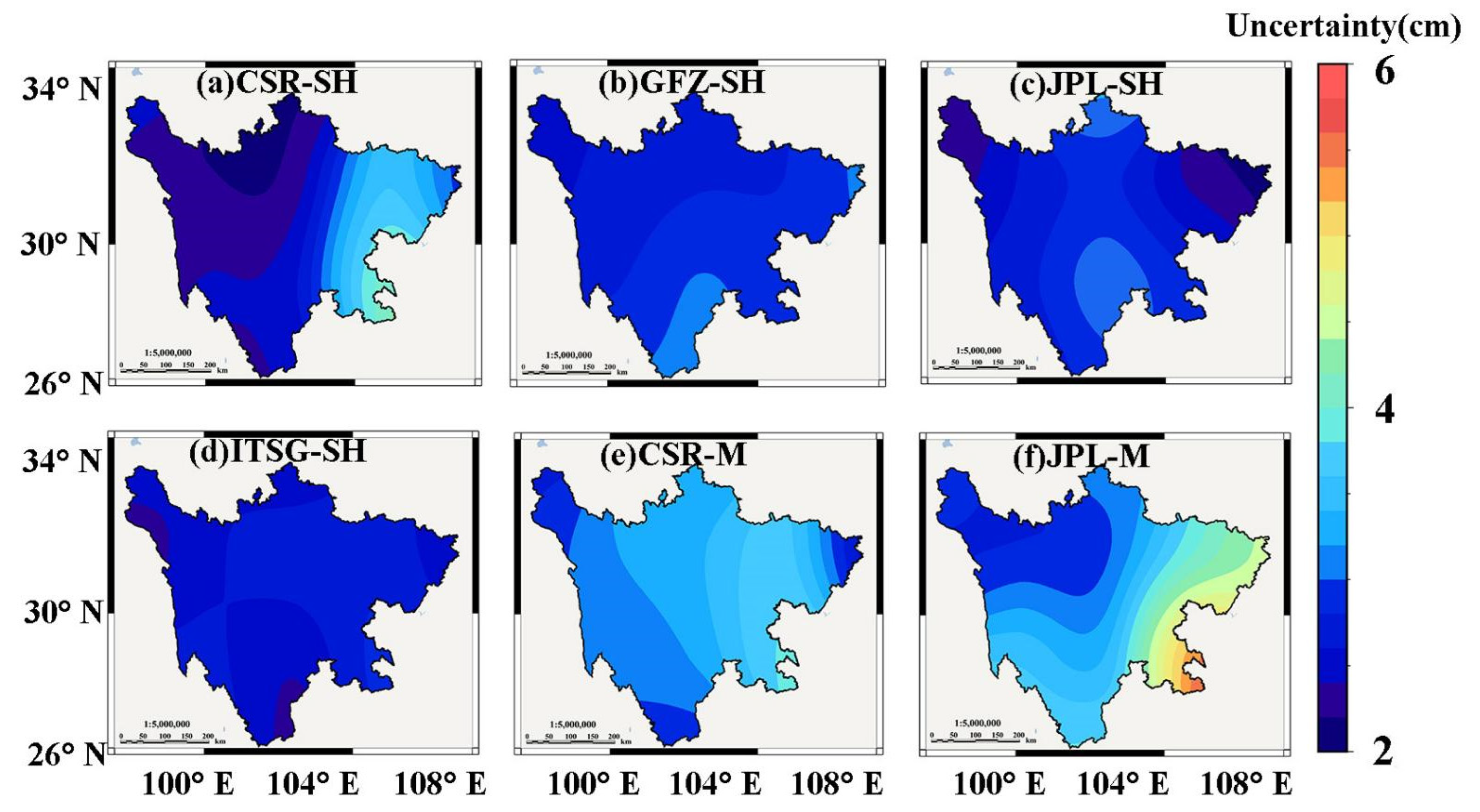
Figure 2 shows the spatial distribution of uncertainties of the six GRACE TWSC results estimated with the use of the GTCH method for Sichuan. Among the six GRACE TWSC results, the uncertainties of the TWSC results from the two Mascon solutions (CSR-M and JPL-M) were larger than the ones from the four SH solutions (CSR-SH, GFZ-SH, JPL-SH, and ITSG-SH). TWSC results from the four GRACE SH solutions and CSR-M typically exhibited uncertainties lower than 3.8 cm for the research region, while TWSC results from JPL-M showed uncertainties greater than 4.4 cm in Southeast Sichuan. In particular, the uncertainties of the TWSC results from JPL-M were higher than 5.4 cm in the part of Southeast Sichuan.

Figure 2.
The spatial distribution of uncertainties of the TWSC results derived from the CSR-SH (a), GFZ-SH (b), JPL-SH (c), ITSG-SH (d), CSR-M (e), and JPL-M (f) solutions estimated by the GTCH method.
We sorted the uncertainties from all grid points in the research region in ascending order and took the median value to evaluate the uncertainty of six GRACE solutions in the whole research region. The results are presented in Table 1. These six GRACE solutions were sorted in ascending order of the uncertainty of the TWSC results, and their arrangement was ITSG-SH (2.34 cm), CSR-SH (2.43 cm), JPL-SH (2.50 cm), GFZ-SH (2.83 cm), JPL-M (3.16 cm), and CSR-M (3.20 cm). This suggests that there are some differences in the uncertainties of TWSC results from different GRACE solutions.

Table 1.
Uncertainties of the TWSC results derived from the six GRACE solutions and fused results estimated by the GTCH method.
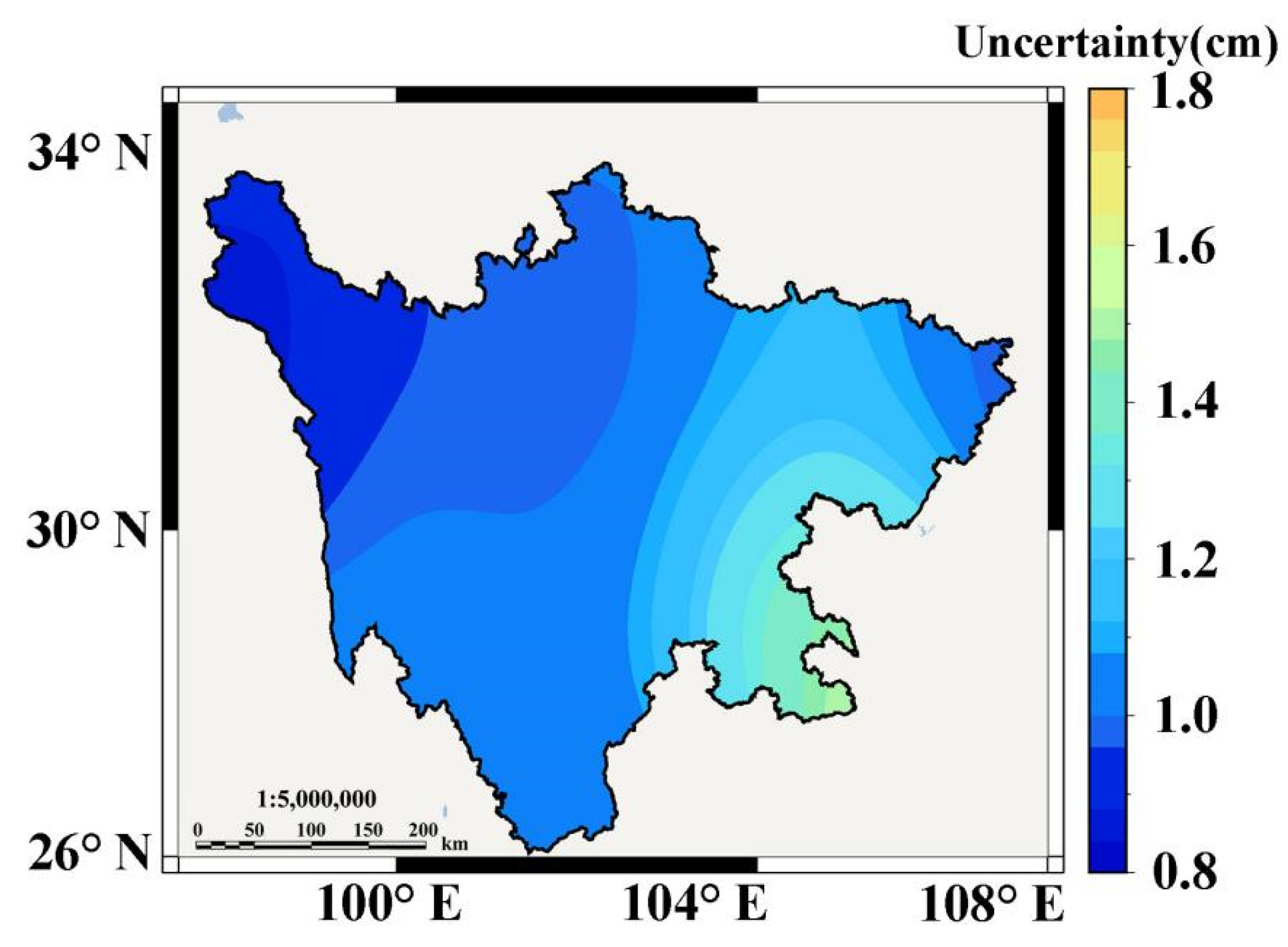
To improve the reliability of the TWSC results, we fused the TWSC results from six GRACE solutions by the least square method based on the variances estimated by the GTCH method. To evaluate the fused effect, we re-calculated the uncertainties of fused results (Figure 3 and Table 1). The uncertainties of fused results were lower than 1.6 cm. The regions with high certainties were mainly concentrated in Southeast Sichuan. The uncertainties of fused results ranged from 1.4~1.6 cm. From Table 1, the medium of uncertainties of fused TWSC results (0.99 mm) was much smaller than those from the six GRACE solutions. This explains that the accuracy of the fused results was better than those of the six single solutions and the fused results obtained by the method in this paper effectively improved the accuracy of the TWSC results in Sichuan.

Figure 3.
The spatial distribution of uncertainties of the TWSC results derived from the fused results.
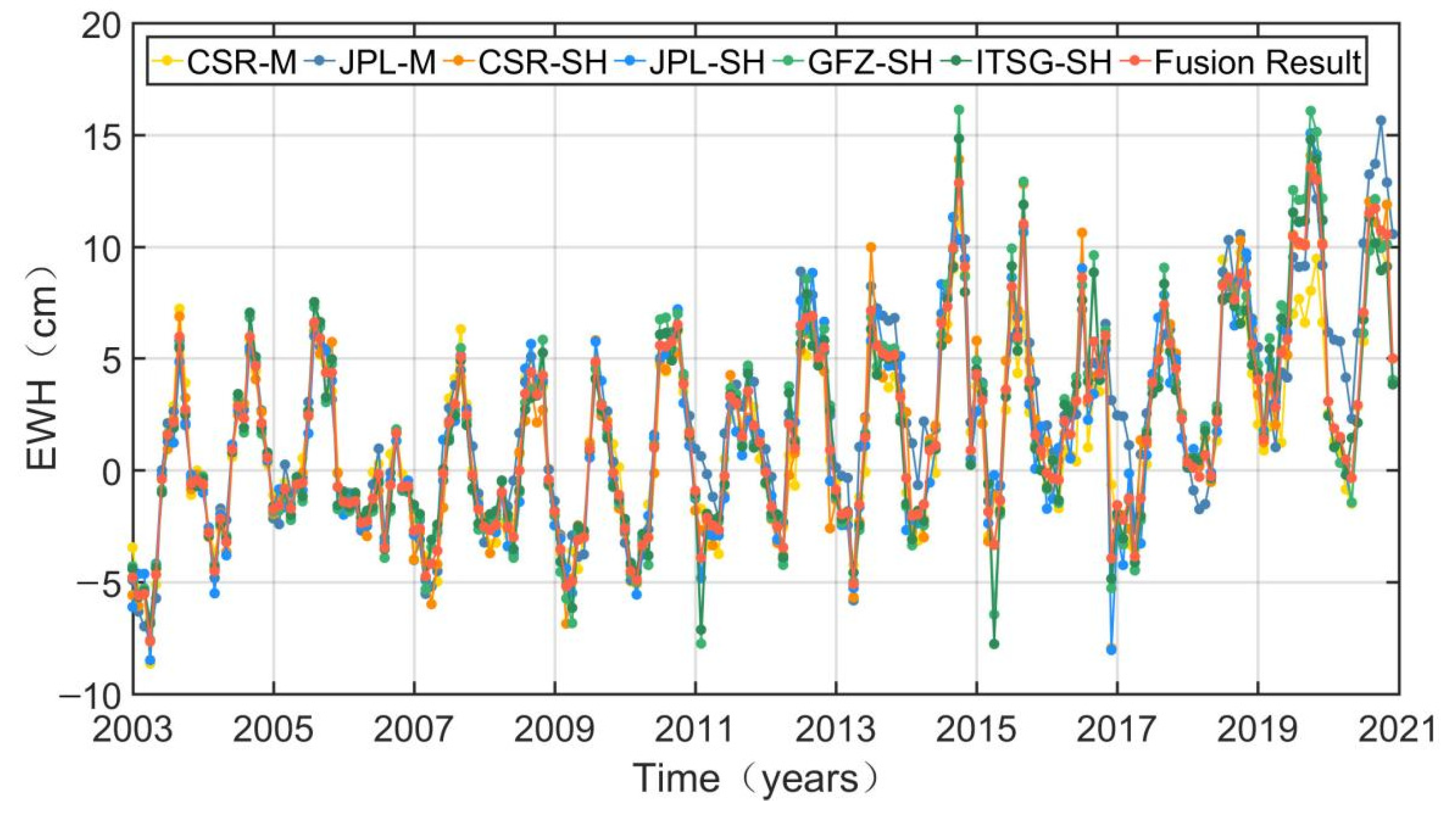
To further evaluate the fused effect, we compared the time series of TWSC from six GRACE solutions and fused results between 2003 and 2020 (Figure 4). From Figure 4, seven TWSC results had a similar change trend. Among the six GRACE TWSC results, the magnitudes of TWSC results from the four SH solutions were larger than those from the two Mascon solutions. We also found that the magnitude of fused TWSC results was close to those from SH solutions. This is because the TWSC results from SH solutions had smaller uncertainties and thus had larger weights in data fusing than the two Mascon solutions. We calculated the correlation coefficients between the fused TWSC results and TWSC results from the six GRACE solutions (Table 2). From Table 2, the correlation of the fused TWSC results with TWSC results from GFZ-SH (0.9822) was the highest, followed by ITSG-SH (0.9818), CSR-SH (0.9811), CSR-M (0.9800), and JPL-SH (0.9674), the smallest correlation coefficient with the fused TWSC results was JPL-M (0.9504). The correlation coefficients between the fused TWSC results and TWSC results from the six GRACE solutions were greater than 0.95.
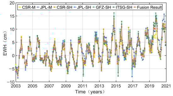
Figure 4.
The time-series of TWSC derived from the six GRACE solutions and fused results.
Table 2.
The correlation coefficients between the fused results and TWSC results from the six GRACE solutions.
We also calculated the long-term trend change, acceleration, annual amplitude, and annual phase of TWSC from the fused results and six GRACE solutions in Sichuan (Table 3). From Table 3, we found that the long-term trend change result of fused TWSC results was close to those from the SH solutions, the acceleration of seven TWSC results were very close, and the annual amplitude and phase of seven TWSC results showed little difference. Therefore, such high correlations and the time series analysis results suggest that the fused TWSC results had high consistency with the TWSC results from the six GRACE solutions.
Table 3.
The long-term change trend, acceleration, annual amplitude, and annual phase of TWSC from the fused results and the six GRACE solutions in Sichuan.
5.2. Spatial and Temporal Distribution of TWSC
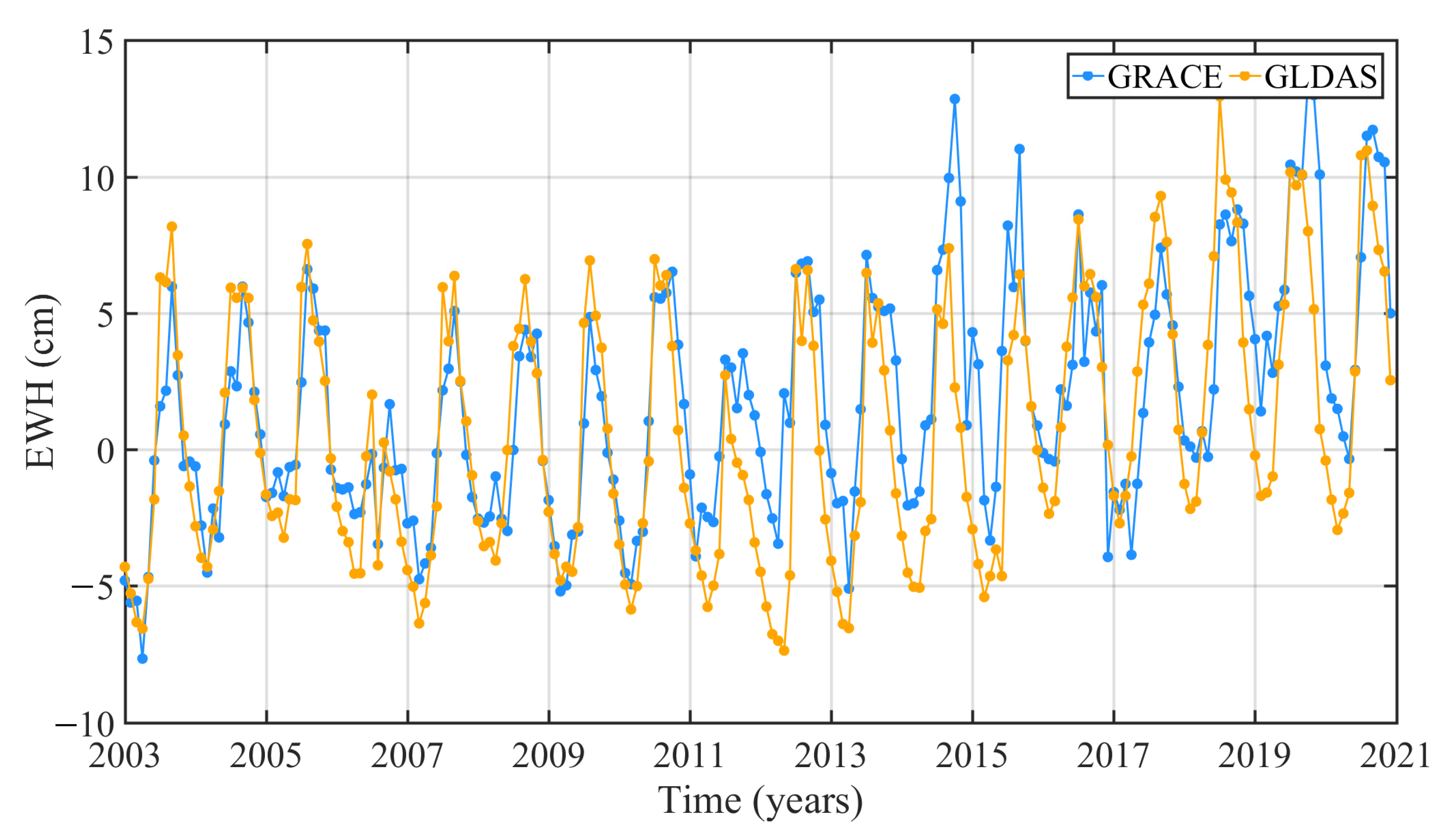
Figure 5 shows that the time series of the fused TWSC results and GLDAS TWSC results. It shows that these two TWSC time series had significant seasonal variation and ta similar change trend. The long-term change trend of TWSC in Sichuan can be divided into two different periods. One is from 2003 to 2011, and there was no significant change in TWSC. The other was from 2011 to 2020, where TWSC showed an increasing trend. Therefore, we calculated the long-term trend change of the fused TWSC results and GLDAS TWSC for three different periods (2003–2020, 2003–2011, and 2011–2020), respectively. The results are shown in Table 4. From Table 4, the long-term change trend of fused TWSC results and GLDAS TWSC during 2003–2020 were 3.83 ± 0.54 mm/a and 2.43 ± 0.52 mm/a, respectively. This suggests that TWSC in Sichuan showed a growth trend in this period. However, TWSC did not grow all the time. Between 2003 and 2011, there was no significant change in the long-term trend change of TWSC in Sichuan. In this period, the long-term trend change of the TWSC results were 0.71 ± 1.62 mm/a (fused results) and −0.34 ± 0.96 mm/a (GLDAS), respectively. Although the two results showed opposite change trends, their values were close to 1 mm/a. Therefore, the difference between the two results was negligible. The increase in TWSC in Sichuan was mainly concentrated in 2011–2020. The long-term trend change of two TWSC results in this period are 5.45 ± 1.43 mm/a and 7.92 ± 1.19 mm/a, respectively. This may be attributed to the development of large-scale hydropower stations [47]. We also plotted the map on the spatial distribution of long-term trend change and the acceleration of fused TWSC results in Sichuan during 2003–2020 (Figure 6).
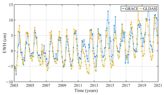
Figure 5.
The time-series of TWSC from the fused results and GLDAS 2.1 model.
Table 4.
The long-term change trend of TWSC in Sichuan Province (unit: mm/a).
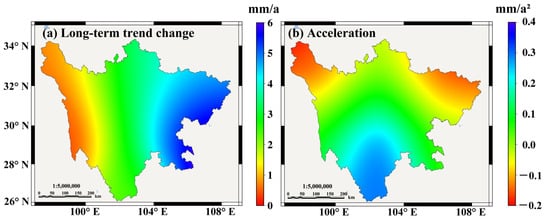
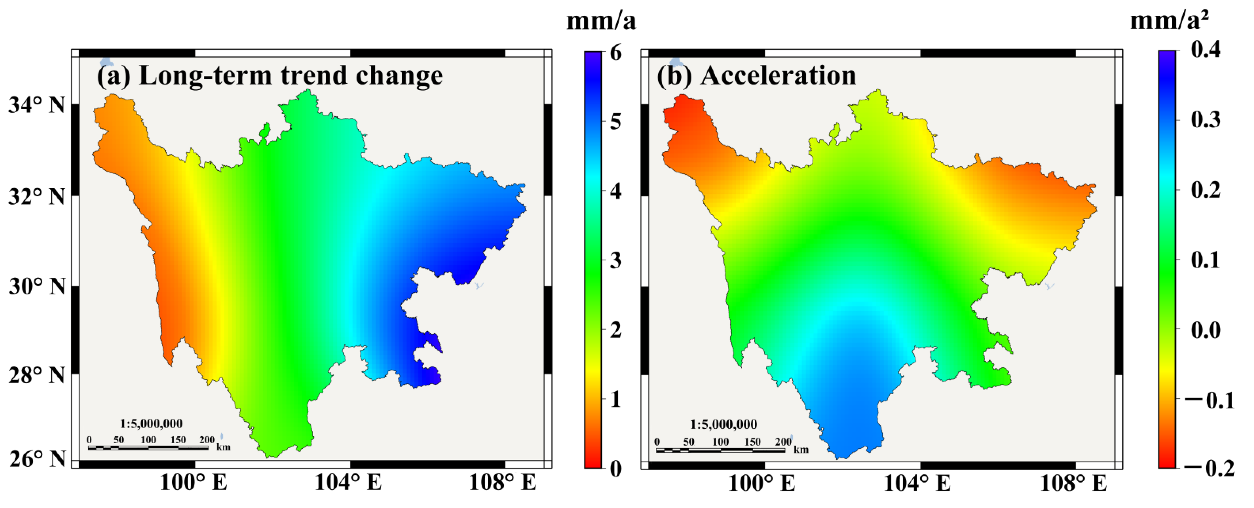
Figure 6.
The spatial distribution of long-term trend changes (a) and acceleration (b) of TWSC in Sichuan Province.
From Figure 6a, TWSC mainly showed an increasing trend in Sichuan. The region with the largest growth was the eastern part of Sichuan (4~6 mm/a), followed by the central and western parts of Sichuan (1.5~4 mm/a and 0~1.5 mm/a). Combining Figure 6a,b, it showed that there was a significant slowing growth trend in the northwestern and northeastern parts of Sichuan, while a significant accelerating increasing trend appeared in the southern part of Sichuan. The reason for the slowing growth trend of TWSC in the northwestern parts of Sichuan may be due to the melting of mountain glaciers caused by global warming [47].
5.3. The Correlation Analysis between TWSC and Natural Variability
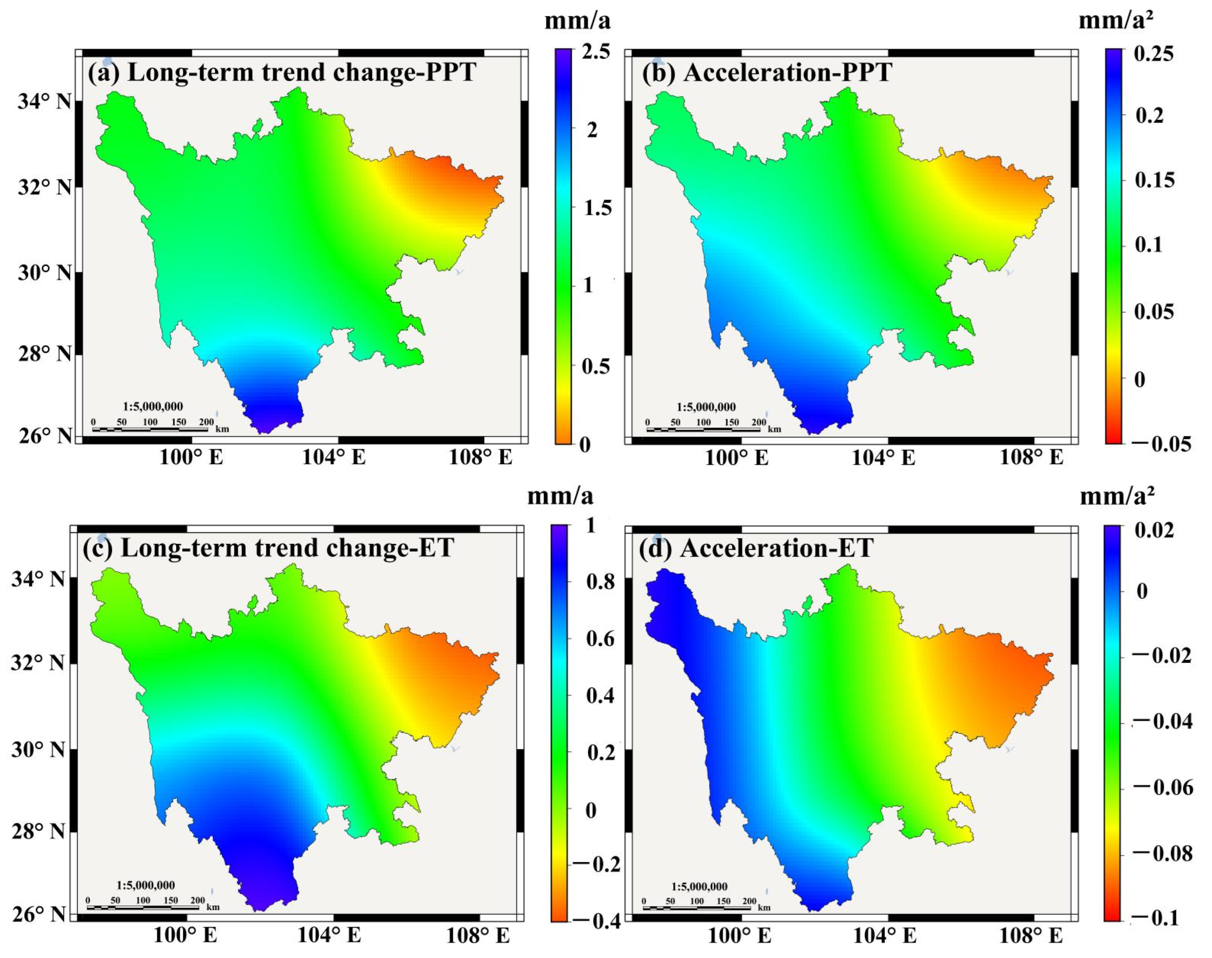
PPT and ET are the two most important meteorological variables and can reflect the influence of climate change [48,49]. Therefore, we analyzed the spatial distribution of long-term trend change and the acceleration of PPT and ET in Sichuan (Figure 7). From Figure 7a, PPT showed an increasing trend in the research region, which is consistent with the variation of TWS (Figure 6a). Among them, the region with the most significant growth trend was the southern part of Sichuan (long-term trend change ranged from 1.5~2.5 mm/a), while the increasing trend was not significant in the northeastern part of Sichuan, which ranged from 0~0.5 mm/a. Except for the northeastern part of Sichuan, the acceleration changes in the other study regions were all positive (Figure 7b). The acceleration in the southern part was the largest, which ranged from 0.1~0.25 mm/a2.
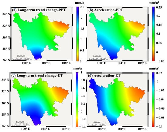
Figure 7.
The spatial distribution of long-term trend changes and the acceleration of PPT and ET in Sichuan. (a) long-term trend change of PPT; (b) acceleration of PPT; (c) long-term trend change of ET; (d) acceleration of ET.
Figure 6 shows that there were the significant increasing trends of ET in most regions of Sichuan, except for the northeast of Sichuan. In particular, the increase in ET in the southern part of Sichuan ranged from 0.6~1 mm/a. In terms of acceleration (Figure 7d), the change trend of TWSC in most regions of Sichuan generally showed a slowing trend and those in the western and southern part of Sichuan showed an accelerating trend. When compared in Figure 7a,c, although PPT and ET showed increasing trends in most regions of Sichuan, the growth rate of PPT was greater than that of ET. Therefore, it led to an increase in TWSC (Figure 6a) without considering other factors. Comparing Figure 6 and Figure 7, the change trend of TWSC in the southern part of Sichuan more clearly indicated that the increase in TWSC was mainly caused by PPT, and the slowdown in the increasing trend of TWSC in northeastern Sichuan was also attributed to the slowdown in the growth trend of PPT.
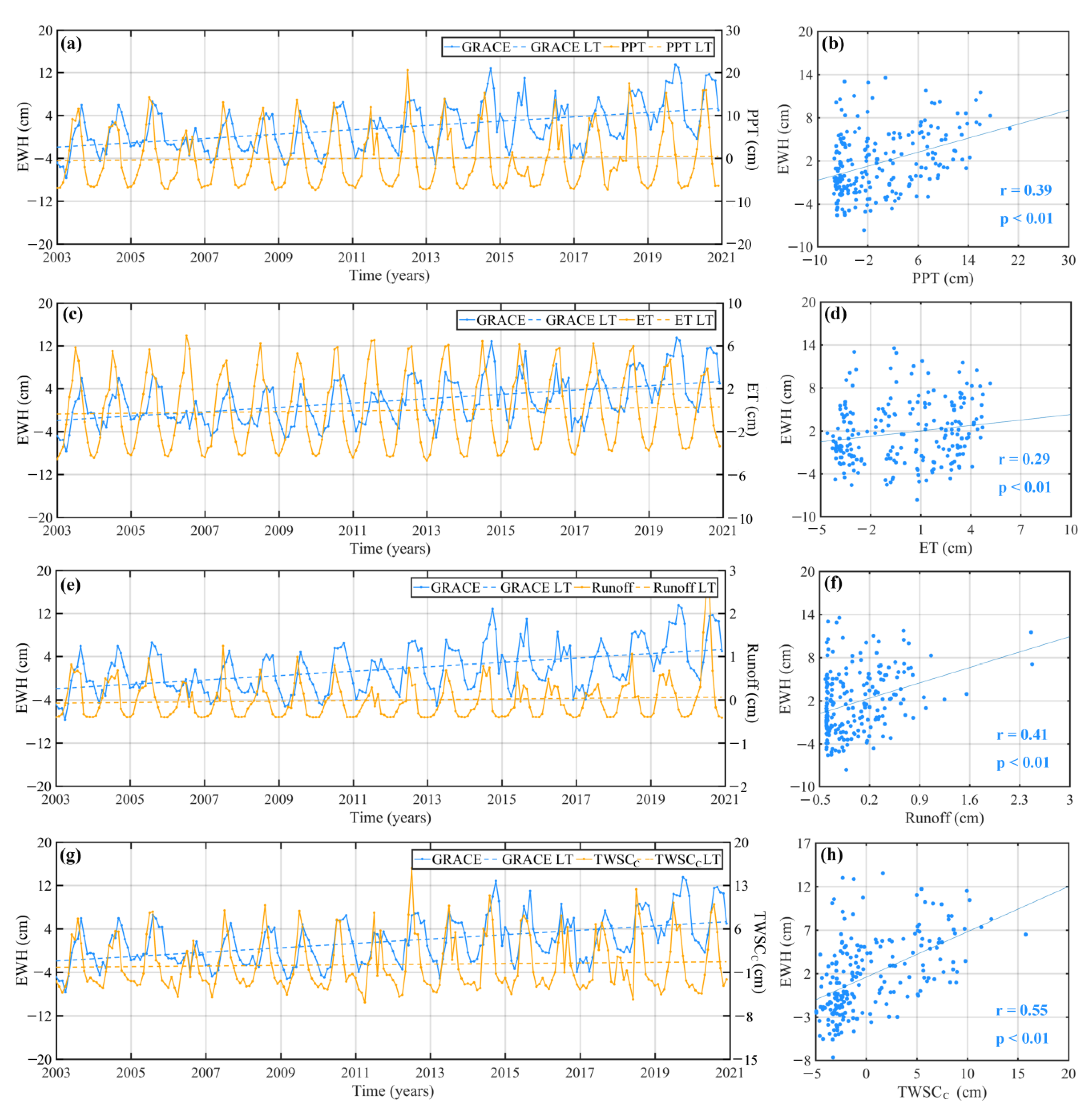
To describe the influence of natural factors on TWSC in the research region, we compared the time series of monthly TWSC with PPT, ET, runoff, and TWSCc in the study period and calculated the correlation coefficients between TWSC and PPT, ET, runoff, and TWSCc (Figure 8). As the main input source of TWSC, PPT has always been regarded as one of the most important factors affecting regional TWSC. Figure 8 shows that PPT, ET, and runoff variations in the study period were about −10~20 cm, −6~6 cm, and −0.5~3 cm, respectively. This shows that the amplitude of the time series of PPT was greater than that of ET and runoff. TWSC, PPT, ET, and runoff had the significant seasonality, but there was no significant correlation between TWSC and PPT, ET, and runoff. Comparing Figure 8b,d,f, the natural factor with the strongest correlation with TWSC was runoff (0.41), followed by PPT (0.39) and ET (0.29). According to Equation (20), we calculated the time series of TWSCc data. Figure 8h shows that TWSC had a strong correlation with TWSCc. Table 5 shows the long-term trend change, acceleration, annual amplitude, and annual phase of TWSC, PPT, ET, runoff, and TWSCc. From Table 5, PPT had a significant increasing trend (1.42 ± 0.69 mm/a), but the change trend of ET and runoff was not as significant (0.32 ± 0.17 mm/a and 0.07 ± 0.07 mm/a). The increasing trend of TWSCc (0.37 ± 0.53 mm/a) was not significant. This suggests that the main reason for the growth of TWSC (3.83 ± 0.54 mm/a) was not from natural factors.
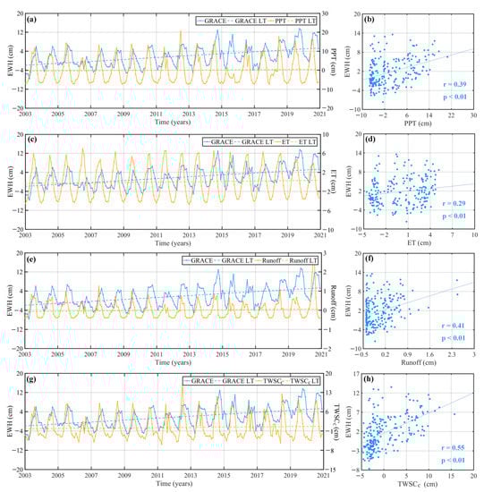
Figure 8.
The relationships between monthly TWSC and ET, PPT, runoff, and TWSCc, respectively, in Sichuan during 2003~2020. (a,c,e,g) show the time series and long-term trend changes of PPT, ET, runoff and TWSCc, respectively; (b,d,f,h) show the correlation coefficients between TWSC and PPT, ET, runoff, TWSCc, respectively.
Table 5.
The long-term change trend, acceleration, annual amplitude, and annual phase of TWSC and natural factors in Sichuan.
To study the correlation between the nature factors and TWSC in the different regions of Sichuan, we also calculated the correlation coefficients between TWSC and the above natural factors in five economic regions of Sichuan (Table 6). The results in Table 4 all passed the significant test of p < 0.01. In the five regions, the three natural factors and TWSCc had no significant correlation with TWSC. We found that there were differences in the correlation between natural factors and TWSC in the different region. Among the five regions, the strongest correlation was between TWSC and TWSCc in CDP (0.41) because the correlation coefficient between TWSC and runoff was the largest in CDP (0.48) and the correlation between TWSC and PPT in CDP (0.41) was second only to the one in NWS (0.42). This may be related to the abundant rainfall and dense river network in CDP [5]. In PX, the correlation between TWSC and ET was the strongest (0.45), which is due to the abundant sunlight in the region [5].
Table 6.
The correlation coefficients between the different factors from climate change and TWSC in Sichuan and its five regions.
5.4. The Correlation Analysis between TWSC and Human Variability
Except for the natural factors, human activities also had an important influence on regional TWSC [50,51]. The influence of human activities on regional TWSC was mainly through the two aspects of total water consumption for human activities and reservoir storage. The total water consumption includes production, domestic and ecological water consumption, and production water consumption contains industrial and agricultural water consumption.
We analyzed the water storage changes caused by human activities in Sichuan from 2003 to 2020 (Figure 9). From Figure 9a, we found that total water consumption was greater than reservoir storage during 2003–2011. After 2011, the reservoir storage increased dramatically and exceeded the total water consumption. This increasing trend continued until 2015. In the five-year period, the reservoir storage in Sichuan increased from 16.628 billion m3 to 53.881 billion m3, an increase of more than three times. From 2015 to 2020, the growth rate of reservoir storage basically flattened. The total water consumption had no significant change during the study period.
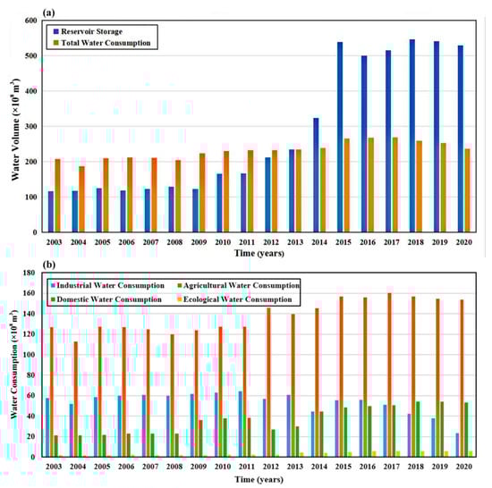
Figure 9.
Statistics of water storage related to human activities in Sichuan from 2003 to 2020. (a) annual change of reservoir storage and total water consumption; (b) annual change of industrial, agricultural, domestic and ecological water consumption.
Figure 9b presents the annual variation of industrial, agricultural, domestic and ecological water consumption in the study period. It shows that agricultural water consumption was the largest and had a significant growth trend. This is because Sichuan is one of the most important agricultural production bases in China [6]. Industrial water consumption maintained a steady state during 2003~2013. From 2014, industrial water consumption dropped from 6.067 billion m3 to 4.473 billion m3. Subsequently, it began to increase year by year until 2016 (from 4.473 billion m3 to 5.583 billion m3). From 2016, it started to decrease continuously and reached the lowest point (2.352 billion m3) in 2020. We found that the annual average of industrial water consumption from 2014 to 2020 (4.446 billion m3) was significantly smaller than that from 2003 to 2013 (5.964 billion m3). This was closely related to the implementation of a water-saving production strategy in Sichuan [52]. Domestic water consumption remained relatively stable from 2003 to 2008. Since 2009, there has been a significant change in the domestic water consumption. Domestic water consumption from 2009 to 2020 (the average was 4.378 billion m3) was significantly higher than the one from 2003 to 2008 (the average is 2.220 billion m3). This is related to the rapid development of the national economy in Sichuan and the continuous growth of urban population [6]. Before 2017, industrial water consumption was always larger than domestic water consumption, but domestic water consumption exceeded industrial water use after 2017, which is the result of the continuous promotion of water-saving production and urbanization. Because ecological water consumption was relatively small, it can be ignored.
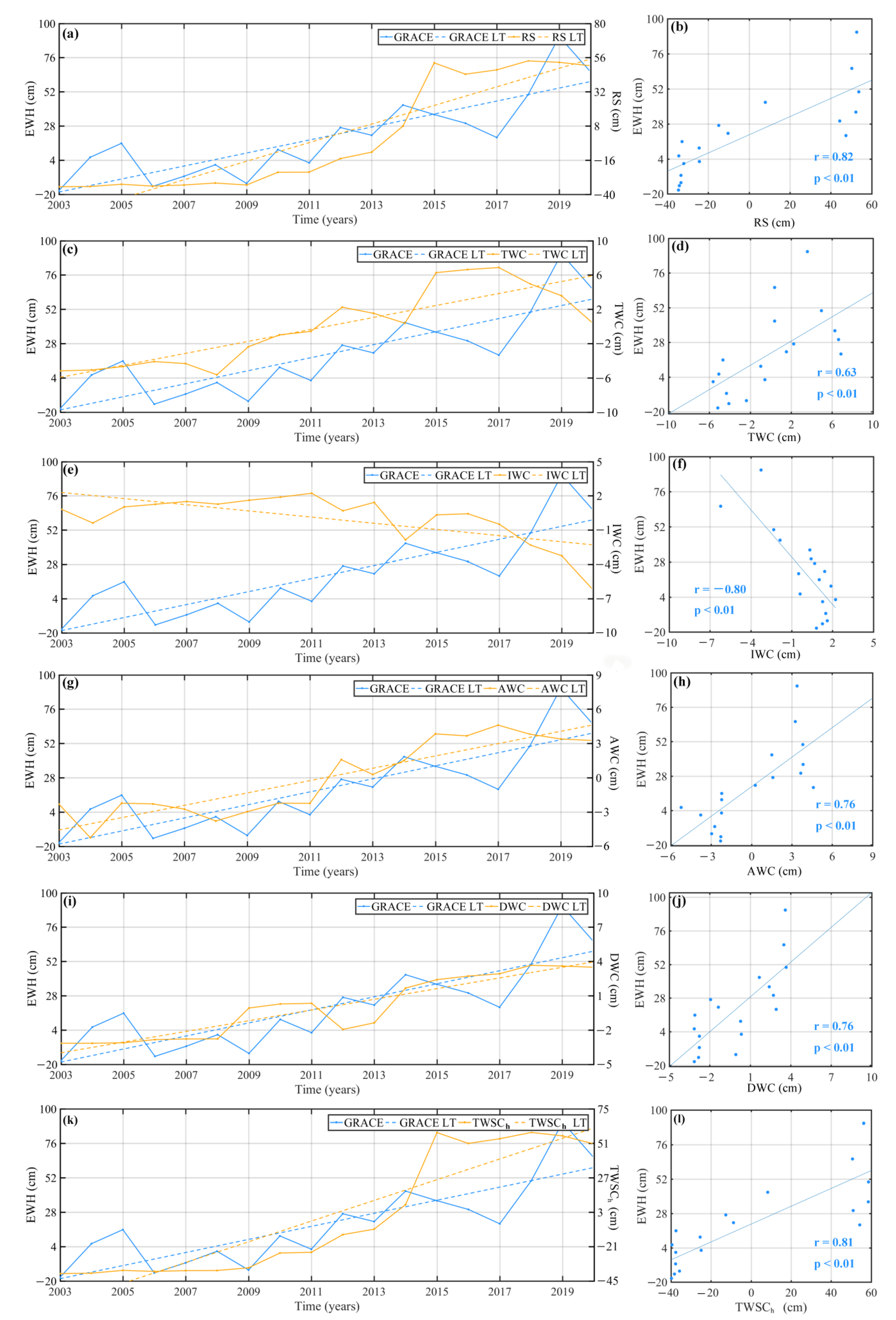
We compared the annual variation of TWSC with reservoir water storage, total water consumption, industrial water consumption, agricultural water consumption, domestic water consumption, and TWSCh and calculated the correlation coefficients between TWSC and six human factors in Sichuan during 2003~2020 (Figure 10). From Figure 10a,b, reservoir water storage was strongly correlated with TWSC in Sichuan (0.82). Previous studies [53,54,55] indicated that when large-scale reservoirs are operated, TWSC in the region where the reservoir is located and the surrounding regions has a significant influence. Since 1996, China has implemented the West–East Power Transmission Strategy. In Sichuan, a large number of hydropower stations have been built on the main streams of the Jinsha, Yalong and Min Rivers. Particularly, a series of large-scale hydropower stations represented by Xiangjiaba and Xiluodu have been put into operation one after another since 2014. The installed capacity of hydropower stations under construction and already under construction has increased from 16.3 million kW in 2003 to 101.74 million kW in 2017, an increase of more than six times [56]. Sichuan has become the largest hydropower base in China [56,57]. The large-scale water storage, flood discharge, and power generation activities cause drastic changes in the reservoir storage, which inevitably have a significant influence on TWSC in Sichuan [58].
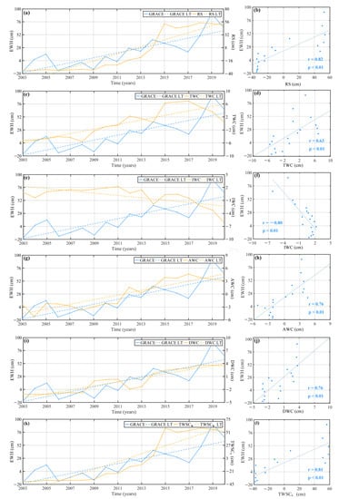
Figure 10.
The relationships between monthly TWSC and RS, TWC, IWC AWC, DWC and TWSCh, respectively, in Sichuan. RS: reservoir storage; TWC: total water consumption; IWC: industrial water consumption; AWC: agriculture water consumption; DWC: domestic water consumption. (a,c,e,g,i,k) show the time series and long-term trend changes of RS, TWC, IWC AWC, DWC and TWSCh, respectively; (b,d,f,h,j,l) show the correlation coefficient between TWSC and RS, TWC, IWC AWC, DWC, TWSCh, respectively.
In addition to reservoir storage, human-related water consumption also had a significant influence on TWSC because Sichuan is one of the most populous provinces in China. As of 1 November 2020, the permanent population of Sichuan was 83.67 million. Sichuan is a traditional agricultural province, and is also an industrial base with the most complete industrial categories and the most advantageous products in western China [59,60]. Therefore, the construction of the national economy and human life in Sichuan require a lot of water resources. From Figure 10d,f,h,i, TWSC had a significant correlation with total water consumption (0.63), industrial (−0.80), agricultural (0.76), and domestic water consumption (0.76). This suggests that only the industrial water consumption was negatively correlated with TWSC because the more industrial water consumption is mused, the greater reduction in TWSC. Agricultural production and domestic drainage lead to the growth of soil water and groundwater storage, so it causes an increase in TWSC [61,62]. We also calculated the correlation coefficient between TWSC and human-induced TWSC (TWSCh). From Figure 9, there was a strong positive correlation between TWSC and TWSCh. Comparing Figure 8h and Figure 9, TWSC and TWSCh (0.81) were more strongly correlated than TWSC and TWSCh (0.55).
Table 7 shows the long-term trend change and acceleration of reservoir storage (RS), total water consumption, industrial water consumption, agricultural water consumption, domestic water consumption, and TWSCh. The increasing trend of reservoir storage was the most significant, reaching 67.45 ± 13.79 mm/a, which was much higher than other human factors. The long-term trend change of total water consumption, industrial water consumption, agricultural water consumption, domestic water consumption, and TWSCh were 7.27 ± 2.39 mm/a, −2.19 ± 0.98 mm/a, 5.32 ± 1.51 mm/a, 4.64 ± 1.01 mm/a, and 68.73 ± 15.75 mm/a, respectively. This shows that the increase in TWSCh is mainly caused by the increase in reservoir storage, and agricultural and domestic water consumption also plays a role. We found that industrial water consumption showed a decreasing trend due to the implementation of water-saving production [52].
Table 7.
The long-term change trend and acceleration of human factors in Sichuan.
We also calculated the correlation coefficient between different human factors and TWSC in five economic regions of Sichuan (Table 8). Except for NWS, there was a significant correlation between TWSC and TWSCh in other regions. Due to the harsh natural environment, low level of economic development and smaller population, there are fewer human activities in NWS. Moreover, TWSC and total water consumption showed a strong correlation in most regions because PX is mainly dominated by forestry and animal husbandry, and the proportion of irrigated agriculture is small [63]. Agricultural water consumption accounts for a large proportion of total water consumption (Figure 9). Therefore, there was weak correlation between the total water consumption and TWSC in PX. In five economic regions, reservoir storage and domestic water consumption had strong correlations with TWSC. This explains that Sichuan is a province with large hydropower and population in China.
Table 8.
The correlation coefficients between different factors from human activities and TWSC in Sichuan and its five regions.
5.5. Contribution Rate of Natural and Human Variability to TWSC
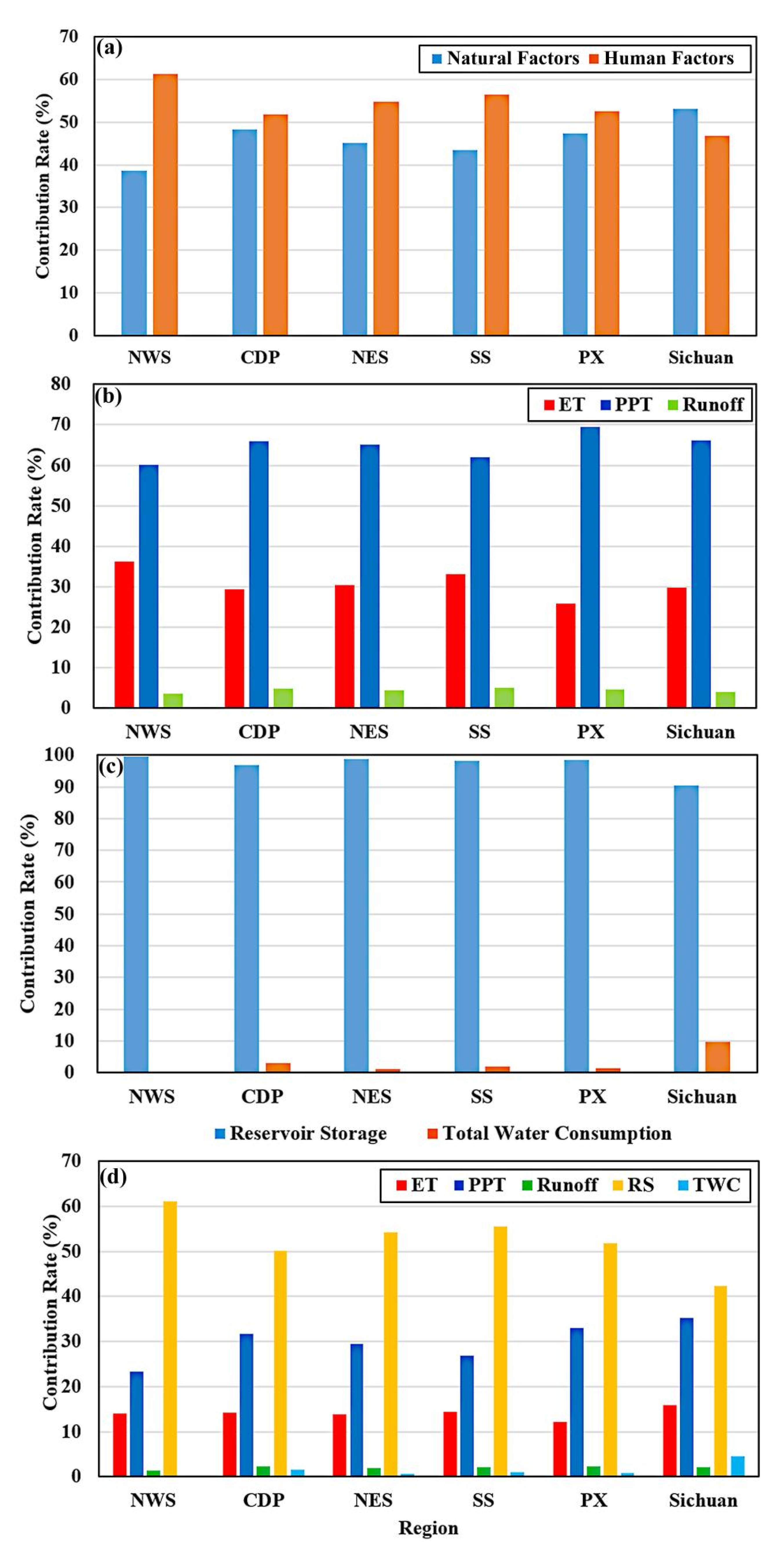
According to Equation (22), we calculated the contribution rate (CR) of natural and human factors to TWSC in Sichuan and its five economic regions (Figure 11). A larger CR means a more significant influence of this factor on TWSC. Figure 11a shows the contribution rates of TWSCc and TWSCh to TWSC and indicates that the natural influence on TWSC (CR = 53.17%) was more than the human one (CR = 46.83%) in Sichuan, but the CR of the two were not very different. However, the human influence was significantly greater than the natural one in the five economic regions. This may be because the regional divisions are based on socioeconomic development.

Figure 11.
Contribution rate of different factors from climate change and human activities to TWSC, TWSCc, and TWSCh in Sichuan and its five economic zones. RS: reservoir storage; TWC: total water consumption. (a) CR of natural and human factors to TWSC; (b) CR of PPT, ET and runoff to TWSCc; (c) CR of reservoir storage and total water consumption to TWSCh; (d) CR of PPT, ET, runoff, reservoir storage and total water consumption to TWSC.
Among the five regions, the CR of natural factors was the smallest (38.63%) and that of human factors was the largest (61.37%) in NWS. This is because this region is located in the transition region between the Sichuan Basin and Qinghai–Tibet Plateau, so there are abundant hydropower resources. Therefore, reservoir storage has a great influence on TWSC in this region. Figure 11c shows that the CR of reservoir storage to TWSC was 99.58%, which was the largest in the five regions. There was little PPT all year in NWS [64,65] because PPT was the natural factor with the largest contribution to TWSC in the five economic regions (CR > 60%, Figure 11b). Figure 11b shows that the CR of PPT to TWSCc was the smallest in NWS (60.17%). The region with the largest CR of human factors to TWSC (48.21%) was CDP because CDP is the most economically developed and densely populated region in Sichuan [66] (Table 9). Figure 11c shows that the CR of total water consumption to TWSCH (3.03%) was the highest in CDP.
Table 9.
Statistics of GDP and resident population of Sichuan and its five economic regions (data from 2019).
These five economic regions were sorted in ascending order of CR of human factors to TWSC, and their arrangement was NWS (61.37%), SS (56.49%), NES (54.85%), PX (52.6%), and CDP (51.79%). From Figure 11c, CRs of reservoir storage to TWSCH were greater than 96% in the five economic regions and explains that the reason human factors had a greater influence on TWSC than natural factors in Sichuan was reservoir storage. Figure 11d shows that the CR of reservoir storage was much greater than that of natural factors (PPT, ET, and runoff). This is because Sichuan is a province with large hydropower resources in China and one of the starting points of the West–East Power Transmission Project. The proportion of hydropower generation in Sichuan is about 82.83% [57]. Similarly, according to the CR of natural factors to TWSC, the order of the five economic regions was CDP (48.21%), PX (47.4%), NES (45.15%), SS (43.51%), and NWS (38.63%). Figure 11b shows that the CRs of PPT to TWSCC were greater than 60% in the five economic regions and explains that PPT had a greater influence on TWSCC than ET and runoff. Therefore, the CR of natural factors to TWSC mainly depends on PPT.
From Figure 11b, PPT had the highest CR to TWSCc, followed by ET and runoff in all regions. The same result was also obtained from Figure 11d without considering the CR of reservoir storage. Figure 11c shows the CR of reservoir storage and total water consumption to TWSCh. We found that except for CDP, CRs of reservoir storage to TWSCh in the other five regions were close because CDP belongs to the plains, while the other four regions belong to the mountains [5]. Therefore, there are more abundant hydropower resources in the above four regions. These five economic regions were sorted in ascending order of CR of total water consumption to TWSC, and their arrangement was CDP (3.03%), SS (1.83%), PX (1.47%), NES (1.25%), and NWS (0.42%). This order was similar to the GDP ranking of the five economic regions, and the difference was the order of PX and NES (Table 9). From Figure 11c and Table 9, the GDP of NES was greater than that of PX, but the CR of total water consumption to TWSCh in PX was higher than that in NES because PX is the most abundant vanadium and titanium ore resource and one of the four major iron ore regions in China, and the mining and processing of metal ore require a lot of water resources [67]. Figure 11b,c only considered the most influential factor on TWSCc and TWSCh, respectively. We need to further analyze the influence of different natural and human factors on TWSC in the research regions. From Figure 11d, we found that the CR of reservoir storage was the highest, followed by PPT, ET, runoff, and total water consumption in the five economic regions. From the perspective of the whole of Sichuan, the CR of total water consumption was greater than that of runoff.
6. Discussion
According to the description in Figure 11d, reservoir storage is the largest contribution to TWSC in the five economic regions and the entire Sichuan region. Therefore, reservoir storage is something we must pay attention to when studying the mechanism of TWSC. Tian et al. [68] indicated that the implementation of the Three Gorges Project has led to the increase in TWSC in the Three Gorges Reservoir region, and its growth rate was 15~20 mm/a between 2002 and 2016. Xie et al. [4] suggests that Longyangxia Reservoir and Xiaolangdi Reservoir have a very significant influence on TWSC in the region. The contributions of reservoir storage to TWSC in the regions where the Longyangxia Reservoir and Xiaolangdi Reservoir are located are significantly greater than those in the other regions of Yellow River Basin. However, in the research of hydrological disasters (floods and drought), more attention is paid to the influence of natural factors, and less research has been conducted on the role of human activities. Therefore, we will focus on the role of human factors (especially reservoir storage) in the formation of hydrological disasters in our next study.
The relevant data about human activities in this study were mainly from the Sichuan Provincial Water Resources Bulletin, which is a comprehensive annual report on the situation of water resources in Sichuan Province issued by the Sichuan Provincial Department of Water Resources. Therefore, these data have high reference value and reliability. However, the temporal resolution of these data is relatively low, all of which are annual values. It has certain limitations in the study on the influence of human activities on TWSC in this study. Therefore, it was the focus of our work to obtain monthly data on human activities in follow-up research, which will help us to more accurately understand the complex underlying mechanism for TWSC.
7. Conclusions
With global warming and the rapid development of human society and economy, the TWS in Sichuan has undergone tremendous change in the past decade. For a comprehensive understanding of the mechanisms affecting TWSC, we used GRACE/GRACE-FO satellite data to study the spatial and temporal change of TWS in Sichuan from 2003 to 2020. To improve the reliability of TWSC results, we fused TWSC results from six GRACE/GRACE-FO solutions by using the GTCH and least square methods. We analyzed the influence of natural and human factors on TWSC in Sichuan. The results showed that TWSC in Sichuan has undergone a significant increase at a rate of 3.83 ± 0.54 mm/a during the study period. For natural factors, the CR of PPT to TWSCc (66.13%) was the largest, followed by ET and runoff; for human factors, the CR of reservoir storage to TWSCh (90.38%) was the largest, followed by total water consumption; for all factors, the CR of reservoir storage to TWSC (43.32%) was the largest, followed by PPT, ET, total water consumption, and runoff. Overall, the influence of natural factors on TWSC was greater than that of human factors in the entire Sichuan region.
With the rapid development of human society, the phenomenon of water shortage and uneven distribution will become more and more serious, especially in densely populated regions. Our study will help the public understand the mechanism of TWS variations and provide valuable information for decisions-makers in making the right policies for water resource scheduling and protection.
Author Contributions
Conceptualization, L.C. and J.A.; Methodology, J.A. and C.Y.; Software, C.Z.; Validation, L.C., C.Y. and Y.W.; Formal analysis, X.W.; Resources, L.C. and P.W.; Data duration, C.Z. and L.C.; Writing—original draft preparation, L.C.; Writing—review and editing, L.C., Y.W. and X.W.; Funding acquisition, Y.W. All authors have read and agreed to the published version of the manuscript.
Funding
This research was funded by the National Natural Science Fund of China (41974096, 41931074, 42171141, 42004013), the Foundation of Young Creative Talents in Higher Education of Guangdong Province (2019KQNCX009), and the Guangzhou Science and Technology Project (202102020526).
Institutional Review Board Statement
Not applicable.
Informed Consent Statement
Not applicable.
Data Availability Statement
GRACE RL06 data from CSR, GFZ, JPL, and ITSG: http://icgem.gfz-potsdam.de/series (accessed on 10 January 2022); In situ precipitation data: http://data.cma.cn (accessed on 10 January 2022); ET gridded data: sftp://hydras.ugent.be (accessed on 10 January 2022); Reconstructed TWSC data: http://data.tpdc.ac.cn (accessed on 10 January 2022); Human-induced TWSC data: http://slt.sc.gov.cn/ (accessed on 10 January 2022).
Acknowledgments
We are grateful to CSR, GFZ, and JPL for providing the monthly GRACE gravity field solution; the Goddard Space Flight Center for providing the monthly GLDAS-2.1 data; the China National Meteorological Science Data Center for providing the monthly precipitation products; the Global Land Evaporation Amsterdam Model for providing the ET data; the National Tibetan Plateau Data for providing the dataset of reconstructed terrestrial water storage in China based on precipitation (2002–2019); and to the Sichuan Provincial Department of Water Resources for providing the Sichuan Province Water Resources Bulletin.
Conflicts of Interest
The authors declare no conflict of interest.
References
- WMO; UNESCO. International Glossary of Hydrology, 3rd ed.; WMO: Genève, Switzerland, 2012; pp. 377–378. [Google Scholar]
- Tapley, B.D.; Watkins, M.M.; Flechtner, F.; Reigber, C.; Bettadpur, S.; Rodell, M.; Sasgen, I.; Famiglietti, J.S.; Landerer, F.W.; Chambers, D.P.; et al. Contributions of GRACE to understanding climate change. Nat. Clim. Chang. 2019, 9, 358–369. [Google Scholar] [CrossRef]
- Nanteza, J.; De Linage, C.R.; Thomas, B.F.; Famiglietti, J.S. Monitoring groundwater storage changes in complex basement aquifers: An evaluation of the GRACE satellites over East Africa. Water Resour. Res. 2016, 52, 9542–9564. [Google Scholar] [CrossRef]
- Xie, J.; Xu, Y.-P.; Wang, Y.; Gu, H.; Wang, F.; Pan, S. Influences of climatic variability and human activities on terrestrial water storage variations across the Yellow River basin in the recent decade. J. Hydrol. 2019, 579, 124218. [Google Scholar] [CrossRef]
- Ma, L.; Tang, H.; Ran, R.P.; Xiao, Y.J. Study on spatial and temporal evolvement and coupling effect of water resources pressure and cultivated land use efficiency in Sichuan. Chin. J. Agric. Resour. Reg. Plan. 2019, 40, 9–19. (In Chinese) [Google Scholar]
- Sichuan Provincial Bureau of Statistics; National Bureau of Statistics Sichuan Investigation Team. Sichuan Statistical Yearbook 2020; China Statistics Press: Beijing, China, 2020; pp. 20–25. [Google Scholar]
- Cao, K. Analysis and forecast of climate and water resources changes in Sichuan. Northeast. Water Resour. Hydropower 2018, 4, 28–30. (In Chinese) [Google Scholar]
- Cui, L.; Zhang, C.; Yao, C.; Luo, Z.; Wang, X.; Li, Q. Analysis of the Influencing Factors of Drought Events Based on GRACE Data under Different Climatic Conditions: A Case Study in Mainland China. Water 2021, 13, 2575. [Google Scholar] [CrossRef]
- Chahine, M.T. The hydrological cycle and its influence on climate. Nature 1992, 359, 373–380. [Google Scholar] [CrossRef]
- Liljedahl, A.K.; Hinzman, L.D.; Kane, D.L.; Oechel, W.C.; Tweedie, C.E.; Zona, D. Tundra water budget and implications of precipitation underestimation. Water Resour. Res. 2017, 53, 6472–6486. [Google Scholar] [CrossRef] [Green Version]
- Anyah, R.O.; Forootan, E.; Awange, J.L.; Khaki, M. Understanding linkages between global climate indices and terrestrial water storage changes over Africa using GRACE products. Sci. Total Environ. 2018, 635, 1405–1416. [Google Scholar] [CrossRef] [Green Version]
- Banerjee, C.; Sharma, A. Decline in terrestrial water recharge with increasing global temperatures. Sci. Total Environ. 2021, 764, 142913. [Google Scholar] [CrossRef]
- Wang, D.; Cai, X. Detecting human interferences to low flows through base flow recession analysis. Water Resour. Res. 2009, 45, 07426. [Google Scholar] [CrossRef]
- Yang, Y.; Weng, B.; Man, Z.; Yu, Z.; Zhao, J. Analyzing the contributions of climate change and human activities on runoff in the Northeast Tibet Plateau. J. Hydrol. Reg. Stud. 2020, 27, 100639. [Google Scholar] [CrossRef]
- Joodaki, G.; Wahr, J.; Swenson, S. Estimating the human contribution to groundwater depletion in the Middle East, from GRACE data, land surface models, and well observations. Water Resour. Res. 2014, 50, 2679–2692. [Google Scholar] [CrossRef]
- Felfelani, F.; Wada, Y.; Longuevergne, L.; Pokhrel, Y.N. Natural and human-induced terrestrial water storage change: A global analysis using hydrological models and GRACE. J. Hydrol. 2017, 553, 105–118. [Google Scholar] [CrossRef] [Green Version]
- Feng, W.; Zhong, M.; Lemoine, J.-M.; Biancale, R.; Hsu, H.-T.; Xia, J. Evaluation of groundwater depletion in North China using the Gravity Recovery and Climate Experiment (GRACE) data and ground-based measurements. Water Resour. Res. 2013, 49, 2110–2118. [Google Scholar] [CrossRef]
- Cui, L.; Zhang, C.; Luo, Z.; Wang, X.; Li, Q.; Liu, L. Using the Local Drought Data and GRACE/GRACE-FO Data to Characterize the Drought Events in Mainland China from 2002 to 2020. Appl. Sci. 2021, 11, 9594. [Google Scholar] [CrossRef]
- Singh, A.; Reager, J.T.; Behrangi, A. Estimation of hydrological drought recovery based on precipitation and Gravity Recovery and Climate Experiment (GRACE) water storage deficit. Hydrol. Earth Syst. Sci. 2021, 25, 511–526. [Google Scholar] [CrossRef]
- Chen, J.L.; Wilson, C.R.; Tapley, B. The 2009 exceptional Amazon flood and interannual terrestrial water storage change observed by GRACE. Water Resour. Res. 2010, 46, 12526. [Google Scholar] [CrossRef] [Green Version]
- Li, Q.; Luo, Z.; Zhong, B.; Zhou, H. An Improved Approach for Evapotranspiration Estimation Using Water Balance Equation: Case Study of Yangtze River Basin. Water 2018, 10, 812. [Google Scholar] [CrossRef] [Green Version]
- Long, D.; Chen, X.; Scanlon, B.R.; Wada, Y.; Hong, Y.; Singh, V.P.; Chen, Y.N.; Wang, C.G.; Han, Z.Y.; Yang, W.T. Have GRACE satellites overestimated groundwater depletion in the Northwest India Aquifer? Sci. Rep. 2016, 6, 24398. [Google Scholar] [CrossRef]
- Eom, J.; Seo, K.-W.; Ryu, D. Estimation of Amazon River discharge based on EOF analysis of GRACE gravity data. Remote Sens. Environ. 2017, 191, 55–66. [Google Scholar] [CrossRef]
- Willen, M.O.; Horwath, M.; Schröder, L.; Groh, A.; Ligtenberg, S.R.M.; Munneke, P.K.; Broeke, M.R.V.D. Sensitivity of inverse glacial isostatic adjustment estimates over Antarctica. Cryosphere 2020, 14, 349–366. [Google Scholar] [CrossRef] [Green Version]
- Zou, F.; Tenzer, R.; Fok, H.; Nichol, J. Recent Climate Change Feedbacks to Greenland Ice Sheet Mass Changes from GRACE. Remote Sens. 2020, 12, 3250. [Google Scholar] [CrossRef]
- Yi, S.; Sun, W.K.; Feng, W.; Chen, J.L. Anthropogenic and climate-deiven water depletion in Asia. Geophys. Res. Lett. 2016, 43, 9061–9069. [Google Scholar] [CrossRef]
- Chen, H.; Liu, H.; Chen, X.; Qiao, Y. Analysis on impacts of hydro-climatic changes and human activities on available water changes in Central Asia. Sci. Total Environ. 2020, 737, 139779. [Google Scholar] [CrossRef]
- Zhang, B.; Liu, L.; Yao, Y.; van Dam, T.; Khan, S.A. Improving the estimate of the secular variation of Greenland ice mass in the recent decades by incorporating a stochastic process. Earth Planet. Sci. Lett. 2020, 549, 116518. [Google Scholar] [CrossRef]
- Chen, C.; Pang, Y.M.; Zhang, Y.F.; Chen, D.D. Study on the sensitivity and vulnerability of winter wheat yield to climate change in Sichuan province. J. Nat. Res. 2017, 32, 127–136. (In Chinese) [Google Scholar]
- Swenson, S.; Chambers, D.; Whar, J. Estimating geocenter variations form a combination of GRACE and ocean model output. J. Geophys. Res Solid Earth 2008, 113, 194–205. [Google Scholar]
- Cheng, M.; Tapley, B. Variations in the Earth’s oblateness during the past 28 years. J. Geophys. Res. Earth Surf. 2004, 109, 09402. [Google Scholar] [CrossRef]
- Cui, L.; Song, Z.; Luo, Z.; Zhong, B.; Wang, X.; Zou, Z. Comparison of Terrestrial Water Storage Changes Derived from GRACE/GRACE-FO and Swarm: A Case Study in the Amazon River Basin. Water 2020, 12, 3128. [Google Scholar] [CrossRef]
- Zhong, Y.L.; Feng, W.; Zhong, M.; Ming, Z.T. Dataset of Reconstructed Terrestrial Water Storage in China Based on Precipitation (2002–2019); National Tibetan Plateau Data Center: Beijing, China, 2020. [Google Scholar] [CrossRef]
- Zhong, Y.; Feng, W.; Humphrey, V.; Zhong, M. Human-Induced and Climate-Driven Contributions to Water Storage Variations in the Haihe River Basin, China. Remote Sens. 2019, 11, 3050. [Google Scholar] [CrossRef] [Green Version]
- Rodell, M.; Houser, P.R.; Jambor, U.; Gottschalck, J.; Mitchell, K.; Meng, C.-J.; Arsenault, K.; Cosgrove, B.; Radakovich, J.; Bosilovich, M.; et al. The Global Land Data Assimilation System. Bull. Am. Meteorol. Soc. 2004, 85, 381–394. [Google Scholar] [CrossRef] [Green Version]
- Miralles, D.G.; Holmes, T.R.H.; De Jeu, R.A.M.; Gash, J.H.; Meesters, A.G.C.A.; Dolman, A.J. Global land-surface evaporation estimated from satellite-based observations. Hydrol. Earth Syst. Sci. 2011, 15, 453–469. [Google Scholar] [CrossRef] [Green Version]
- Martens, B.; Gonzalez Miralles, D.; Lievens, H.; Van Der Schalie, R.; De Jeu, R.A.M.; Fernández-Prieto, D.; Beck, H.E.; Dorigo, W.A.; Verhoest, N.E.C. GLEAM v3: Satellite-based land evaporation and root-zone soil moisture. Geosci. Model Dev. 2017, 10, 1903–1925. [Google Scholar] [CrossRef] [Green Version]
- Sichuan Hydrology and Water Resources Survey Bureau. Sichuan Province Water Resources Bulletin; Sichuan Provincial Water Resources Department: Chengdu, China, 2020. [Google Scholar]
- Yao, C.L.; Li, Q.; Luo, Z.C.; Wang, C.R.; Zhang, R.; Zhou, B.Y. Uncertainties in GRACE-derived terrestrial water storage changes over mainland China based on a generalized three-cornered hat method. Chines J. Geophys. 2019, 62, 883–897. (In Chinese) [Google Scholar]
- Tavella, P.; Premoli, A. Estimating the instabilities of N clock by measuring differences of their readings. Metrologia 1994, 30, 479–486. [Google Scholar] [CrossRef]
- Galindo, F.J.; Palacio, J. Post-processing ROA data clocks for optimal stability in the ensemble timescale. Metrologia 2003, 40, S237–S244. [Google Scholar] [CrossRef]
- Galindo, F.J.; Palacio, J. Estimating the instabilities of N correlated clocks. In Proceedings of the 31st Annual Precise Time and Time Interval (PTTI) Meeting, Real Instituto y Observatorio de la, Dana Point, CA, USA, 7–9 December 1999; pp. 285–296. [Google Scholar]
- Premoli, A.; Tavella, P. A revisited three-cornered hat method for estimating frequency standard instability. IEEE Trans. Instrum. Meas. 1993, 42, 7–13. [Google Scholar] [CrossRef]
- Koot, L.; Viron, O.D.; Dehant, V. Atmospheric Angular Momentum Time-Series: Characterization of their Internal Noise and Creation of a Combined Series. J. Geodesy 2006, 79, 663–674. [Google Scholar] [CrossRef]
- Cui, L.; Luo, C.; Yao, C.; Zou, Z.; Wu, G.; Li, Q.; Wang, X. The Influence of Climate Change on Forest Fires in Yunnan Province, Southwest China Detected by GRACE Satellites. Remote Sens. 2022, 14, 712. [Google Scholar] [CrossRef]
- Kim, H.; Yeh, P.J.-F.; Oki, T.; Kanae, S. Role of rivers in the seasonal variations of terrestrial water storage over global basins. Geophys. Res. Lett. 2009, 36, 17402. [Google Scholar] [CrossRef] [Green Version]
- Wu, H.B. Studies on glacier mass balance in the High Asia retrieved by ICESat-GLAS data and GRACE time-varying gravity field. Acta Geod. Cartogr. Sin. 2020, 49, 534. [Google Scholar]
- Wei, L.; Dan, B.; Wang, F.; Fu, B.; Yan, J.; Shuai, W.; Yang, Y.; Di, L.; Feng, M. Quantifying the impacts of climate change and ecological restoration on streawflow changes based on a Budyko hydrological model in China’s Loess Plateau. Water Resour. Res. 2015, 51, 6500–6519. [Google Scholar]
- Yang, Y.; Shang, S.; Jiang, L. Remote sensing temporal and spatial patterns of evapotranspiration and the responses to water management in a large irrigation district of North China. Agric. For. Meteorol. 2012, 164, 112–122. [Google Scholar] [CrossRef]
- Scanlon, B.R.; Zhang, Z.; Save, H.; Sun, A.Y.; Schmied, H.M.; van Beek, L.P.H.; Wiese, D.N.; Wada, Y.; Long, D.; Reedy, R.C.; et al. Global models underestimate large decadal declining and rising water storage trends relative to GRACE satellite data. Proc. Natl. Acad. Sci. USA 2018, 115, E1080–E1089. [Google Scholar] [CrossRef] [Green Version]
- Yao, C.L. Natural- and Human-Induced Impacts on Regional Terrestrial Water Storage Changes from GRACE and Hyd-MeteOrological Data. Ph.D. Thesis, Wuhan University, Wuhan, China, 2017. (In Chinese). [Google Scholar]
- Wang, C.Y. Deficiency of China’s water conservation legislation and improvement proposals. J. Shenzhen Univ. 2020, 37, 87–96. [Google Scholar]
- Yi, S.; Song, C.; Wang, Q.; Wang, L.; Heki, K.; Sun, W. The potential of GRACE gravimetry to detect the heavy rainfall-induced impoundment of a small reservoir in the upper Yellow River. Water Resour. Res. 2017, 53, 6562–6578. [Google Scholar] [CrossRef]
- Xie, Y.; Huang, S.Z.; Liu, S.Y.; Leng, G.Y.; Peng, J.; Huang, Q.; Li, P. GRACE-based terrestrial water storage in Northwest China: Changes and causes. Remote. Sens. 2018, 10, 1163. [Google Scholar] [CrossRef] [Green Version]
- Wang, X.; De Linage, C.; Famiglietti, J.; Zender, C.S. Gravity Recovery and Climate Experiment (GRACE) detection of water storage changes in the Three Gorges Reservoir of China and comparison with in situ measurement. Water Resour. Res. 2011, 47, 010534. [Google Scholar] [CrossRef]
- Li, Y.G.; Li, L.; Li, G.W. Research on the development value of Sichuan hydropower station under the new situation. Hydropower Stn. Des. 2019, 35, 67–69. (In Chinese) [Google Scholar]
- Sun, H.L.; Wang, D.; Wu, Y.Y.; Jin, L.X.; Liu, W.J. Analysis for the effect of hydropower and water conservancy engineering on basin eco-environment in the Upper Yangtze River. Environ. Prot. 2017, 45, 37–40. (In Chinese) [Google Scholar]
- Kong, D.; Miao, C.; Wu, J.; Duan, Q.; Sun, Q.; Ye, A.; Di, Z.; Gong, W. The hydro-environmental response on the lower Yellow River to the water–sediment regulation scheme. Ecol. Eng. 2015, 79, 69–79. [Google Scholar] [CrossRef]
- Bulletin of Seventh National Population Census (No.3). Available online: http://www.stats.gov.cn/tjsj/tjgb/rkpcgb/qgrkpcgb/2-02106/t20210628_1818822.html (accessed on 10 January 2022).
- Statistical Bureau of Sichuan. NBS Survey Office in Sichuan. Sichuan Statistical Yearbook; China Statistical Press: Beijing, China, 2020; pp. 3–5. [Google Scholar]
- Ibrahim, M.; Favreau, G.; Scanlon, B.R.; Seidel, J.L.; Le Coz, M.; Demarty, J.; Cappelaere, B. Long-term increase in diffuse groundwater recharge following expansion of rainfed cultivation in the Sahel, West Africa. Appl. Hydrogeol. 2014, 22, 1293–1305. [Google Scholar] [CrossRef]
- Werth, S.; White, D.; Bliss, D.W. GRACE Detected Rise of Groundwater in the Sahelian Niger River Basin. J. Geophys. Res. Solid Earth 2017, 122, 10459–10477. [Google Scholar] [CrossRef]
- He, Y.F. Study on Agricultural Industrial Structure of Five Economic Zones in Sichuan Province Based on DSSM Model. Master’s Thesis, Chengdu University of Technology, Chengdu, China, 2018. (In Chinese). [Google Scholar]
- Zhang, H.J. A study on the characteristics of climate change on Northwestern Sichuan Plateau. J. Southwest Univ. 2014, 36, 148–156. (In Chinese) [Google Scholar]
- Cao, J.; Shao, H.Y.; Li, B.; Zhang, X.X.; Chen, G.M.; Yang, X. Response of climate and human factor on the variation of grassland: A case study on Ruoergai County. Environ. Sci. Technol. 2017, 40, 13–18. (In Chinese) [Google Scholar]
- Duan, H.Y. Study on Coordinated Development of Economic Zone of Chengdu. Master’s Thesis, Chengdu University of Technology, Chengdu, China, 2016. (In Chinese). [Google Scholar]
- Liu, Y. Non-technical factors in the technological breakthrough of vanadium titano-magnetite smelting in Panzhihua during the Third Front Construction Period. Chin. J. Hist. Sci. Technol. 2016, 37, 473–484. [Google Scholar]
- Tian, X.J.; Zou, F.; Jin, S.G. Impact of climate change and human activities on water storage changes in the Yangtze River basin. J. Geod. Geodyn. 2019, 39, 371–377. [Google Scholar]

Publisher’s Note: MDPI stays neutral with regard to jurisdictional claims in published maps and institutional affiliations. |
© 2022 by the authors. Licensee MDPI, Basel, Switzerland. This article is an open access article distributed under the terms and conditions of the Creative Commons Attribution (CC BY) license (https://creativecommons.org/licenses/by/4.0/).