Article

Cloud–Snow Confusion with MODIS Snow Products in Boreal Forest Regions

1
College of Earth and Environmental Sciences, Lanzhou University, Lanzhou 730000, China
2
School of Geography and Ocean Science, Nanjing University, Nanjing 210000, China
3
Northwest Institute of Eco-Environment and Resources, Chinese Academy of Sciences, Lanzhou 730000, China
4
Jiangsu Center for Collaborative Innovation in Geographical Information Resource Development and Application, Nanjing 210023, China
*
Author to whom correspondence should be addressed.
Remote Sens. 2022, 14(6), 1372; https://doi.org/10.3390/rs14061372
Submission received: 31 December 2021 / Revised: 25 February 2022 / Accepted: 7 March 2022 / Published: 11 March 2022
(This article belongs to the Special Issue Remote Sensing for Mountain Vegetation and Snow Cover)

Abstract

:
Reliable cloud masks in Moderate Resolution Imaging Spectroradiometer (MODIS) snow cover products have a high potential to improve the retrieval of snow properties. However, cloud–snow confusion is a popular problem in MODIS snow cover products, especially in boreal forest areas. A large amount of forest snow is misclassified as clouds because of the low normalized difference snow index (NDSI), and excessive cloud masks limit the application of snow products. In addition, ice clouds are easily misclassified as snow due to their similar spectral characteristics, which leads to snow commission errors. In this paper, we quantitatively evaluated the cloud–snow confusion in Northeast China and found that snow-covered forests and transition zones from snow-covered to snow-free areas are prone to being misclassified as clouds, while clouds are less likely to be misclassified as snow. A temporal-sequence cloud–snow-distinguishing algorithm based on the high-frequency observation characteristics of the Himawarri-8 geostationary meteorological satellite is proposed. In the temporal-sequence images acquired from that satellite, the NDSI variance in cloud pixels should be greater than that of snow because clouds vary over time, while snow is relatively stable. In the MODIS snow cover products, the cloud pixels with NDSI variance lower than a threshold are identified as cloud-free areas and attributed their raw NDSI value, while the snow pixels with NDSI variance greater than the threshold are marked as clouds. We applied this method to MOD10A1 C6 in Northeast China. The results showed that the excessive cloud masks were greatly eliminated, and the new cloud mask was in good agreement with the real cloud distribution. At the same time, some possible ice clouds which had been misclassified as snow for their spectral characteristics similar to those of snow were identified correctly.

Graphical Abstract

1. Introduction

Snow cover is a key component of the cryosphere; it plays an important role in global energy balance and atmospheric circulation due to its high albedo and low thermal conductivity [1,2,3]. The large-scale expansion and retreat of snow cover can greatly change the weather and climate system [4,5]. Compared with the limited amount of in situ measurements provided by sparse meteorological stations, remote sensing technology can produce spatiotemporal patterns of snow cover on a larger scale [6,7]. Among the current remote sensing products of snow cover, the Moderate Resolution Imaging Spectroradiometer (MODIS) daily snow cover products have been extensively employed owing to their relatively high temporal (1 day) and spatial (500 m) resolution, as well as their long duration [8,9,10,11,12,13]. Cloud cover is inevitable in optical remote sensing, and some literature shows that, on average, clouds cover more than half of the Earth’s surface every day [14,15,16,17]. Due to cloud cover, the current MODIS snow cover products are spatially and temporally incomplete, which affects their application.
The new version (version 6, referred to as C6) of MODIS snow cover products was released in 2014. MODIS snow products C6 are focused on improving snow detection in clear sky conditions [18]. The unobstructed Filed of View (UFOV) cloud mask flag from MOD35_L2 is used to mask clouds for MOD/MYD10A1. The pixels which are flagged “certain cloud” are marked as cloud, while “confident clear”, “probably clear”, or “uncertain clear” are interpreted as clear [19]. Although some minor improvements were made in the C6 cloud mask product, there is still serious cloud–snow confusion in some situations. Clouds are brighter and colder than most land surfaces, and the existing cloud masking algorithms are usually effective. However, cloud masking algorithms perform the worst in snow-covered areas, where some clouds are identified as snow, and some snow is identified as cloud [2]. The 1.38 µm band in MODIS is used for the detection of thin cirrus [20,21], but it is difficult to detect thin cirrus in high albedo surfaces, such as snow [22]. A characteristic of snow are its very high visible (VIS) reflectance and very low reflectance in the shortwave–infrared (SWIR) region; the SWIR reflectance of clouds is higher than that of snow. Therefore, the normalized difference snow index (NDSI), which is defined as NDSI = (Rgreen − Rswir)/(Rgreen + Rswir), is incorporated into the MODIS cloud mask to distinguish snow from most cloud types; Rgreen and Rswir are the reflectance of green band and SWIR band, respectively. In the presence of snow or ice, when the NDSI values are greater than a predetermined threshold, these surfaces are deemed snow- or ice-covered [23].
Stillinger et al. [24] assessed errors in cloud masks over snow-covered regions and found that the overall precision and recall of the MODIS surface reflectance product MOD09GA cloud mask were 0.17 and 0.72, respectively. Cao et al. [25] compared the clouds in Terra MODIS C5 with data from meteorological stations in China. The deviation varied with latitude and season, and it was greatest in winter; the deviation was greater than 40% in mid-latitude regions. Ma et al. [26] compared MODIS-retrieved and ground-based cloud fractions over China and found that the correlation of these two datasets was different for different underlying surfaces. Analyses without winter data led to a significantly increased correlation in Northern China. In northeastern forest areas, the correlation throughout a month is −0.186 between the ground-based cloud fraction and the MODIS cloud fraction, and the former is significantly lower than the latter. However, the correlation increases to 0.813 if the statistic is performed only for the period from April to October. Thus, the cloud mask is very unreliable in winter, especially in forest areas, which is mainly caused by the confusion between clouds and snow.
Cloud–snow distinction is always a challenging problem due to their similar spectrum characteristics. In some cases, cloud–snow detection is performed under the classification paradigm, such as support vector machine (SVM) and random forest [27,28]. The NDSI is commonly used to separate clouds from snow because snow typically has a higher NDSI than clouds [29,30,31]. Despite the wide applications of NDSI, this method has some limitations. It heavily relies on the reflectance of the imagery band and on predefined thresholds, a lack flexibility and robustness under complex scenarios such as in the presence of patchy snow or at the edge of snow areas. At high latitudes, band reflectance will decrease due to low solar elevation. In forest areas, the NDSI value of mixed pixels with canopy and snow is much less than that of pure snow pixels [32,33,34]. In recent years, deep neural networks have greatly promoted cloud and snow detection research by remote sensing [35], but these methods are difficult to use widely because they rely on too many samples, and calculations are very complicated.
Spatiotemporal continuous snow cover products are necessary for snow cover change research. Popular methods to fill the cloud gaps in the MODIS snow cover product include temporal-spatial filtering methods [36,37,38,39], adjacent temporal composite methods [40,41], and multisource fusion methods in which the cloud pixels are filled with the microwave snow water equivalent (SWE) or snow depth data [42,43,44]. Recently, some new gap-filling methods have been developed, such as methods based on similar pixels [45,46,47], time–space cubes [48], and conditional probability interpolation [49,50]. The basic idea of these cloud removal methods is to fill the value of pixels under the cloud with cloud-free pixels in the spatiotemporal neighborhood. Therefore, it is necessary to obtain a reliable cloud mask to reduce the confusion between clouds and snow.
In this paper, we took the Northeast China snow area as an example, quantitatively evaluated the cloud–snow confusion in this region, and propose a temporal-sequence cloud–snow-distinguishing algorithm based on the high-frequency observation characteristics of the Himawarri-8 geostationary meteorological satellite. Section 2 describes the study area and the datasets, Section 3 evaluates the cloud–snow confusion, Section 4 presents the cloud–snow identification methodology, and Section 5 reports the method validation and a discussion of the results. Finally, Section 6 provides the conclusions of this article.

2. Study Area and Data
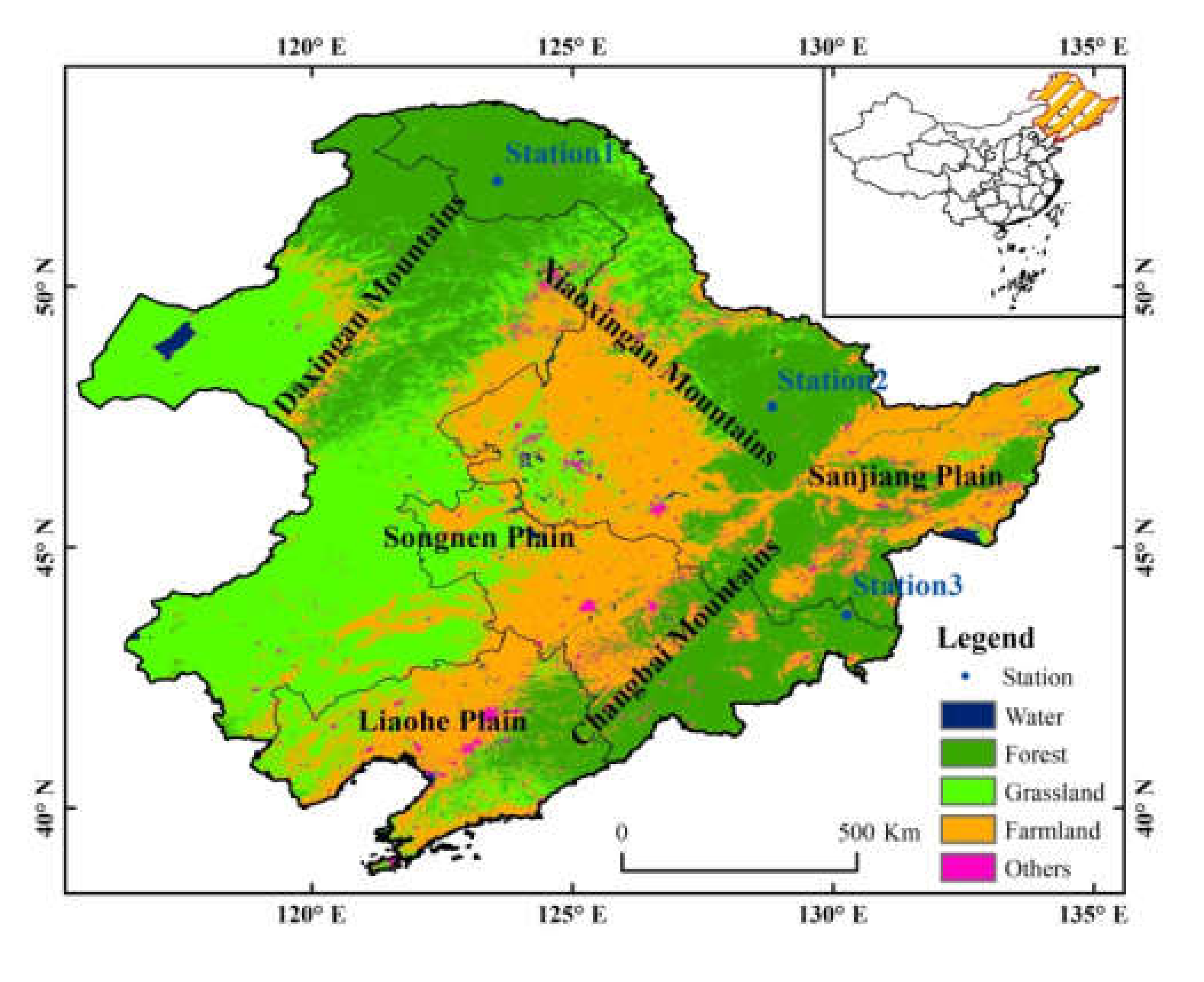
2.1. Study Area

The study area is located in Northeast China, and the sites comprise a seasonally snow-covered boreal forest. Northeast China is one of the three primary snow-covered regions in China [51]. In this area, the seasonal snow cover usually lasts from November to March of the following year. The latitude of the study area is from 38°42′N to 53°36′N, and boreal forests are widespread in the region, especially in the Daxing’an Mountains, Xiaoxing’an Mountains, and Changbai Mountains [52]. The study area is shown in Figure 1. The high latitude corresponds to the low solar elevation in winter. In the MODIS snow cover products of this region, the high forest coverage and low solar elevation lead to serious cloud–snow confusion.

2.2. MODIS/Terra Snow Cover Product MOD10A1 C6

In MOD10A1 C6, the daily snow cover is given as the NDSI_Snow_Cover data array. In version 6, compared to the previous versions, the snow cover extent binary map is deleted, and the fractional snow cover (FSC) is no longer calculated. The NDSI_Snow_Cover data are the result of the NDSI-snow detection algorithm with the cloud mask, ocean mask, and night mask overlaid. The valid NDSI codes are within the range 0–100, which is the NDSI value multiplied by 100, indicating that some snow exists in the pixels [18]. The meaning of all the codes in NDSI_Snow_Cover is shown in Table 1. Another layer of MOD10A1 is Raw_NDSI, which gives the NDSI value of each pixel.
Snow typically has high VIS reflectance and low SWIR reflectance, and the NDSI which is defined based on the difference of these two bands, is effective in detecting snow under clear and good illumination. To alleviate snow commission errors, several data screens based on snow spectral features or other characteristics are applied in the MODIS snow cover product algorithm. The first screen is a low-reflectance screen. To separate snow from water, the pixels with a reflectance of the near-infrared (NIR) band <0.11 would not pass the screening test. Those with a reflectance of the green band <0.1 will also fail in the screen tests to prevent the detection of dark targets with high NDSI values as snow [53]. The reflectance screen is usually effective; however, the amount of reflectance in any band varies depending on viewing conditions and surface features. In addition, low-NDSI screening tests are employed, pixels with 0 < NDSI < 0.1 are defined as no snow, and the value is set to be 0 in the NDSI_Snow_Cover data array. Solar zenith screen and illumination conditions are also set as screens. When the solar zenith angles >70, the corresponding illumination conditions are poor, and snow detection is challenging. These screens are significant for global snow production but will result in great snow omission errors in high-altitude boreal forest areas.

2.3. MODIS Surface Reflectance Product MOD09GA

The MOD09GA Version 6 product provides an estimate of the surface spectral reflectance of Terra MODIS Bands 1 through 7, corrected for atmospheric conditions, such as gases, aerosols, and Rayleigh scattering. Table 2 shows the band parameters of MOD09GA. The reflectance layers from MOD09GA are used as the source data in many of the MODIS land products. Clouds and snow exhibit similar characteristics in the VIS band but very different characteristics in the SWIR band. With the combination of bands 2, 4, and 6, clouds (except ice clouds) and snow appear in different colors and can be visually distinguished. In this paper, MOD09GA was used to select cloud and snow samples and verify the results of cloud and snow discrimination.

2.4. Advanced Himawari Imager (AHI) Data

Himawari-8, which was launched on 7 October 2014, is the first new-generation geostationary meteorological satellite in the world. It carries a multiwavelength (from visible to infrared) imager named AHI, including the green band and the SWIR band, which are popularly used in snow cover remote sensing. The temporal resolution of all bands is 10 min. The band information is reported in Table 3. The ALI data are from https://www.eorc.jaxa.jp/ptree/ (accessed on 30 December 2021).

2.5. Gridded Climatic Research Unit Time-Series Data

The gridded Climatic Research Unit (CRU) Time-Series (TS) data version 4.04 are month-by-month variations in climate over the period of 1901–2019. These data are derived by the interpolation of monthly climate anomalies from extensive networks of weather station observations. The grid has a latitude of 0.5° and a longitude of 0.5° in all land areas of the world except Antarctica. It includes cloud cover, diurnal temperature range, frost-day frequency, wet-day frequency, potential evapotranspiration (PET), precipitation, daily mean temperature, monthly average daily maximum/minimum temperature, and vapor pressure. In this paper, we used CRU TS4.04 cloud cover data from https://data.ceda.ac.uk/badc/cru/data/cru_ts/cru_ts_4.04/data (accessed on 30 December 2021) and used them as actual cloud coverage to evaluate the cloud mask in MOD10A1 C6.

3. Cloud–Snow Confusion in MOD10A1

3.1. Cloud Mask in MOD10A1

In the NDSI_Snow_Cover data array, the cloud pixel was assigned a value of 250. To show the cloud distribution in MODIS snow cover products, the cloud cover days (CCDs) were counted for each pixel in the study area from 2014 to 2018. Figure 2 shows the average CCDs per month in Northeast China from 2014 to 2018, which were counted based on MOD10A1. The snow season in Northeast China is from November to March of the following year, and the CCDs in this period are significantly greater than in other months. Especially in forested areas, most CCDs were more than 25 in that period. The number of CCDs in September and October was the lowest of the year. From April to August, the number of CCDs in the mountainous area was slightly higher than in the plains, but it was lower than in winter. Figure 3 shows the CCDs of three stations located on Daxing’an Mountains, Xiaoxing’an Mountains, and Changbai Mountains; they were extracted from the only pixel where the station of the NDSI_Snow_Cover data array was located. The positions of these three stations are shown in Figure 1.
Figure 4 shows the average cloud coverage per month in Northeast China from 2014 to 2018, which was determined based on CRU TS4.04. This finding shows that the cloud coverage in winter was actually less than that in summer in Northeast China. The cloud coverage was highest in June, July, and August but not in January, February, and December.
A comparison of Figure 2, Figure 3 and Figure 4 shows that there were excessive cloud masks in MOD10A1 in the snow season, especially in forest areas. This result is most likely due to cloud and snow confusion, and it will be discussed in Section 5.2.

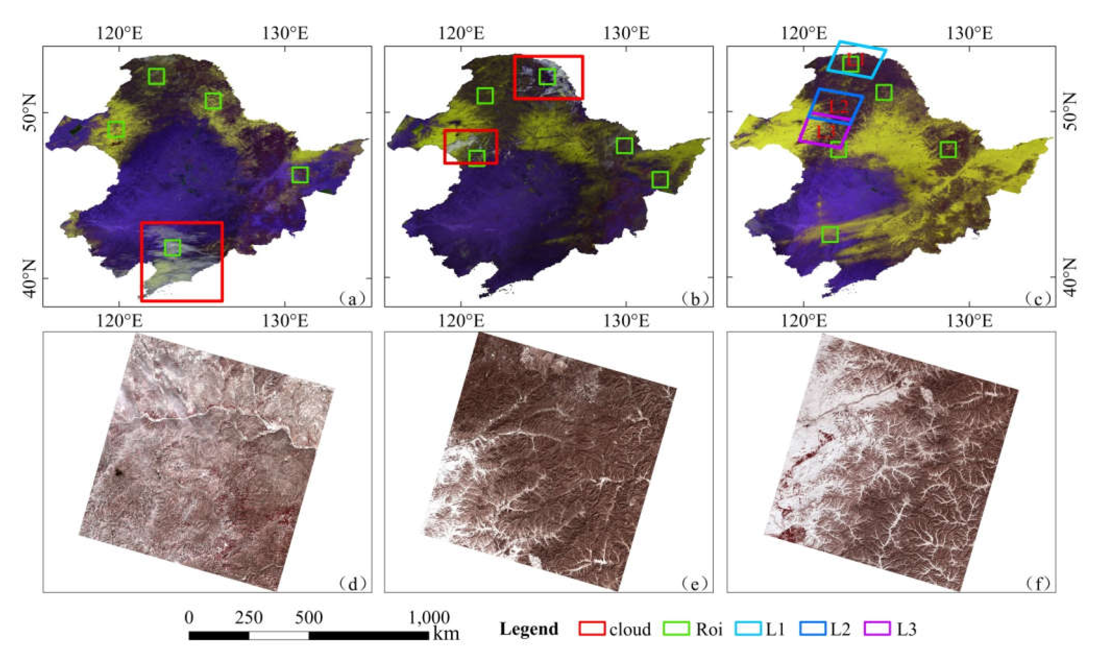
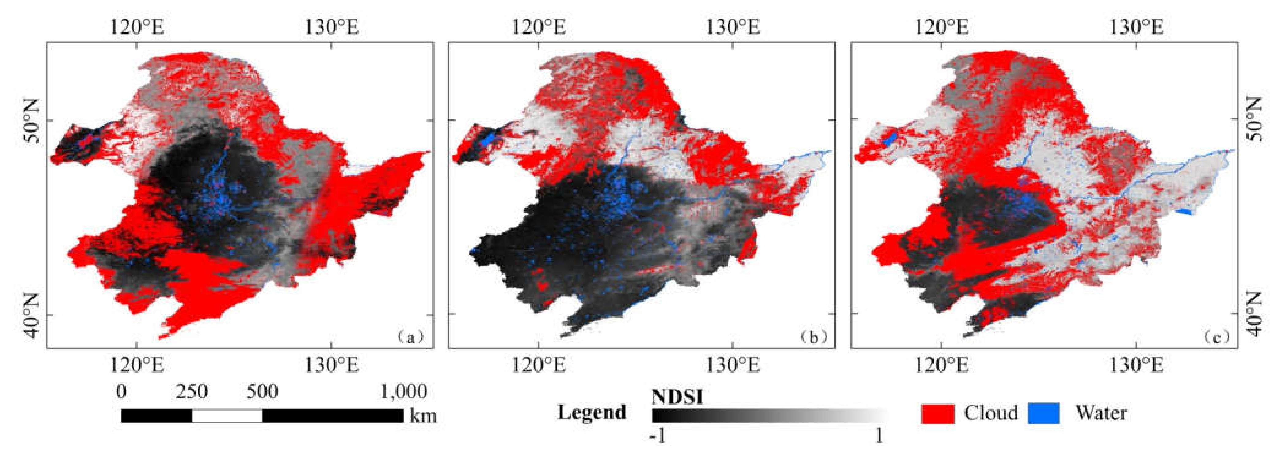
3.2. Clouds Misclassified as Snow

Clouds and snow are both bright in the visible spectral region, while in the shortwave–infrared region, small scattering elements, such as water droplets in clouds, make clouds brighter than snow [54]. This understanding is usually used to distinguish snow from clouds. However, ice clouds are made of non-spherical ice crystal particles, and their spectral properties are almost identical to those of snow [55]. Figure 5a is the false-color image combining bands 1 (red), 2 (NIR), and 4 (green) as RGB, which was acquired on 10 January 2018. In winter, there is much snow in Northeast China, so the white pixels include snow and clouds. In the false-color image combining bands 2 (NIR), 4 (green), and 6 (SWIR), as shown in Figure 5b, clouds are white, and snow is yellow. Figure 5c is the false-color image combined with bands 1/2/4, which was acquired on 1 July 2018. There is no snow in the study areas in summer, therefore all the white pixels in Figure 5c should be clouds, while in the false-color image combined with bands 2/4/6, as shown in Figure 5d, some of these clouds are white, and some of them are yellow. In order to analyze the spectral differences of white clouds, yellow clouds, and snow, regions of interest (ROIs) were chosen for each of them, and their mean spectral curves are shown in Figure 6. The yellow clouds called ice clouds displayed spectral characteristics similar to those of snow. Both had high visible reflectance and low SWIR reflectance, and their NDSI values were higher than 0.5. Therefore, it was difficult to discriminate snow from ice clouds only on the basis of their spectral characteristics.
In snow cover mapping, the surface temperature screen is used to alleviate snow commission errors due to spectral features similar to those of snow that, nonetheless, are too warm to be snow. If a pixel has a high NDSI like snow but it has an estimated band 31 brightness temperature (BT) ≥ 281K, it will be reversed to not snow [18]. This method can be used to distinguish ice clouds from snow cover in summer. However, in the cold winter of Northeast China, the land surface temperature is very low, so the temperature screen is ineffective. Therefore, some ice clouds might be misclassified as snow, resulting in snow commission errors.

4. Cloud–Snow Identification Methods

As described in Section 3, cloud–snow confusion is inevitable with the current MODIS snow cover products. For boreal forest areas, this issue is especially serious. On the one hand, snow in forest areas is misclassified as clouds because of its low NDSI, resulting in excessive cloud masks. On the other hand, some ice clouds are misclassified as snow, inducing snow commission errors. It is difficult to identify snow and clouds based only on spectral characteristics, and the temperature mask is ineffective in distinguishing ice clouds from snow in winter.
The snow surface is relatively stable, while clouds are variable over a period of time. Therefore, it is feasible to distinguish clouds and snow by the difference in their stability. The Himawari8 geostationary meteorological satellite data have a high temporal resolution of 10 min, so the stability of a pixel can be indicated by the change in the pixel in a temporal series of images.
Terra was imaged at 10:30 AM local time, and the Himawari8 AHI images acquired 2 h before and after Terra transit, from 8:30 to 12:30, were used to evaluate the stability of a pixel. The temporal resolution of AHI is 10 min, so 25 images are acquired from 8:30 to 12:30. In this paper, the variation in the NDSI value of a pixel in the 25 images was used to quantitatively evaluate the stability of a pixel. For AHI images, the NDSI is defined as follows:
NDSI AHI = Band 2 Band 5 Band 2 + Band 5
According to the MODIS reflectance images, cloud- and cloud-free regions of interest (ROIs) were chosen based on visual interpretation, and their NDSI variance distribution is shown in Figure 7. The NDSI variance in clouds was significantly greater than that of cloud-free areas. Then, a threshold was set to distinguish whether a pixel indicated cloud cover or not. This threshold was set to 0.1.
In this paper, only the cloud mask pixels and the snow pixels in MOD10A1 were judged based on the NDSI variation to identify snow that was misclassified as cloud and clouds that were misclassified as snow. The detailed process was as follows:
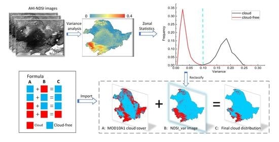
  • The NDSI of each pixel in the 25 AHI images was calculated from 8:30 to 12:30; before that, band2 and band 5 had to be resampled to 500m in order match to MODIS.
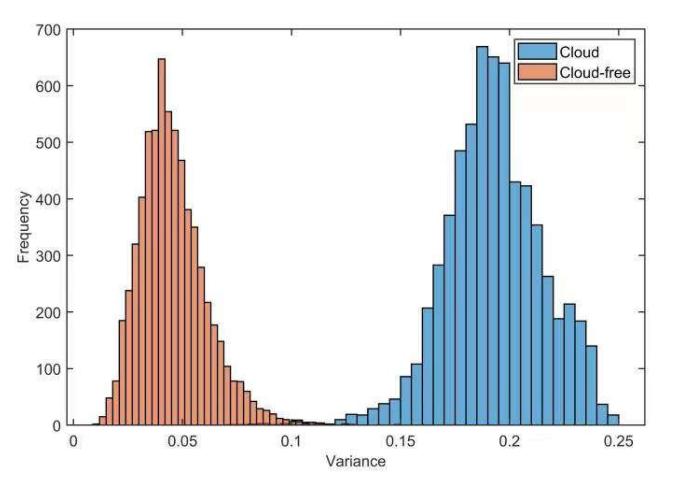
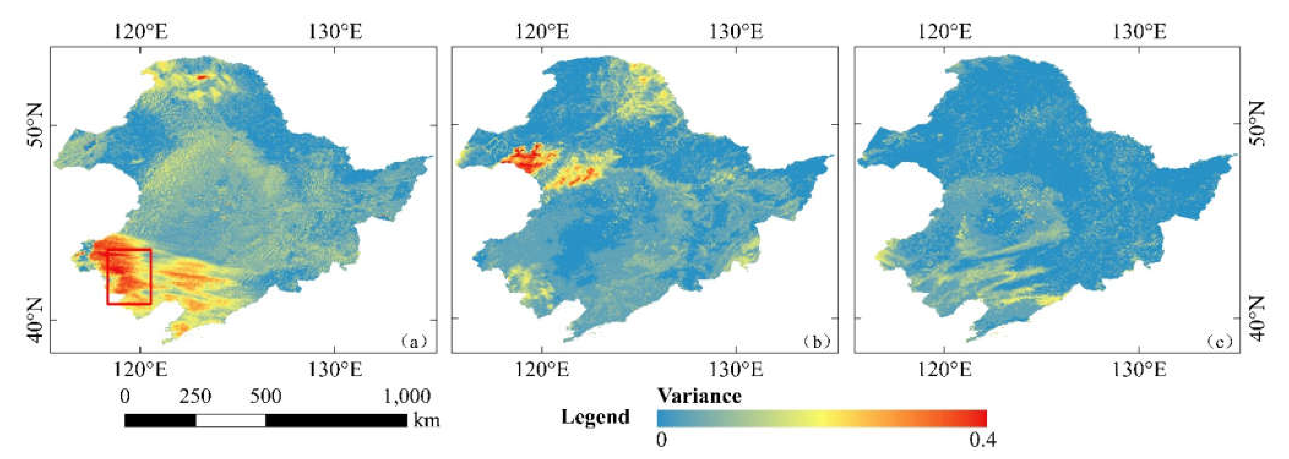
  • The NDSI variance in the AHI images was calculated, and the NDSI variance images were named NDSI_var.
  • For the pixel in NDSI_Snow_Cover with a value of 250, if the corresponding value in NDSI_var was less than 0.1, it was replaced with the raw NDSI of this pixel; otherwise, it was retained as 250. After this step, the pixels that were misclassified as clouds could be restored to their raw NDSI value.
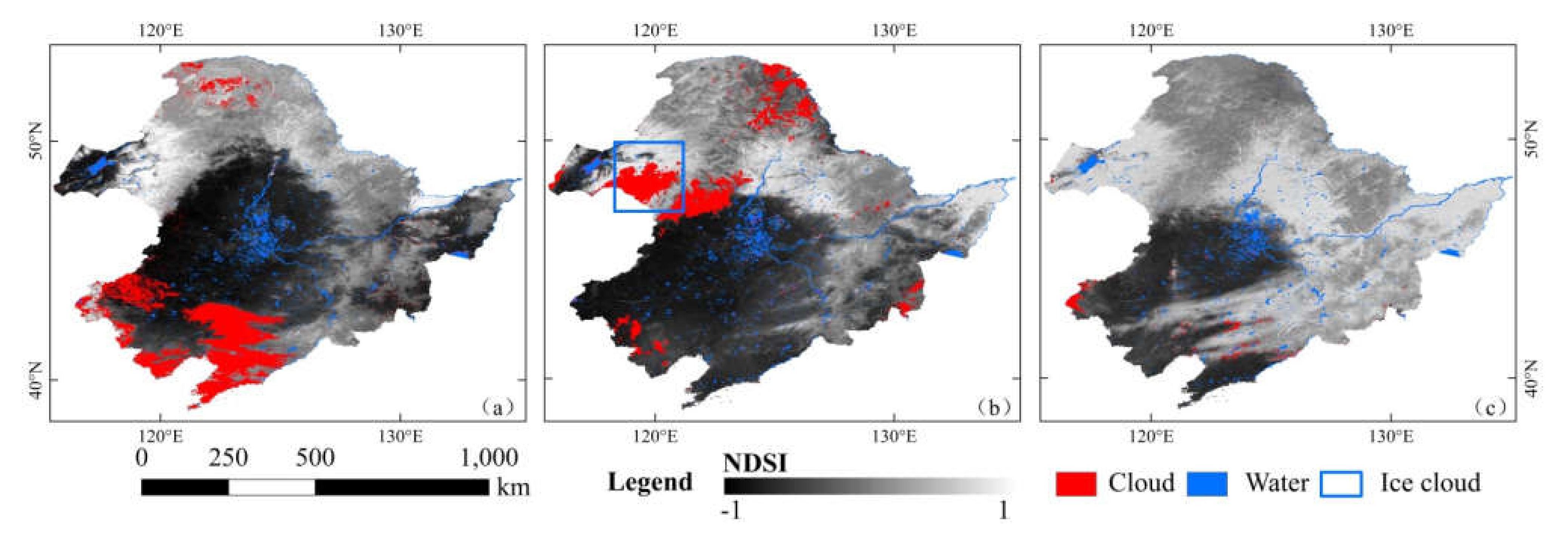
  • For all the pixels in NDSI_Snow_Cover with values greater than 0 and less than 100, if the corresponding value in NDSI_var was equal to or greater than 0.1, then the pixel value was changed to 250. That is, this pixel was thought to probably be an ice cloud. The ice clouds that were misclassified as snow could be identified in this step.

5. Validation and Discussion

5.1. Validation with Example Images

Three MODIS images, acquired on 12 February, 2019, 22 March, 2018, and 16 March, 2018, were used to verify the algorithm. Figure 8a–c shows false-color reflectance images combined with bands 2/4/6, in which snow and clouds (except ice clouds with the same spectral characters as snow) appear in different colors, snow being yellow, and clouds being white. Figure 9a–c shows the cloud distribution in the MOD10A1 NDSI_Snow_Cover data layer of these 3 days, in which the red pixels are clouds. The cloud fractions were 39.2%, 39%, and 21.6%, respectively. The clouds in MOD10A1 NDSI_Snow_Cover (Figure 9) were much more abundant than in the reflectance images (Figure 8). In Figure 8a,b, only a few clouds are shown in the red rectangles, and clouds are almost negligible in Figure 8c. Figure 8d–f shows three Landsat8 OLI false-color images, L1–L3, which were acquired on the same day as those of Figure 8c. In the OLI images with 30 m resolution, it is clear that there are no clouds.
Figure 10a–c are NDSI_var images, in which the high NDSI_var values roughly correspond to the cloud pixels in Figure 8a–c. After performing the cloud–snow identification experiment on NDSI_var images, the new NDSI_ Snow_Cover layers are shown in Figure 11a–c; the red pixels are new cloud masks. The new cloud distribution appeared to be basically consistent with that in the reflectance images (Figure 8a–c). The cloud cover fraction was reduced to 9.68%, 3.6%, and 0.76%, respectively. The excessive cloud mask in the NDSI_ Snow_Cover layer was greatly reduced. To further evaluate this method quantitatively, five regions of interest (ROIs) in each image were selected (as shown in Figure 8a–c); each of them was about 200*200 pixels. For the pixels in the ROIs, the results from this method were compared, pixel by pixel, with the visual interception results, and the confusion matrix is shown in Table 4. The accuracy of this method was 96.5%,97.9%, and 99.8% respectively.

5.2. Discussion

Cloud–snow identification is a challenging problem, and a large number of algorithms have been proposed in recent years [56,57,58]. Many spectral tests cannot distinguish clouds and snow very well and heavily rely on predefined thresholds. Some methods may produce incorrect detection results that misclassify snow as clouds. In MOD10A1 C6, the accuracy of cloud and snow recognition was improved. However, as shown in Figure 8, during the snow season, much snow was misclassified as clouds, especially in forest areas. This finding is consistent with those of previous research [26,27], which found that the cloud mask is very unreliable in winter and is greater than that observed at meteorological stations.
In this paper, we did not perform cloud–snow identification based on the original reflectance data but we used the MODIS snow product MOD10A1 to reduce cloud–snow confusion. We tried to find cloud-free pixels from the pixels that were marked as clouds and pixels that might be clouds from the pixels that were defined as snow; then, we produced a reliable cloud mask.
As shown in Figure 11a–c, most snow marked as clouds in MOD10A1 was recovered. In Figure 10a, some pixels (in the red rectangle box) had high NDSI variance, but they were not clouds according to the false-color image of Figure 8a and they were not marked as clouds in MOD10A1 as shown in Figure 9a. The probable reason is that some clouds passed that area between 8:30 and 12:30 AM but not at 10:30. Because we only identified pixels that were marked as clouds in MOD10A1, these pixels were not modified as clouds in the new NDSI_Snow_Cover of Figure 11a, although they had high NDSI variance. That is, our approach did not introduce redundant clouds.
Most cloud pixels that were reevaluated as cloud-free regions were located in forest areas, such as Daxing’an Mountains, Xiaoxing’an Mountains, and Changbai Mountains. Because of crown obscurity, the mixed pixel of snow and forest crown had a lower NDSI value and a lower visible reflectance than pure snow and therefore were misclassified as clouds. Some other pixels were located in the transition zone between snow and snow-free areas.
Take the image acquired on 16 March 2018 as an example to analyze the NDSI distribution of the snow season in Northeast China. As shown in Figure 12, the white pixels are pixels with NDSI greater than 0.4 in NDSI_Snow_Cover, which is consistent with the snow distribution shown in Figure 8c; that is, pure snow can be recognized in MOD10A1. In Daxing’an Mountains, Xiaoxing’an Mountains, and Changbai Mountain, most of the NDSI values were between 0.1 and 0.4, and some of them were less than 0.1 (the yellow and red pixels in Daxing’an Mountains). In the transition zone from snow to snow-free areas, the NDSI value was increasingly smaller and showed an obvious zonal distribution, as shown in Figure 12. In boreal areas with snow cover, a large amount of forest snow cover was misclassified as clouds due to its low NDSI value, which led to an obvious excessive cloud masking phenomenon in this area; this will increase the difficulty of cloud removal for snow products and reduce the accuracy of cloudless snow products.
In the restored cloud-free pixels, some pixels had NDSI values lower than 0.1 in the forest area on Daxing’an Mountains (yellow pixels). These pixels indicated snow-covered areas according to the Landsat OLI image acquired at the same time. In the NDSI_Snow_Cover data array of MOD10A1 C6, pixels with 0 < NDSI < 0.1 were defined as no snow, and their value was set to 0 according to the low NDSI screen. Therefore, a low NDSI screen will cause the omission of snow in boreal forest areas.
It is difficult to discriminate ice clouds from snow due to their similar spectral characteristics. However, it is feasible to discriminate them according to the difference in pixel stability. In Figure 11b, some likely ice clouds are marked in the blue box. These pixels seem to be snow in the false-color image in Figure 8b and were not marked as clouds in the NDSI_Snow_Cover in Figure 9b. On the one hand, these pixels may be ice clouds because their NDSI variance is high; on the other hand, they may be snow, and the high NDSI variance is caused by clouds passing this region before or after Terra passed. Regardless, we marked them as clouds to avoid possible snow commission errors.

6. Conclusions

MODIS snow product C6 improved the identification of clouds and snow; in addition, a series of screens were adopted to reduce the misclassification of snow, including low-NDSI screens, low-reflectance screens, and low-solar-elevation screens. These screens are significant for global snow production but may result in snow omission errors in high-latitude boreal forest areas. In the snow covering boreal forests and transition zones from snow to snow-free areas, pixels always have a low NDSI and are easily misclassified as clouds. Ice clouds have spectrum characteristics that are similar to those of snow, so it is difficult to distinguish them based only on the traditional SNOMAP algorithm.
The geostationary meteorological satellite has a high temporal resolution, and snow is stable, while clouds are variable in temporal-sequence images. In this paper, the NDSI variance in temporal-series images was used to qualify the stability of a pixel. For all the cloud pixels in MOD10A1, if a cloud pixel with NDSI variance less than the threshold was defined as cloud-free, its raw NDSI value was restored. At the same time, if the snow pixel had a high NDSI variance, it was marked as clouds. The results show that excessive cloud masks can be effectively reduced and that ice clouds can potentially be distinguished from snow with this method. Furthermore, this method is based on the stability of one pixel in a temporal sequence and is not affected by the spatial heterogeneity of the image.

Author Contributions

X.W. and S.C. designed the algorithm; H.G. Data curation; X.W. drafted the manuscript; C.H. and Z.O. drew some of the maps; J.W. and X.H. reviewed and edited the manuscript. All authors have read and agreed to the published version of the manuscript.

Funding

This research received no external funding.

Acknowledgments

This research was funded by the National Natural Science Foundation of China (No. 42125604; 41771373; 42171391).

Conflicts of Interest

The authors declare no conflict of interest.

References

  1. Brown, R.D.; Mote, P.W. The Response of Northern Hemisphere Snow Cover to a Changing Climate. J. Clim. 2009, 22, 2124–2145. [Google Scholar] [CrossRef]
  2. Hall, D.K.; Riggs, G.A. Accuracy assessment of the MODIS snow products. Hydrol. Process. 2007, 21, 1534–1547. [Google Scholar] [CrossRef]
  3. Barnett, T.P.; Adam, J.C.; Lettenmaier, D.P. Potential impacts of a warming climate on water availability in snow-dominated regions. Nature 2005, 438, 303–309. [Google Scholar] [CrossRef] [PubMed]
  4. Alessandri, A.; Catalano, F.; De Felice, M.; Hurk, B.V.D.; Balsamo, G. Varying snow and vegetation signatures of surface-albedo feedback on the Northern Hemisphere land warming. Environ. Res. Lett. 2021, 16, 10. [Google Scholar] [CrossRef]
  5. Thackeray, C.W.; Derksen, C.; Fletcher, C.G.; Hall, A. Snow and Climate: Feedbacks, Drivers, and Indices of Change. Curr. Clim. Change Rep. 2019, 5, 322–333. [Google Scholar] [CrossRef]
  6. Dozier, J.; Painter, T.H. Multispectral and hyperspectral remote sensing of alpine snow properties. Annu. Rev. Earth Planet. Sci. 2004, 32, 465–494. [Google Scholar] [CrossRef] [Green Version]
  7. Immerzeel, W.W.; Droogers, P.; De Jong, S.M.; Bierkens, M.F.P. Large-scale monitoring of snow cover and runoff simulation in Himalayan river basins using remote sensing. Remote Sens. Environ. 2009, 113, 40–49. [Google Scholar] [CrossRef]
  8. Gao, J.; Williams, M.W.; Fu, X.D.; Wang, G.Q.; Gong, T.L. Spatiotemporal distribution of snow in eastern Tibet and the response to climate change. Remote Sens. Environ. 2012, 121, 1–9. [Google Scholar] [CrossRef]
  9. Tang, Z.G.; Wang, J.; Li, H.Y.; Yan, L.L. Spatiotemporal changes of snow cover over the Tibetan plateau based on cloud-removed moderate resolution imaging spectroradiometer fractional snow cover product from 2001 to 2011. J. Appl. Remote Sens. 2013, 7, 14. [Google Scholar] [CrossRef]
  10. Zhang, G.Q.; Xie, H.J.; Yao, T.D.; Liang, T.G.; Kang, S.C. Snow cover dynamics of four lake basins over Tibetan Plateau using time series MODIS data (2001−2010). Water Resour. Res. 2012, 48, W10529. [Google Scholar] [CrossRef]
  11. Huang, X.D.; Deng, J.; Wang, W.; Feng, Q.S.; Liang, T.G. Impact of climate and elevation on snow cover using integrated remote sensing snow products in Tibetan Plateau. Remote Sens. Environ. 2017, 190, 274–288. [Google Scholar] [CrossRef]
  12. Thirel, G.; Salamon, P.; Burek, P.; Kalas, M. Assimilation of MODIS snow cover area data in a distributed hydrological model using the particle filter. Remote Sens. 2013, 5, 5825–5850. [Google Scholar] [CrossRef] [Green Version]
  13. Zhang, F.; Zhang, H.; Hagen, S.C.; Ye, M.; Wang, D.; Gui, D.; Zeng, C.; Tian, L.; Liu, J. Snow cover and runoff modelling in a high mountain catchment with scarce data: Effects of temperature and precipitation parameters. Hydrol. Process. 2015, 29, 52–65. [Google Scholar] [CrossRef]
  14. Zhang, Q.; Xiao, C.X. Cloud detection of rgb color aerial photographs by progressive refinement scheme. IEEE Trans. Geosci. Remote Sens. 2014, 52, 7264–7275. [Google Scholar] [CrossRef] [Green Version]
  15. An, Z.; Shi, Z. Scene learning for cloud detection on remote-sensing images. IEEE J. Sel. Top. Appl. Earth Observ. Remote Sens. 2015, 8, 4206–4222. [Google Scholar] [CrossRef]
  16. Xie, F.Y.; Shi, M.Y.; Shi, Z.W.; Yin, J.H.; Zhao, D.P. Multilevel cloud detection in remote sensing images based on deep learning. IEEE J. Sel. Top. Appl. Earth Observ. Remote Sens. 2017, 10, 3631–3640. [Google Scholar] [CrossRef]
  17. Wu, X.; Shi, Z. Utilizing multilevel features for cloud detection on satellite imagery. Remote Sens. 2018, 10, 1853. [Google Scholar] [CrossRef] [Green Version]
  18. Riggs, G.A.; Hall, D.K.; Román, M.O. MODIS Snow Products User Guide for Collection 6; National Snow and Ice Data Center: Boulder, CO, USA, 2016. [Google Scholar]
  19. Ackerman, S.; Frey, R. MODIS Atmosphere L2 Cloud Mask Product; NASA MODIS Adaptive Processing System; Goddard Space Flight Center: Greenbelt, MD, USA, 2015. [Google Scholar]
  20. Foga, S.; Scaramuzza, P.L.; Guo, S.; Zhu, Z.; Dilley, R.D., Jr.; Beckmann, T. Cloud detection algorithm comparison and validation for operational Landsat data products. Remote Sens. Environ. 2017, 194, 379–390. [Google Scholar] [CrossRef] [Green Version]
  21. Zhu, Z.; Wang, S.; Woodcock, C.E. Improvement and expansion of the Fmask algorithm: Cloud, cloud shadow, and snow detection for Landsats 4–7, 8, and Sentinel 2 images. Remote Sens. Environ. 2015, 159, 269–277. [Google Scholar] [CrossRef]
  22. Ben-Dor, E. A precaution regarding cirrus cloud detection from airborne imaging spectrometer data using the 1.38 um water vapor band. Remote Sens. Environ. 1994, 50, 346–350. [Google Scholar] [CrossRef]
  23. Hall, D.K.; Riggs, G.A.; Salomonson, V.V. Development of Methods for Mapping Global Snow Cover Using Moderate Resolution Imaging Spectroradiometer Data. Remote Sens. Environ. 1995, 54, 127–140. [Google Scholar] [CrossRef]
  24. Stillinger, T.; Roberts Dar, A.; Collar, N.M.; Dozier, J. Cloud Masking for Landsat 8 and MODIS Terra Over Snow-Covered Terrain: Error Analysis and Spectral Similarity Between Snow and Cloud. Water Resour. Res. 2019, 55, 6169–6184. [Google Scholar] [CrossRef] [PubMed] [Green Version]
  25. Cao, Y.; He, Y.J.; Zeng, Y.; Luo, Q.; Gao, T. Correction methods of MODIS cloud product based on ground observation data. J. Remote Sens. 2012, 16, 325–342. [Google Scholar]
  26. Ma, J.J.; Wu, H.; Wang, C.; Zhang, X.; Li, Z.Q.; Wang, X.H. Multiyear satellite and surface observations of cloud fraction over China. J. Geophys. Res.-Atmos. 2014, 119, 7655–7666. [Google Scholar] [CrossRef]
  27. Li, P.F.; Dong, L.M.; Xiao, H.C.; Xu, M.L. A cloud image detection method based on svm vector machine. Neurocomputing 2015, 169, 34–42. [Google Scholar] [CrossRef]
  28. Hollstein, A.; Segl, K.; Guanter, L.; Brell, M.; Enesco, M. Ready-to-use methods for the detection of clouds, cirrus, snow, shadow, water and clear sky pixels in sentinel-2 MSI images. Remote Sens. 2016, 8, 666. [Google Scholar] [CrossRef] [Green Version]
  29. Zhu, Z.; Woodcock, C.E. Object-based cloud and cloud shadow detection in andsat imagery. Remote Sens. Environ. 2012, 118, 83–94. [Google Scholar] [CrossRef]
  30. Selkowitz, D.J.; Forster, R.R. An automated approach for mapping persistent ice and snow cover over high latitude regions. Remote Sens. 2016, 8, 16. [Google Scholar] [CrossRef] [Green Version]
  31. Choi, H.; Bindschadler, R. Cloud detection in Landsat imagery of ice sheets using shadow matching technique and automatic normalized difference snow index threshold value decision. Remote Sens. Environ. 2004, 91, 237–242. [Google Scholar] [CrossRef]
  32. Zhu, Z.; Woodcock, C.E. Automated cloud, cloud shadow, and snow detection in multitemporal Landsat data: An algorithm designed specifically for monitoring land cover change. Remote Sens. Environ. 2014, 152, 217–234. [Google Scholar] [CrossRef]
  33. Wang, X.Y.; Chen, S.Y.; Wang, J. An Adaptive Snow Identification Algorithm in the Forests of Northeast China. IEEE J. Sel. Top. Appl. Earth Obs. Remote Sens. 2020, 13, 5211–5222. [Google Scholar] [CrossRef]
  34. Wang, X.Y.; Wang, J.; Che, T.; Huang, X.D.; Hao, X.H.; Li, H.Y. Snow Cover Mapping for Complex Mountainous Forested Environments Based on a Multi-Index Technique. IEEE J. Sel. Top. Appl. Earth Obs. Remote Sens. 2018, 11, 1433–1441. [Google Scholar] [CrossRef]
  35. Francis, A.; Sidiropoulos, P.; Muller, J.P. CloudFCN: Accurate and robust cloud detection for satellite imagery with deep learning. Remote Sens. 2019, 11, 2312. [Google Scholar] [CrossRef] [Green Version]
  36. Parajka, J.; Blöschl, G. Spatio-temporal combination of MODIS images-Potential for snow cover mapping. Water Resour. Res. 2008, 44, 72–84. [Google Scholar] [CrossRef]
  37. Paudel, K.P.; Andersen, P. Monitoring snow cover variability in an agropastoral area in the Trans Himalayan region of Nepal using MODIS data with improved cloud removal methodology. Remote Sens. Environ. 2011, 115, 1234–1246. [Google Scholar] [CrossRef]
  38. Ronco, P.D.; Michele, C.D. Cloud obstruction and snow cover in Alpine areas from MODIS products. Hydrol. Earth Syst. Sci. 2014, 18, 4579–4600. [Google Scholar] [CrossRef] [Green Version]
  39. Gafurov, A.; Bardossy, A. Cloud removal methodology from MODIS snow cover product. Hydrol. Earth Syst. Sci. 2009, 13, 1361–1373. [Google Scholar] [CrossRef] [Green Version]
  40. Gao, Y.; Xie, H.; Yao, T.; Xue, C. Integrated assessment on multitemporal and multi-sensor combinations for reducing cloud obscuration of MODIS snow cover products of the Pacific Northwest USA. Remote Sens. Environ. 2010, 114, 1662–1675. [Google Scholar] [CrossRef]
  41. Hall, D.K.; Riggs, G.A.; Foster, J.L.; Kumar, S.V. Development and evaluation of a cloud-gap-filled MODIS daily snow-cover product. Remote Sens. Environ. 2010, 114, 496–503. [Google Scholar] [CrossRef] [Green Version]
  42. Gafurov, A.; Vorogushyn, S.; Farinotti, D.; Duethmann, D.; Merkushkin, A.; Merz, B. Snow-cover reconstruction methodology for mountainous regions based on historic in situ observations and recent remote sensing data. Cryosphere 2015, 9, 451–463. [Google Scholar] [CrossRef] [Green Version]
  43. Huang, X.D.; Deng, J.; Ma, X.F.; Wang, Y.L.; Feng, Q.S.; Hao, X.H.; Liang, T.G. Spatiotemporal dynamics of snow cover based on multisource remote sensing data in China. Cryosphere 2016, 10, 2453–2463. [Google Scholar] [CrossRef] [Green Version]
  44. Chen, X.N.; Long, D.; Liang, S.L.; He, L.; Zeng, C.; Hao, X.H.; Hong, Y. Developing a composite daily snow cover extent record over the Tibetan Plateau from 1981 to 2016 using multisource data. Remote Sens. Environ. 2018, 215, 284–299. [Google Scholar] [CrossRef]
  45. Hou, J.L.; Huang, C.L.; Zhang, Y.; Guo, J.F.; Gu, J. Gap-filling of MODIS fractional snow cover products via non-local spatio-temporal filtering based on machine learning techniques. Remote Sens. 2019, 11, 90. [Google Scholar] [CrossRef] [Green Version]
  46. Li, M.Y.; Zhu, X.F.; Li, N.; Pan, Y.Z. Gap-Filling of a MODIS Normalized Difference Snow Index Product Based on the Similar Pixel Selecting Algorithm: A Case Study on the Qinghai-Tibetan Plateau. Remote Sens. 2020, 12, 1077. [Google Scholar] [CrossRef] [Green Version]
  47. Chen, S.Y.; Wang, X.Y.; Guo, H.; Xie, P.Y.; Sirelkhatim, A.M. Spatial and Temporal Adaptive Gap-Filling Method Producing Daily Cloud-Free NDSI Time Series. IEEE J. Sel. Top. Appl. Earth Obs. Remote Sens. 2020, 13, 2251–2263. [Google Scholar] [CrossRef]
  48. Dozier, J.; Painter, T.H.; Rittger, K.; Frew, J.E. Time-space continuity of daily maps of fractional snow cover and albedo from MODIS. Adv. Water Resour. 2008, 31, 1515–1526. [Google Scholar] [CrossRef]
  49. Dong, C.Y.; Menzel, L. Producing cloud-free MODIS snow cover products with conditional probability interpolation and meteorological data. Remote Sens. Environ. 2016, 186, 439–451. [Google Scholar] [CrossRef]
  50. Chen, S.Y.; Wang, X.Y.; Guo, H.; Xie, P.Y.; Wang, J.; Hao, X.H. A Conditional Probability Interpolation Method Based on a Space-Time Cube for MODIS Snow Cover Products Gap Filling. Remote Sens. 2020, 12, 3577. [Google Scholar] [CrossRef]
  51. Li, X.; Cheng, G.D.; Jin, H.J.; Kang, E.; Che, T.; Jin, R.; Wu, L.Z.; Nan, Z.T.; Wang, J.; Shen, Y.P. Cryospheric change in China. Glob. Planet Change 2008, 62, 210–218. [Google Scholar] [CrossRef]
  52. Che, T.; Dai, L.Y.; Zheng, X.M.; Li, X.F.; Zhao, K. Estimation of snow depth from passive microwave brightness temperature data in forest regions of Northeast China. Remote Sens. Environ. 2016, 183, 334–349. [Google Scholar] [CrossRef]
  53. Klein, A.G.; Barnett, A.C. Validation of daily MODIS snow cover maps of the Upper Rio Grande River Basin for the 2000–2001 snow year. Remote Sens. Environ. 2003, 86, 162–176. [Google Scholar] [CrossRef]
  54. Warren, S.G. Optical properties of ice and snow. Adv. Earth Space Sci. 1982, 20, 67–89. [Google Scholar] [CrossRef] [PubMed]
  55. Barahona, D.; Nenes, A. Parameterizing the competition between homogeneous and heterogeneous freezing in ice cloud formation-polydisperse ice nuclei. Atmos. Chem. Phys. 2009, 9, 5933–5948. [Google Scholar] [CrossRef] [Green Version]
  56. Paull, D.J.; Lees, B.G.; Thompson, J.A. An Improved Liberal Cloud-Mask for Addressing Snow/Cloud Confusion with MODIS. Photogramm. Eng. Remote Sens. 2015, 81, 119–129. [Google Scholar] [CrossRef]
  57. Bormann, K.J.; McCabe, M.F.; Evans, J.P. Satellite based observations for seasonal snow cover detection and characterisation in Australia. Remote Sens. Environ. 2012, 123, 57–71. [Google Scholar] [CrossRef]
  58. Sirguey, P.; Mathieua, R.; Arnaud, Y. Subpixel monitoring of the seasonal snow cover with MODIS at 250 m spatial resolution in the Southern Alps of New Zealand: Methodology and accuracy assessment. Remote Sens. Environ. 2009, 113, 160–181. [Google Scholar] [CrossRef]
Figure 1. Land cover map of the study area.
Remotesensing 14 01372 g001
Figure 2. Average number of CCDs per month in Northeast China from 2014 to 2018, counted based on MOD10A1.
Remotesensing 14 01372 g002
Figure 3. Average number of CCDs per month for the three stations from 2014 to 2018, counted based on MOD10A1; (a) station 1, (b) station 2, (c) station 3.
Remotesensing 14 01372 g003
Figure 4. Average cloud coverage every month in Northeast China from 2014 to 2018, determined based on CRU TS4.04.
Remotesensing 14 01372 g004
Figure 5. False-color image of the study area (a) acquired on 10 January, 2018, combined with bands 1/2/4, (b) acquired on 10 January, 2018, combined with bands 2/4/6, (c) acquired on 1 July, 2018, combined with bands 1/2/4, (d) acquired on 1 July, 2018, combined with bands 2/4/6.
Remotesensing 14 01372 g005
Figure 6. Spectral curves of cloud and snow.
Remotesensing 14 01372 g006
Figure 7. NDSI variance in snow and common clouds.
Remotesensing 14 01372 g007
Figure 8. False-color reflectance images of MODIS combined with bands NIR/Green/SWIR and of OLI combined with bands NIR/Red/Green. (a) MODIS acquired on 12 February 2019, (b) MODIS acquired on 22 March 2018, (c) MODIS acquired on 16 March 2018, (d) OLI_L1 acquired on 16 March 2018, (e) OLI_L2 acquired on 16 March, 2018, (f) OLI_L3 acquired on 16 March 2018.
Remotesensing 14 01372 g008
Figure 9. Cloud mask MOD10A1 in the NDSI_Snow_Cover data layer. (a) 12 February, 2019, (b) 22 March, 2018, and (c) 16 March, 2018.
Remotesensing 14 01372 g009
Figure 10. NDSI_var images (a) 12 February 2019, (b) 22 March 2018, and (c) 16 March 2018.
Remotesensing 14 01372 g010
Figure 11. New NDSI_Snow_Cover layer. (a) 12 February 2019, (b) 22 March 2018, and (c) 16 March 2018.
Remotesensing 14 01372 g011
Figure 12. Raw NDSI distribution of images on 16 March 2018.
Remotesensing 14 01372 g012
Table 1. Definition of attributes of NDSI_Snow_Cover in MOD10A1 C6.
CodesDescriptionsCodesDescriptions
0–100NDSI-snow239Ocean
200Missing data250Cloud
201No decision254Detector saturated data
211Night255Fill data
237Inland water
Table 2. Band parameters of MOD09GA.
BandWavelength (um)Resolution (m)
10.620–0.670250
20.841–0.8761250
30.459–0.479500
40.545–0.565500
51.230–1.250500
61.628–1.652500
72.105–2.155500
Table 3. Band parameters of ALI carried on Himawari-8.
BandCentral
Wavelength (um)
Resolution (km)BandCentral
Wavelength (um)
Resolution (km)
10.47196.92
20.511107.32
30.641118.62
40.861129.62
51.621310.42
62.321411.22
73.921512.42
86.221613.32
Table 4. Confusion matrix comparing ground truth and the results of our method.
       Results of Our Method
 12 February 2019 22 March 2018 16 March 2018
cloudsnowcloudsnowcloudsnow
Ground truthcloud40,79935212119114561115232
snow3483152,1972619174,734149198,504
Publisher’s Note: MDPI stays neutral with regard to jurisdictional claims in published maps and institutional affiliations.

