Cotton Cultivated Area Extraction Based on Multi-Feature Combination and CSSDI under Spatial Constraint

Abstract

Cotton is an important economic crop, but large-scale field extraction and estimation can be difficult, particularly in areas where cotton fields are small and discretely distributed. Moreover, cotton and soybean are cultivated together in some areas, further increasing the difficulty of cotton extraction. In this paper, an innovative method for cotton area estimation using Sentinel-2 images, land use status data (LUSD), and field survey data is proposed. Three areas in Hubei province (i.e., Jingzhou, Xiaogan, and Huanggang) were used as research sites to test the performance of the proposed extraction method. First, the Sentinel-2 images were spatially constrained using LUSD categories of irrigated land and dry land. Seven classification schemes were created based on spectral features, vegetation index (VI) features, and texture features, which were then used to generate the SVM classifier. To minimize misclassification between cotton and soybean fields, the cotton and soybean separation index (CSSDI) was introduced based on the red band and red-edge band of Sentinel-2. The configuration combining VI and spectral features yielded the best cotton extraction results, with F1 scores of 86.93%, 80.11%, and 71.58% for Jingzhou, Xiaogan, and Huanggang. When CSSDI was incorporated, the F1 score for Huanggang increased to 79.33%. An alternative approach using LUSD for non-target sample augmentation was also introduced. The method was used for Huangmei county, resulting in an F1 score of 78.69% and an area error of 7.01%. These results demonstrate the potential of the proposed method to extract cotton cultivated areas, particularly in regions with smaller and scattered plots.

1. Introduction

As the world’s largest cotton producer, cotton, as China’s second-largest crop after grain, is a crucial strategic material related to the national economy and people’s livelihood [1,2]. China’s cotton is mainly produced in the Xinjiang province, the Yellow River Basin, and the Yangtze River Basin. Located at the center, Hubei is the most important cotton-producing province in the Yangtze River Basin [3]. Statistical data on cotton cultivated areas is commonly used for cotton yield estimation, economic index monitoring, and agricultural management [4]. Due to changes in regional land use [5] and cotton subsidy policies, coupled with high labor costs due to time-consuming and laborious planting methods, Hubei’s cotton cultivated area has decreased significantly in recent years. However, due to the prevalence of small and fragmented cotton fields, accurately extracting and estimating cotton planting areas have remained extremely challenging, particularly in large areas.

Nowadays, satellite remote sensing technology has been widely used in various agricultural production applications [6,7]. The analysis, collection, processing, and visual display of remote sensing data can be used to classify, extract, and estimate cultivated areas, which is vital in agricultural production management, particularly in growth monitoring, pest control, and yield estimation [8,9,10,11].

A number of studies have employed remote sensing technology and developed various approaches for cotton area extraction and yield estimation. For example, Ahmad et al. [12] combined multi-temporal MODIS data (with a resolution up to 250 m) with Landsat7 TM/ETM+ data (30 m) to extract cotton cultivated area and estimate the yield based on NDVI index, demonstrating the economics and feasibility of large-scale crop yield estimation. With the continuous development of satellite technology, high-resolution satellite image data has been widely used in agricultural production and applications [13,14]. Yi et al. [15] constructed LAI estimation models at different development and growth stages of cotton in northern Xinjiang for various applications, such as cotton yield estimation, growth monitoring, and fertilization monitoring. However, other areas have varying circumstances that make popular RS estimation approaches unsuitable. For example, unlike Xinjiang, which has large and mainly contiguous cotton fields, Hubei’s cotton production comprises smaller and scattered plots. Xu et al. [16] used high spatial resolution satellite images of GF-2 (up to 0.81 m) and QuickBird (up to 0.61 m) for accurate extraction of farmland based on image texture features using object-oriented multi-scale hierarchical partitioning and various local segmentation algorithms. While their approach can accurately extract farmlands in complex landscapes, it is limited by the revisit period and imaging quality of high-resolution satellites. Using an unmanned aerial vehicle (UAV) equipped with a hyperspectral sensor to capture low-altitude images, Liu et al. [17] classified cotton fields by object-oriented segmentation method for yield estimation. However, the cost of acquiring UAV data of large-scale fields is relatively high.

In data processing, algorithms such as deep learning, migration learning, and reinforcement learning are widely used in remote sensing data interpretation, improving the extraction of crop spatial distribution [18,19]. Zhu et al. [20] used deep learning semantic segmentation model for cotton ridge road recognition and utilized improved U-Net networks (i.e., Half-U-Net and Quarter-U-Net), providing a technical basis for the development of cotton field intelligent agricultural machinery navigation equipment. Chen et al. [21] built an improved Faster R-CNN model incorporating dynamic mechanisms to identify the top buds of cotton in the field and verified the feasibility of deep learning image processing algorithms in UAV remote sensing agriculture. Crane-Droesch [22] utilized a semi-parametric variant of a deep neural network to predict annual corn yield in the Midwest of the United States, resulting in better model effect and practical significance than classical statistics and other methods. However, these deep learning-related algorithms have been used mainly in small target areas, and require a large number of sample libraries. These approaches are not suitable for cotton field extraction in areas with limited sample sizes, such as Hubei.

In terms of remote sensing data analysis, time-series images and optimized results can be obtained using various approaches, such as combining auxiliary data (e.g., land-use planning vectors) [23,24], and establishing spatial-temporal data fusion model [25]. Zhang et al. [26] used an SVM extraction algorithm and a cultivated land mask on high-resolution GF series satellite data to differentiate cotton from other crops, considerably improving the efficiency of ground data survey collection. Zhang et al. [27] proposed a new PMI index to monitor the spatial changes in rice, given the difficulties of rice field extraction, particularly during the rice flooding period. A number of studies have also developed field extraction approaches based on vegetation index (VI) from GF-5 AHSI satellite data, using texture features extracted from GF-6 PMS and topographic factors from DEM, and have tested different classification schemes employing Nearest Neighbor, Support Vector Machine, and Random Forest algorithms for regional tree species identification [28,29,30,31]. These studies can be used in developing new extraction approaches for cotton cultivated areas that address the limitations of current methods.

To address the major challenges in RS field extraction for small cultivated plots, this study proposes an innovative remote sensing monitoring approach for cotton cultivated areas at the regional scale using Sentinel-2 images, land use status data (LUSD), and field survey data. The study site is Hubei Province, where cotton plantations are fragmented and irregular, and where cotton and soybean are cultivated together in some areas. Given that the growth cycles of cotton and soybean are similar, cotton extraction can be extremely confusing and highly prone to large errors. We utilized LUSD data as spatial constraint and constructed seven schemes that use spectral features, vegetation index (VI), and texture features. Based on SVM classification algorithm, we incorporated a new cotton and soybean separation difference index (CSSDI) to separate cotton and soybean in adjacent planting plots. For specific areas with few cotton samples, a non-object sample augmentation based on LUSD categories was developed to improve the accuracy of cotton extraction. The results of this study can be used to optimize regional cotton growth monitoring and cultivation management, which are crucial for sustainable agricultural development.

2. Study Area and Data

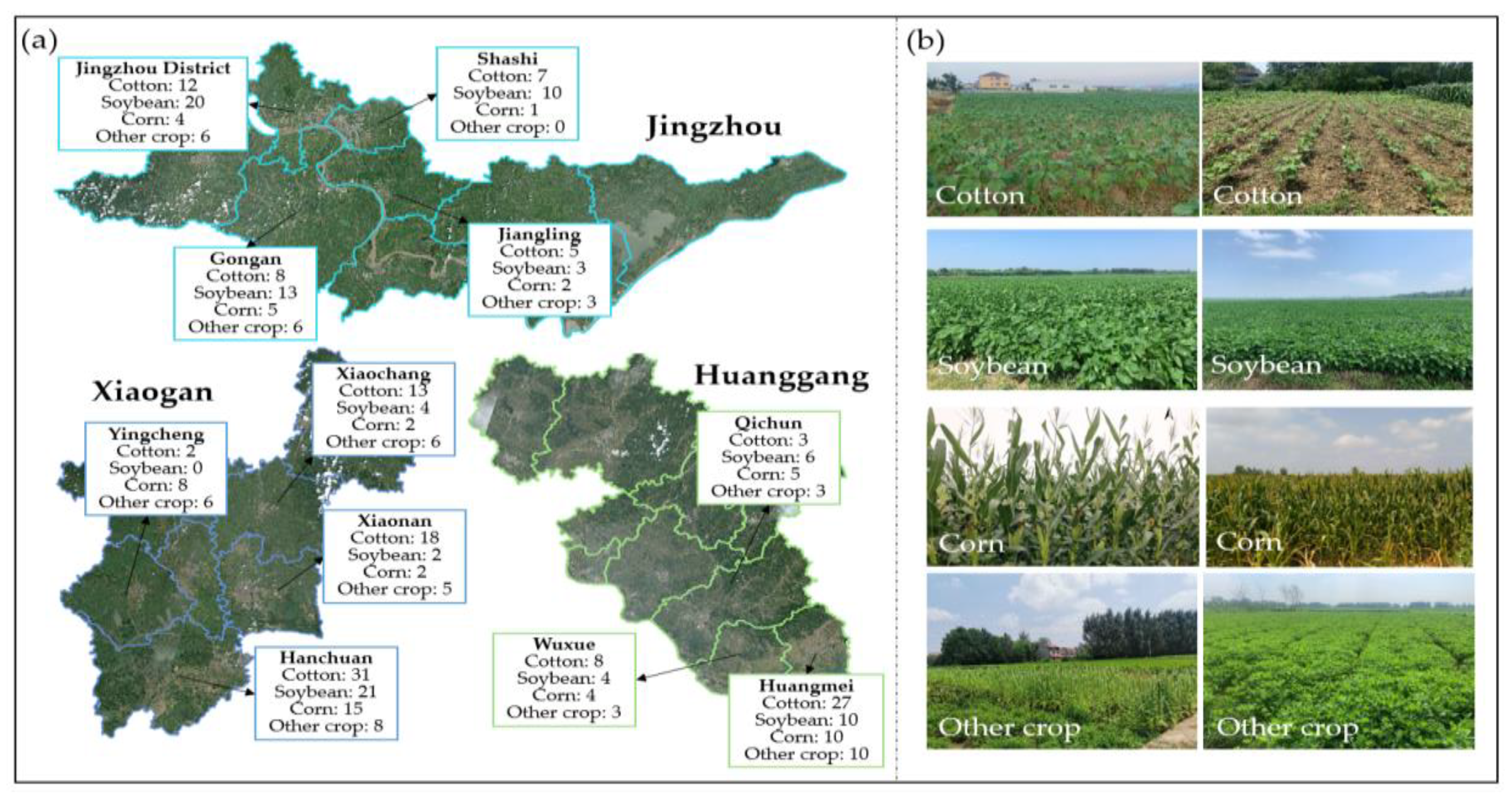
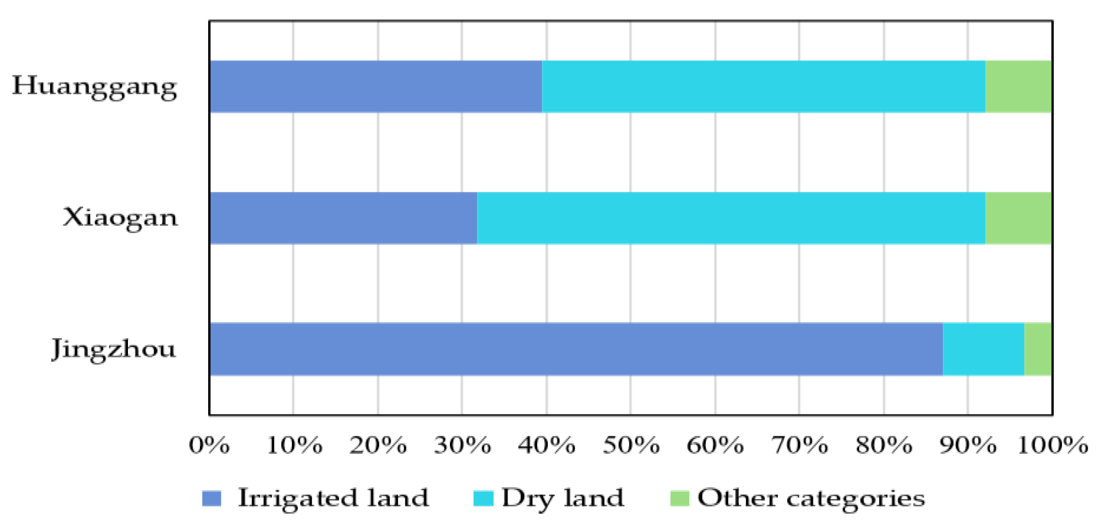
2.1. Study Area

Hubei Province in central China is located between 29°01′53″ N–33°6′47″ N and 108°21′42″ E–116°07′50″ E, with a total area of 185,900 km². Outside its mountainous region, most of the area has a humid subtropical monsoon climate. For this study, three major cotton production areas in Hubei were selected for field sampling and cotton extraction (see Figure 1): Jingzhou, Xiaogan, and Huanggang. These regions have different topography. Jingzhou is mainly composed of plain areas with altitudes ranging from 20–50 m. Xiaogan is mostly hilly, with some mountainous areas in the north and plains in the south. Huanggang is mountainous in the north, with hills and plains in the south.

2.2. Crop Phenology

Cotton is an important economic crop in Hubei. The main growing period is from April to September. After maturity in mid-September, cotton harvesting is carried out in batches, lasting until October. Aside from cotton, the dominant crops in Hubei—rice, corn, and soybean (

Table 1. Percentage of four crops in the total sown area in different regions.

Region	Cotton	Soybean	Rice	Corn
Jingzhou	4.19%	3.84%	42.92%	3.12%
Xiaogan	3.16%	1.54%	72.13%	3.48%
Huanggang	7.42%	3.86%	80.20%	2.72%
Hubei	2.08%	2.71%	29.26%	9.31%

Note: data was from http://tjj.hubei.gov.cn/, accessed on 20 October 2021.

)—share a similar growth period with cotton. In particular, the blooming of cotton, the key stage for feature selection, is highly coincidental with the maturity stage of the soybean, which negatively affects cotton extraction. The phenology information of cotton and other main crops from April to October in Hubei is summarized in

Table 2. The growth cycle of cotton and other crops in Hubei.

Month	Period	Cotton [32,33]	Soybean [34]	Rice [33,35]	Corn [33]
April	Early
	Middle	Sowing
	Late	Seedling		Sowing
May	Early
	Middle			Seedling
	Late	Budding
June	Early		Sowing	Planting	Sowing
	Middle			Tillering
	Late		Maturity		Seedling
July	Early	Blooming		Jointing	Jointing
	Middle
	Late			Heading/ Booting
August	Early				Booting
	Middle				Blooming
	Late			Filling	Filling
September	Early	Harvest
	Middle			Harvest	Harvest
	Late		Harvest
October	Early
	Middle
	Late

Note: Early refers to the first ten days of the month, middle refers to the next ten days, and late refers to the remaining days.

.

2.3. Data

2.3.1. Satellite Data

The satellite images used in this study were Sentinel-2 Level-2A data covering 13 spectral bands, with a temporal resolution of five days and spatial resolutions of 10 m, 20 m, and 60 m. Based on the phenology characteristics of cotton, the images in late August and late September 2020 were selected. The visible red (Band 4), green (Band 3), blue (Band 2), and near-infrared (Band 8) at 10 m resolution were used for crop classification, while the vegetation red-edge bands (Band 5, 6, and 7) at 20 m resolution were used to determine the CSSDI. The pre-processing procedure included band combination, mosaicking, clipping, and cloud masking. The red-edge band images were resampled to 10 m using the nearest neighborhood method. The above steps were carried out in Google Earth Engine.

2.3.2. Land Use Status Data

The land-use status data (LUSD) used in this study were acquired in 2017–2019 from China’s third nationwide land and resources survey. The dataset included information on cultivated land, forest land, residential land, and other primary categories. Each primary category was further decomposed into secondary categories. For instance, cultivated lands were subcategorized into paddy fields, irrigated land, and dry land. In general, cotton, soybean, and corn belong to irrigated or dry land categories, while rice is in the paddy field grouping. LUSD can provide a spatial constraint on the original image, reducing the impact of non-crop and rice on cotton extraction.

2.3.3. Field Sampling Data

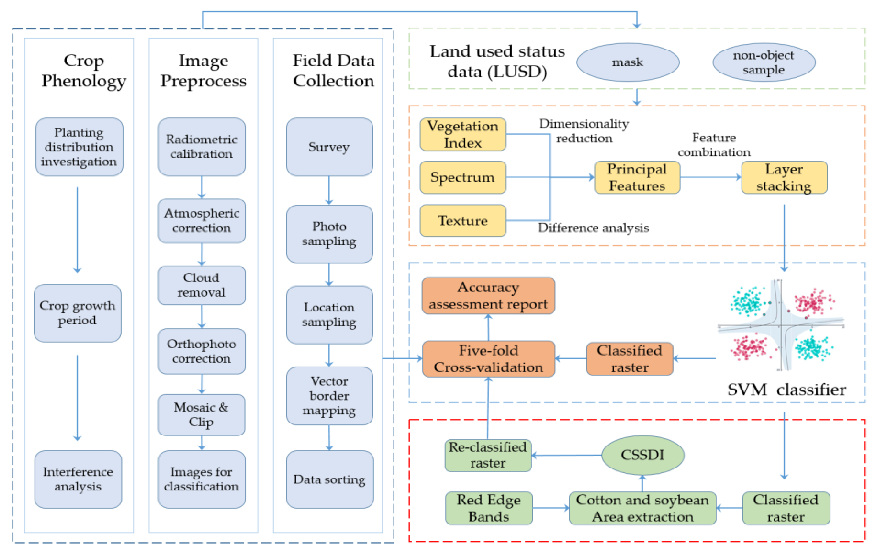
The field survey was conducted during the main growing season for cotton from June to September in Jingzhou, Huanggang, and Xiaogan.. In the field survey, the sampling route was designed using expert knowledge and statistical information from statistical yearbooks and the local Academy of Agricultural Sciences. The station description, including location information, Sentinel and Google Earth Map images, and photos of the sampling points, were obtained for each site.

Table 3. Field sample numbers and areas.

Category	Jingzhou			Xiaogan			Huangang
	No.	Average Area (m2)	Total Area (m2)	No.	Average Area (m2)	Total Area (m2)	No.	Average Area (m2)	Total Area (m2)
Cotton	32	2603	83,310	62	4242	263,028	38	1460	55,496
Soybean	46	2670	122,839	27	4019	108,520	20	4261	85,216
Corn	12	5116	61,392	27	4845	130,812	19	7220	137,176
Other crop	15	5453	81,790	25	6087	152,185	16	5429	86,861

shows the specific sample information, and Figure 2 shows the sampling distribution in Jingzhou, Xiaogan, and Huanggang.

3. Methods

The Sentinel-2 satellite images for Jingzhou, Xiaogan, and Huanggang, acquired in late August and September 2020, were selected for the cotton area extraction. First, pre-processing was performed on the original images, including band combination, mosaicking, clipping, and cloud masking. The pre-processed images were then spatially constrained using the specific categories of LUSD. Another experiment using LUSD was carried out for non-target sample augmentation for cotton extraction in order to make the samples balance for each class and be evenly distributed in each region.

The multi-dimensional features calculated from four bands (i.e., red, green, blue, and near-infrared bands) were selected and combined in seven schemes, which were then used in SVM for crop classification. To have better separation for soybean and cotton fields in Huanggang, CSSDI was established using red-edge and red band.

In order to balance the distribution of training samples and test samples, this study conducted a five-fold cross-validation to test the stability of the proposed model. The technical route of the study is shown in Figure 3.

3.1. Spatial Constraint

In this study, the spatial constraint method was to use the geographic information data, including more detailed plot information and attribute information, to assist satellite images for object classification. According to the technical regulation for category identification of LUSD, cotton is generally divided into irrigated land and dry land. The data was collected in 2019, and the land type may vary for 2019 and 2020. Therefore, this study analyzed the distribution of cotton samples collected in the field in each category of LUSD to verify its reliability.

Figure 4 shows that more than 90% of cotton samples in the three regions belong to the irrigated land and dry land categories, which indicates the reliability of the LUSD. Thus, the Sentinel-2 images were clipped using the irrigated and dry land categories as masks before performing crop classification.

3.2. Feature Selection and Combination

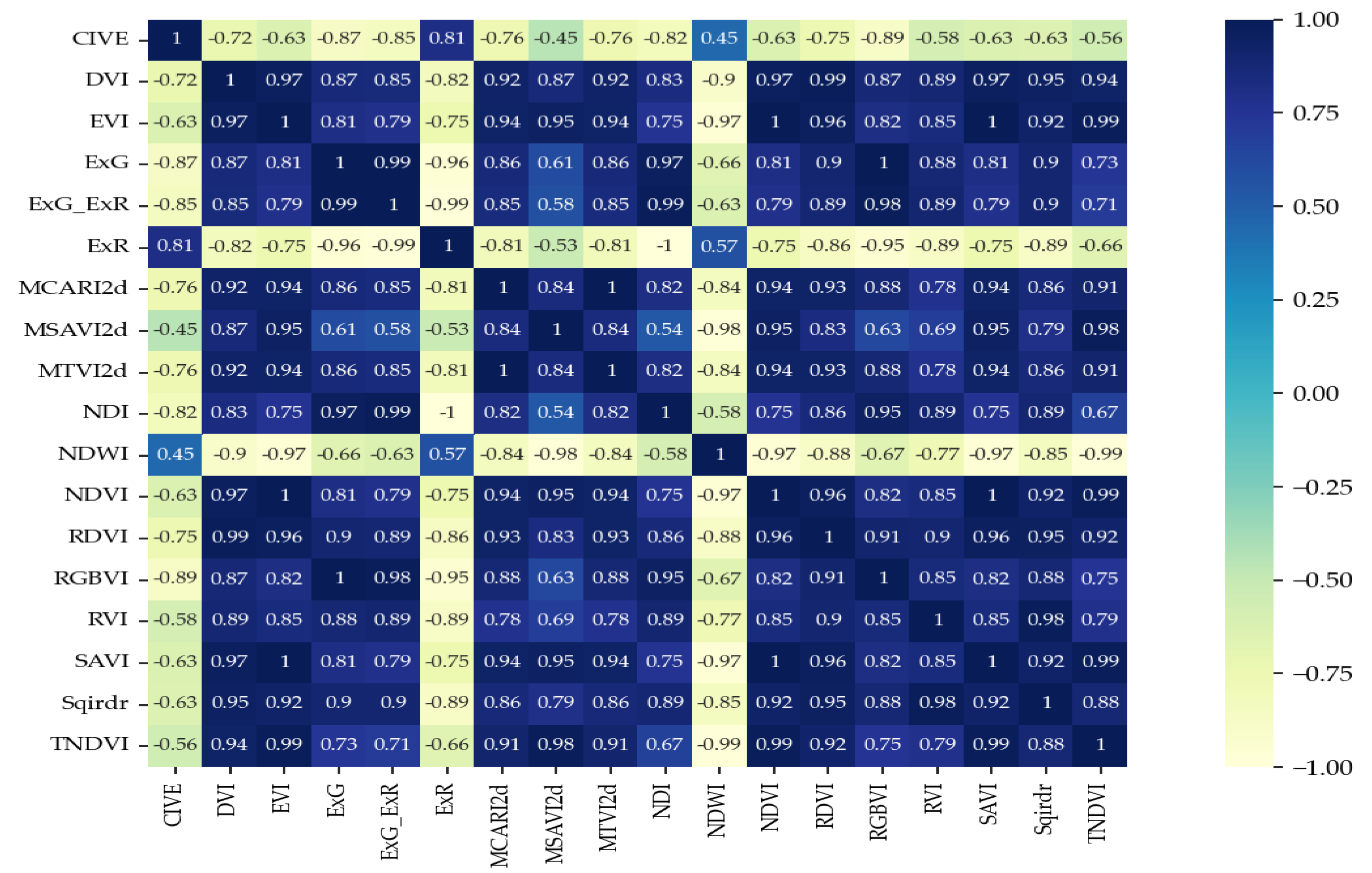
3.2.1. Features Selection

Each Sentinel-2 image has red, green, blue, and near-infrared bands, and all eight spectral bands can be obtained using two-period images. VI is a combination of reflectance of two or more wavelengths to enhance features or details of vegetation. To distinguish the two kinds of features in the paper, we refer to the original bands as spectral features and the band combinations as VI features. In this study, 18 VIs were calculated, and the summary of equations used is presented in Appendix A (

Table A1. Eighteen vegetation indices and their calculation formulas.

No.	Vegetation Index	Abbreviation	Formula	Reference
1	Excess green index	ExG	2 × g − r − b	[45]
2	Excess red index	ExR	1.4 × r − g	[46]
3	Excess green–Excess red	ExG–ExR	ExG − ExR	[46]
4	Color index of vegetation	CIVE	R × 0.441 − g × 0.881 + b × 0.385 + 18.78745	[47]
5	Normalized difference index	NDI	(g − r)/(g + r)	[48]
6	RGB vegetation index	RGBVI	(g2 − b × r)/(g2 + b × r)	[49]
7	Normalized difference vegetation index	NDVI	(nir − r)/(nir + r)	[50]
8	Difference vegetation index	DVI	nir − r	[51]
9	Renormalized difference vegetation index	RDVI	√ (NDVI × DVI)	[52]
10	Ratio vegetation index	RVI	nir/r	[53]
11	Modified chlorophyll absorption in reflectance index	MCARI2d	(((nir − r) × 2.5 − (nir − g) × 1.3) × 1.5)/√((2 × nir + 1) × (2 × nir + 1) − (6 × nir − 5 × √(r)) − 0.5)	[54]
12	Modified Soil Adjusted Vegetation Index	MSAVI2d	(2 × nir + 1−√((2 × nir + 1) × (2 × nir + 1) − 8 × (nir − r))) × 0.5	[55]
13	Modified Triangular Vegetation Index	MTVI2d	((nir − g) × 1.2 − (r − g) × 2.5) × 1.5/√((2 × nir + 1) × (2 × nir + 1) − (6 × nir − 5 × √(r)) − 0.5)	[56]
14	Square root of (IR/R)	SQRT(IR/R)	√(nir/r)	[57]
15	Soil adjusted vegetation index	SAVI	((nir − r) × 1.5)/(nir + r + 0.5)	[58]
16	Transformed normalized difference vegetation index	TNDVI	√((nir − r)/(nir + r) + 0.5)	[59]
17	Enhanced vegetation index	EVI	2.5 × (nir − r)/(nir + 6 × r − 7.5 × b + 1)	[60]
18	Normalized difference water index	NDWI	(g − nir)/(g + nir)	[61]

Note: b, g, r, and nir were the visible blue (Band 2), green (Band 3), red (Band 4), and near-infrared (Band 8) of Sentinel-2, respectively.

). There were strong correlations among some VIs and spectral bands. Therefore, correlation analysis was performed, and features with high correlation were removed to reduce data redundancy. The correlation coefficient threshold was set to 0.9, and VIs and spectral features with more significant differences and small dimensionality were obtained. Figure 5 shows the correlation matrix for the vegetation indices.

Texture features provide supplementary information about object properties and can be helpful for the discrimination of heterogeneous crop fields [36]. In this study, two widely-used texture features for image classification, Entropy and Second Moment [31,37], were used to assist in cotton extraction. To reduce data dimensionality, Principal Component Analysis (PCA) was performed for two Sentinel-2 images, and only the first principal component was used in calculating co-occurrence measures for each texture. The co-occurrence shift included four directions (1, 0), (1, 1), (0, 1), (−1, 1), which represent 0°, 45°, 90°, and 135°, respectively. The results of the co-occurrence shift were averaged, producing the final texture features for Entropy and Second Moment.

3.2.2. Feature Combination

Due to the diversity of crops and the limitation of spectral information acquisition, different objects could be in the same spectrum, and objects in the same category could be in different spectrums. In order to improve cotton extraction accuracy, seven classification schemes were generated according to different combinations of spectral, texture, and VI features selected. The different classification schemes are presented in

Table 4. Classification schemes and number of bands.

No.	Classification Scheme
1	Spectral + Texture + Vegetation index
2	Spectral + Texture
3	Spectral + Vegetation index
4	Texture + Vegetation index
5	Vegetation index
6	Spectral
7	Texture

.

3.3. SVM Algorithm

The SVM classifier provides a powerful supervised classification method [38]. In this study, we selected the radial basis function (RBF) kernel, where the gamma parameter defines the influence of a single training example; a low gamma value means ‘far’, while a high value means ‘near’. After parameter adjustment, the value of gamma was set to 0.1. The penalty parameter C of the error term trades off the correct classification of training examples against the maximization of the decision function margin. For larger values of C, a smaller margin is accepted if the decision function is better at classifying all training points correctly. Lower C encourages a larger margin, which means a simpler decision function at the cost of training accuracy. After exploring, the value of penalty, parameter C was set to 1.0. Four categories were used as input: cotton, soybean, corn, and other crops.

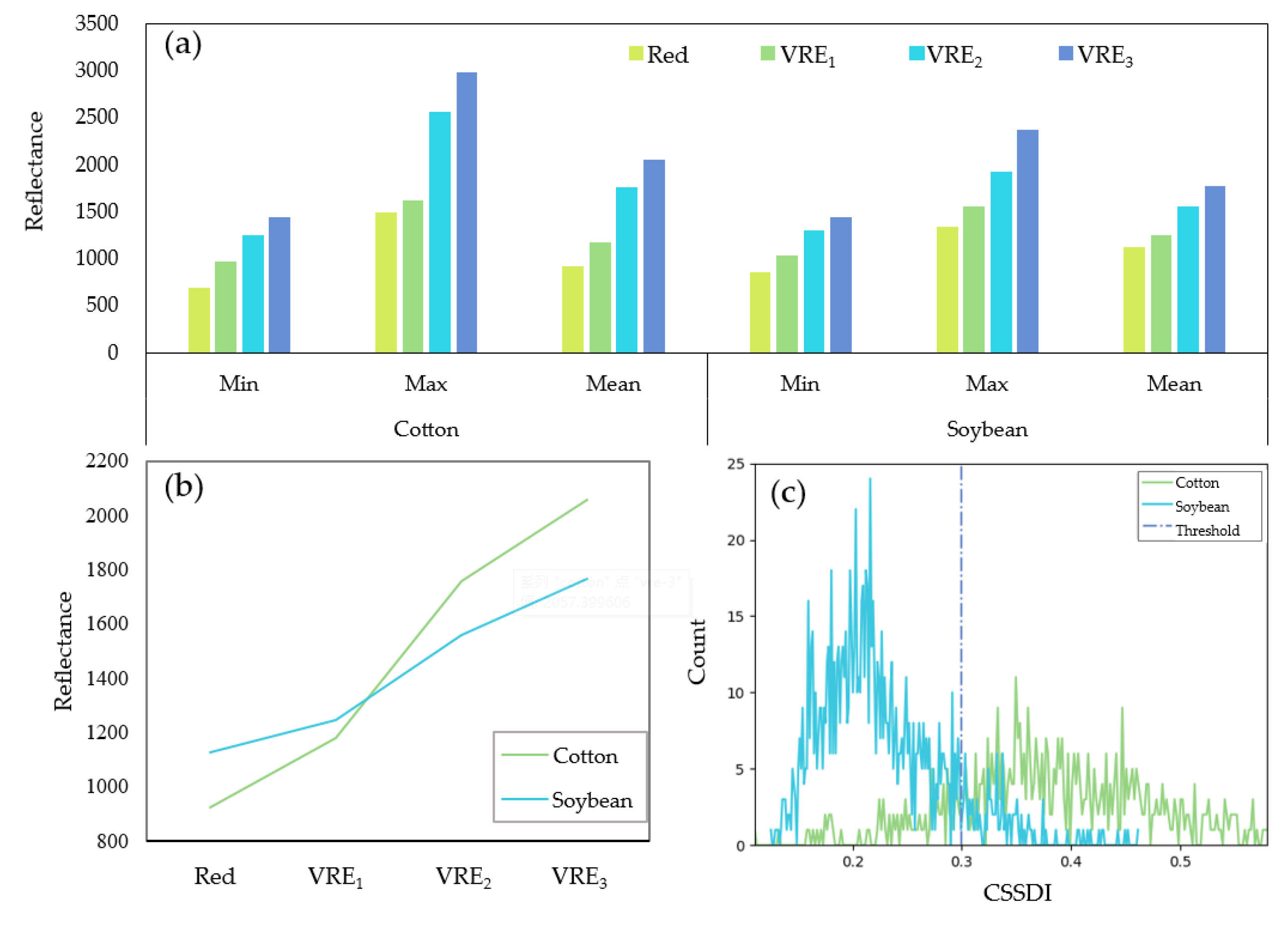
3.4. Cotton and Soybean Separation Difference Index

In some regions of Hubei, particularly in Huanggang, cultivated cotton areas have been changed into soybean fields, resulting in mixed cotton and soybean cultivation. Due to similar growth cycles and similar features in the visible and near-infrared bands, cotton and soybean are difficult to separate using the SVM classifier. The red-edge bands are closely related to the vegetation growth state. Sentinel-2 has vegetation red-edge bands, i.e., Band 5 (VRE₁), Band 6 (VRE₂), and Band 7 (VRE₃), with central wavelengths of 705 nm, 740 nm, and 783 nm, respectively.

This study compared the red band and the three red-edge bands of cotton and soybean. As shown in Figure 6a,b, there were significant differences in the red band and VRE₃ between cotton and soybean. Therefore, an index was developed based on the red band and VRE₃ in Sentinel-2 to differentiate between cotton and soybean. The index, termed the cotton and soybean separation difference index (CSSDI), is calculated using the formula:

$$CSSDI=\frac{VR{E}_3+Red}{VR{E}_3-Red}$$

(1)

where VRE₃ and Red were Band 7 and Band 4 of Sentinel-2.

After calculating the CSSDI, the t-test for cotton and soybean was performed. The resulting p-value was less than 0.01, indicating that there is a significant difference in CSSDI values for cotton and soybean. The CSSDI and pixel count values for cotton and soybean were plotted to define the separation threshold (see Figure 6c). The minimum overlapping values of CSSDI ranged from 0.275 to 0.344. An increment value of 0.003 was applied from the lower limit of 0.275 to the upper limit of 0.344. The accuracy was calculated for each threshold value to find the optimal threshold value for segmentation. The final threshold of 0.299 gave the maximum separation level and highest accuracy.

3.5. Evaluation Index

The field samples were divided into a training set and a test set at a 4:1 ratio, and a five-fold cross-validation was conducted. A confusion matrix was established, and the accuracy of the crop classification model was assessed in terms of overall accuracy (OA) and Kappa coefficient. Producer’s accuracy, user’s accuracy, and F1 score (F1) were used to assess the results of the cotton area extraction. F1 is the harmonic producer’s accuracy and user’s accuracy.

Another evaluation index for cotton extraction is area error (Equation (2)), calculated using the formula:

$$Area error=\frac{abs\left(A_{image}-A_{\mathrm{statistics}}\right)}{A_{\mathrm{statistics}}}\times 100\%$$

(2)

where $A_{image}$ is the extracted cotton cultivated area and $A_{image}$ and $A_{\mathrm{statistics}}$ are the actual cotton cultivated area. The data used for calculating the area error was the 2020 dataset for Jingzhou, Xiaogan, and Huanggang obtained from official government statistics (http://tjj.hubei.gov.cn/tjsj/, accessed on 20 October 2021).

4. Results

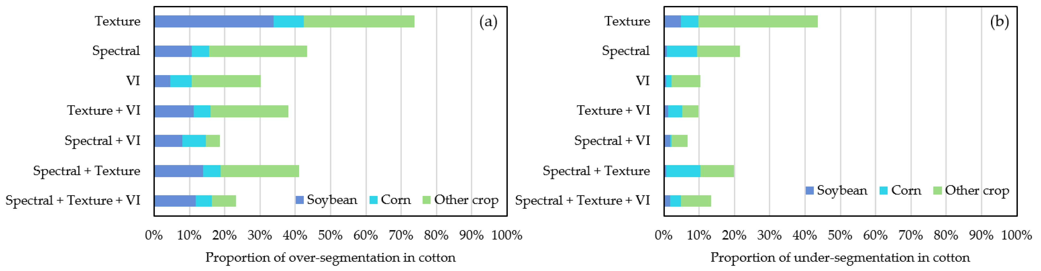
4.1. Classification Result of Feature Combination for Cotton Extraction

Figure 7 shows the results of feature selection, which includes one spectral feature (green band), one VI (RVI), and two texture features (Entropy and Second Moment) for the August image, and one spectral feature (near-infrared band) and three VIs (NDVI, MCARI2d, and RGBVI) for the September image. By the end of August, since cotton is in the blooming stage, it exhibits its typical feature. At the end of September, cotton and other crops with similar growth cycles are in harvest. However, the cotton harvest is carried out in batches and lasts until October, which can show different features in images compared to other crops.

The three kinds of features were combined into seven classification schemes. The results for the cotton extraction using the SVM classifier are shown in Figure 8. Among the different schemes, the F1 values of the Spectral + VI configuration were highest in the three regions at 86.93%, 80.11%, and 71.58%, respectively. The producer’s accuracy for cotton was greater than the user’s accuracy by 12–17%. This suggests that the errors in the cotton area extraction were mainly due to the misclassification of other crops to cotton. In addition, the three evaluation indices for Jingzhou were higher than for Xiaogan and Huanggang, primarily caused by Jingzhou’s flat terrain, uniform planting patterns, and a consistent growth cycle for cotton. The confusion matrices of optimal results in three regions are listed in Appendix B (

Table A2. F1 results of five-fold cross-validation.

	Jingzhou	Xiaogan	Huanggang (without CSSDI)	Huanggang (with CSSDI)
1	87.15%	78.76%	70.97%	78.69%
2	87.43%	79.46%	71.13%	75.46%
3	85.07%	84.99%	71.18%	79.12%
4	87.04%	75.21%	77.57%	81.26%
5	87.96%	82.13%	66.03%	82.11%
Average F1	86.93%	80.11%	71.58%	79.33%

,

Table A3. Confusion matrix of Spectral + VI in Jingzhou.

		Reference Data (Pixel)
		Cotton	Soybean	Corn	Other Crop	Total
Classified data (pixel)	Cotton	156	11	20	3	190
	Soybean	3	173	8	41	225
	Corn	1	36	81	7	125
	Other crop	8	35	18	113	174
	Total	168	255	127	164	714

,

Table A4. Confusion matrix of Spectral + VI in Xiaogan.

		Reference Data (Pixel)
		Cotton	Soybean	Corn	Other Crop	Total
Classified data (pixel)	Cotton	469	45	57	94	665
	Soybean	19	108	9	16	152
	Corn	27	34	182	27	270
	Other crop	11	29	14	168	222
	Total	526	216	262	305	1309

,

Table A5. Confusion matrix of Spectral + VI in Huanggang without CSSDI.

		Reference Data (Pixel)
		Cotton	Soybean	Corn	Other Crop	Total
Classified data (pixel)	Cotton	88	46	1	2	137
	Soybean	20	124	0	0	144
	Corn	0	0	251	89	340
	Other crop	3	0	22	83	108
	Total	111	170	274	174	729

and

Table A6. Confusion matrix of Spectral + VI in Huanggang using CSSDI.

		Reference Data (Pixel)
		Cotton	Soybean	Corn	Other Crop	Total
Classified data (pixel)	Cotton	96	36	1	0	133
	Soybean	12	134	0	2	148
	Corn	0	0	251	89	340
	Other crop	3	0	22	83	108
	Total	111	170	274	174	729

).

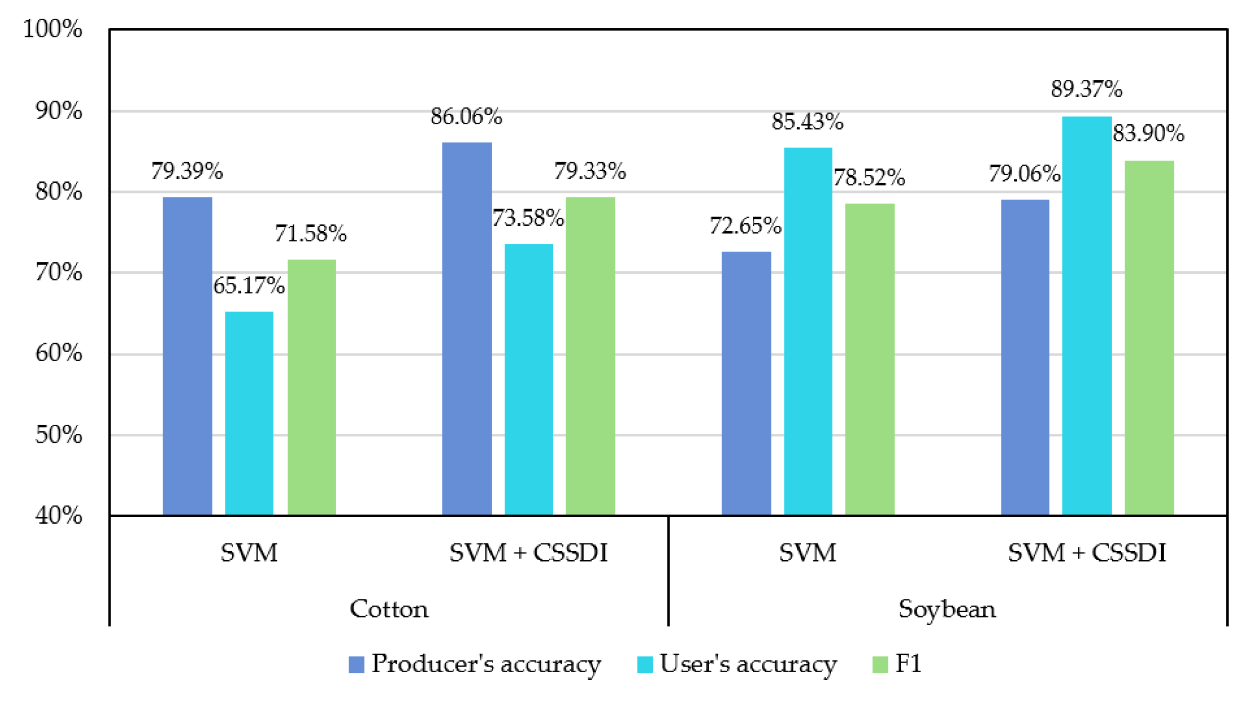
4.2. Improved Results of Cotton Extraction Based on CSSDI

As shown in Figure 8, the three evaluation indices for Huanggang were much lower than for the other two regions, mainly because of misclassification between cotton and soybean. This study proposed a CSSDI based on red and red-edge bands to improve the classification results by further separating cotton and soybean. In Appendix C (Figure A1), different characteristics in the images of the same field can be found, leading to serious misclassification between cotton fields and soybean fields. As shown in Figure 9, the introduction of CSSDI improved the accuracy of cotton area extraction. Producer’s accuracy, user’s accuracy, and F1 increased by 6.67%, 8.41%, and 7.75%, respectively, and the final value of F1 was 79.33%. Similarly, CSSDI also improved the accuracy of soybean extraction. For Xiaogan and Jingzhou, since there were fewer mixed planted areas, the introduction of CSSDI resulted only in marginal improvements in cotton area extraction.

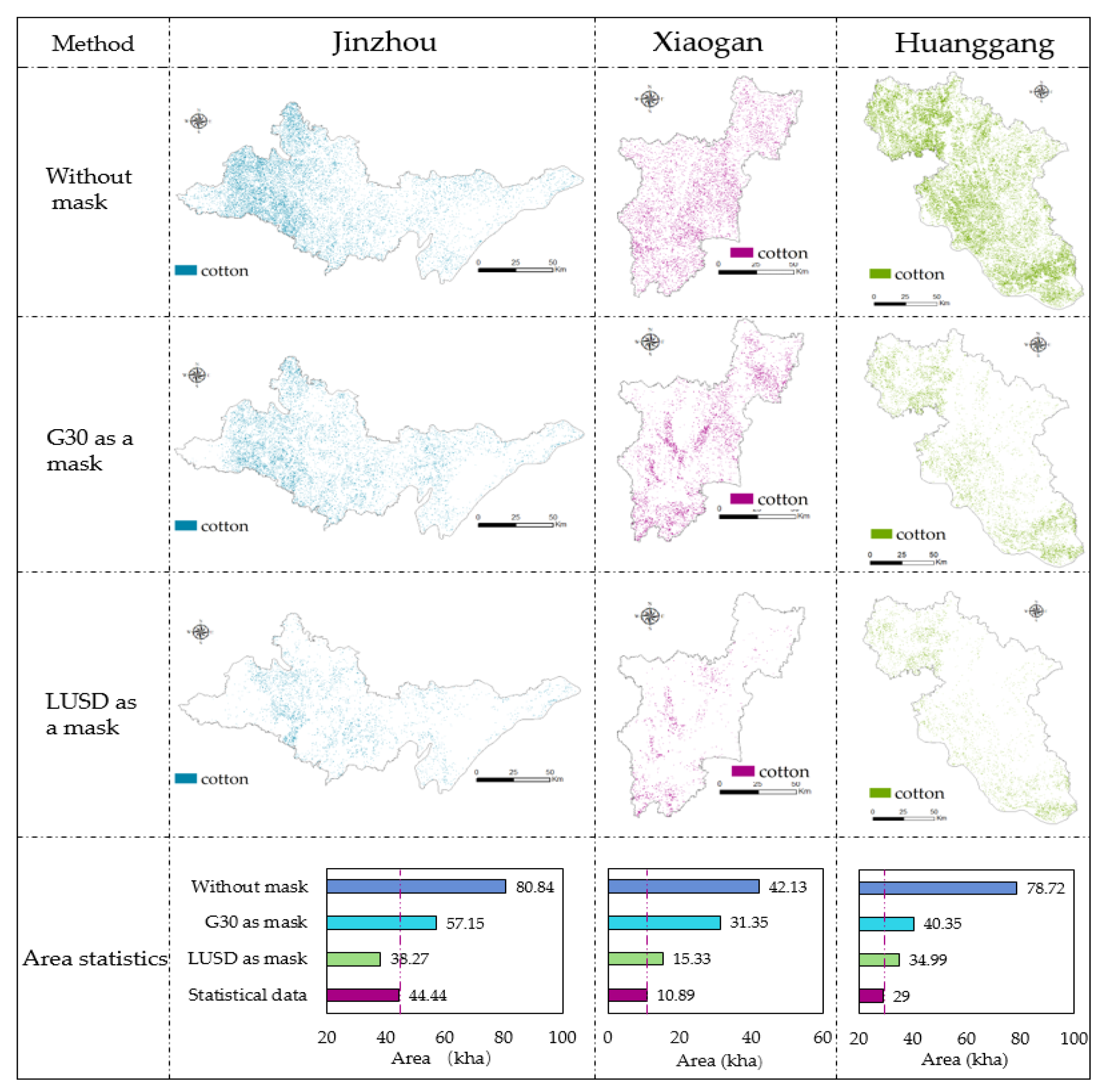
4.3. Comparison of Different Spatial Constraint Methods

To further investigate the performance and explore the advantage of spatial constraint using LUSD, we used two other cotton extraction methods for comparison: (1) without mask and (2) using Globeland30 (G30) data as mask. G30 data provides a global geo-information product available online (http://www.globallandcover.com/, accessed on 10 September 2021). The cultivated land categories of G30 were used as a mask before classification. Aside from cotton, soybean, and corn, the SVM classifier includes a category for rice, which was also collected in the field. For the method without mask, three additional classes were added using visual interpretation to avoid misclassification of non-crops: water, building, and forest.

The cotton extraction accuracy of the three methods was evaluated in two aspects, actual samples collected in the field and actual cotton area from statistical data. The cotton extraction results of the three methods were shown in Figure 10. The concentration of cotton cultivated areas was similar for the three methods. However, the method without mask produced a much larger cotton area compared to the statistical data. This suggests that masking can significantly reduce extracted areas. The LUSD method was closest to the statistical data, with area errors at 13.89%, 40.77%, and 20.66%. Accuracy assessment using samples collected in the field was also performed, and the summary of results is presented in

Table 5. Accuracy evaluation of three methods using field samples.

Method	Evaluation Index	Jingzhou	Xiaogan	Huanggang
Without mask	Producer’s accuracy	93.29%	81.22%	85.45%
	User’s accuracy	75.18%	75.68%	76.50%
	F1	83.26%	78.35%	80.73%
	OA	85.31%	86.03%	95.34%
	kappa	0.82	0.85	0.94
	Area error	81.91%	286.87%	171.45%
G30 as a mask	Producer’s accuracy	85.98%	80.38%	67.67%
	User’s accuracy	74.80%	41.72%	69.12%
	F1	80.00%	54.93%	68.39%
	OA	80.14%	51.65%	74.16%
	kappa	0.75	0.37	0.63
	Area error	28.60%	187.88%	39.14%
LUSD as a mask	Producer’s accuracy	93.29%	85.87%	86.06%
	User’s accuracy	81.38%	76.35%	73.58%
	F1	86.93%	80.83%	79.33%
	OA	72.05%	73.02%	75.25%
	kappa	0.60	0.61	0.65
	Area error	13.89%	40.77%	20.66%

. The LUSD approach produced higher F1 scores than the G30 method, especially in Xiaogan. While the maskless approach generated the highest OA values, the LUSD method can provide a balance between the two evaluation indices of actual area and actual samples.

5. Discussion

5.1. Necessity of Feature Selection and Combination

The performance of different cotton extraction schemes with varying multi-feature combinations was analyzed in this study. As shown in Figure 11, cotton extraction schemes using a single texture feature or spectral feature can result in more over-segmentation or under-segmentation. Schemes with VI features can effectively reduce the misclassification between cotton and corn (Figure 11b), achieving relatively high accuracy of cotton extraction. Although VIs are based on multiple spectral band calculations, the green and near-infrared spectral bands can generate different crop information from VI features. The results suggest that the spectral + VI scheme provides higher accuracy than methods using only a single VI feature.

However, texture features had a relatively smaller role in cotton extraction. Texture features indicate the distribution function statistics of the local crop properties in the image, while spectral and VI reflect the crop-based features of pixels. In this study, the small plot size and coarse spatial resolution of the Sentinel image limited the extraction of representative texture features, causing the texture-feature-based methods to have lower accuracy than spectral + VI. Some studies have also introduced texture features to help crop classification. Using a 2 m spatial resolution WorldView-2 imagery, Wan et al. [39] found that texture and spectral features can slightly improve crop classification compared to using spectral bands alone. Kwak et al. [37] explored the impact of texture information on crop classification based on UAV images with much finer resolution. They concluded that GLCM-based texture features obtain the most accurate classification. These studies suggest the usefulness of texture features for crop classification in high-resolution images. In this study, the combination of features was found to increase crop classification accuracy.

5.2. Advantages of CSSDI for Separating the Cotton and Soybean

To improve crop differentiation and field extraction, we compared the spectral characteristics between cotton and soybean. The biggest spectral differences between the two crops were found in the red-edge band and the red band (Figure 6). Therefore, a new vegetation index CSSDI was proposed. In Huanggang, the F1 scores increased by 7.75%. Red-edge is the spectral feature corresponding to the maximum slope in the reflectance profile of green vegetation [36]. Several studies that evaluated the capabilities of Sentinel-2 for vegetation classification have concluded that the red-edge band contributes significantly to accurate crop classification [40,41]. Xiao et al. developed red-edge indices (RESI) by normalizing three red-edge bands in Sentinel-2, applying them to map rubber plantations [42]. The index was sensitive to changes in moisture content and canopy density of rubber plantations, with an overall accuracy of 92.50% and a kappa coefficient of 0.91. Kang et al. combined NDVI time series and NDRE red-edge time series and used a Random Forest algorithm for crop classification [43], resulting in better crop classification than single NDVI time series.

Due to limitations in spatial resolution, the use of red-edge bands for crop classification would be difficult for the entire Huanggang area. However, the results of this study suggest that red edge bands play a key role in the further separation of soybean and cotton cultivated areas, and that combining the visible, near-infrared, and red-edge bands would result in better cotton area extraction.

5.3. Balance between F1 Scores and Area Errors Using LUSD

The spatial constraint method with LUSD generated high F1 scores in Jingzhou, resulting in comparable area estimates with the statistical data. For Huanggang and Xiaogan, the cotton area estimates were 21–41% higher than the statistical data, which means that other categories were misclassified as cotton.

The Huangmei county with more area error was selected as the test area. A non-object sample augmentation was performed based on LUSD categories (e.g., water, building, forest, shrub, and bare land), and the LUSD samples were evenly distributed throughout the study area. The classes of cotton and other crops used samples collected in the field. The classification results are shown in Figure 12. Although the F1 score of the sample augmentation method was slightly lower than that of the mask method, the cotton area estimate was closer to the statistical values, with a difference of 0.49 kha (see

Table 6. Accuracy evaluation of cotton extraction in Huangmei county using LUSD as a mask or data augmentation.

Evaluation Index	LUSD for Mask	LUSD for Sample Augmentation
Producer’s accuracy	86.43%	80.80%
User’s accuracy	73.19%	76.68%
F1	79.26%	78.69%
OA	75.58%	83.80%
kappa	0.65	0.80
Area error	58.51%	7.01%

). The SVM algorithm created a serious salt-and-pepper phenomenon in the segmentation images, especially at the object boundaries [44]. The small number of sample types resulted in more noise in the cotton category. Although post-processing of classified images by morphological methods can reduce noise, these were not suitable for this study due to the small size of cotton plots in the research area, which may be regarded as noise. Therefore, given the small cotton field and limited samples available in this study, the sample types can be increased using LUSD to reduce the pixels of cotton misclassification to ensure the F1 scores of the cotton and reduce the area errors compared with statistical data.

6. Conclusions

This study used the spatial constraint method and a multi-feature combination based on the SVM algorithm to extract cotton-cultivated areas in Hubei. The present work demonstrates a promising method for cotton extraction for areas with small plots and limited field samples. In this paper, the main contributions are as follows:

1. Through the establishment of seven kinds of feature combination schemes, the optimal scheme was selected for cotton extraction;

2. Further, the CSSDI was established to improve the extraction accuracy of cotton, considering the phenomenon of cotton and soybean mixture;

3. Using LUSD for spatial constraints in this study serves two purposes: (a) LUSD can provide accurate land type information to reduce the influence of non-crop on cotton; (b) non-object sample augmentation is carried out to solve the problem of a small sample number.

For the multi-feature combination, the scheme with VI and spectral features produced the optimal extraction accuracy, with F1 scores of 86.93%, 80.11%, and 71.58% for Jingzhou, Xiaogan, and Huanggang. In addition, the CSSDI was used to further differentiate cotton and soybean, increasing the F1 score in Huanggang to 79.33%. The spatial constraint method using LUSD can effectively reduce area errors for cotton extraction. The relative error for the cotton areas in Jingzhou was 13.89%; however, there were relatively more area errors in the other two regions. An alternative approach (i.e., non-object sample augmentation) was discussed for Huangmei county, and the area error was from 58.51% to 7.01%.

The CSSDI proposed in this paper is only for mixed planting of cotton and soybean in Huanggang. However, in the field investigation, we found mixed planting of cotton with other crops (e.g., watermelon, sesame, and peanut). Therefore, other index model sets need to be constructed in the next stage of research. Moreover, in the follow-up study, we will consider adding auxiliary data with social attribute information to further synthesize the cotton area extraction method. At the same time, we will collect more samples and optimize the feature combination strategy to improve the model and achieve higher crop classification accuracy.

References

1. Ren, Y.; Meng, Y.; Huang, W.; Ye, H.; Han, Y.; Kong, W.; Zhou, X.; Cui, B.; Xing, N.; Guo, A.; et al. Novel vegetation indices for cotton boll opening status estimation using Sentinel-2 data. Remote Sens. 2020, 12, 1712. [Google Scholar] [CrossRef]
2. Mao, H.; Meng, J.; Ji, F.; Zhang, Q.; Fang, H. Comparison of machine learning regression algorithms for cotton leaf area index retrieval using Sentinel-2 spectral bands. Appl. Sci. 2019, 9, 1459. [Google Scholar] [CrossRef] [Green Version]
3. Lu, X.; Jia, X.; Niu, J. The present situation and prospects of cotton industry development in China. Sci. Agric. Sin. 2018, 51, 26–36. [Google Scholar]
4. Xun, L.; Zhang, J.; Cao, D.; Yang, S.; Yao, F. A novel cotton mapping index combining Sentinel-1 SAR and Sentinel-2 multispectral imagery. ISPRS J. Photogramm. Remote Sens. 2021, 181, 148–166. [Google Scholar] [CrossRef]
5. Yohannes, H.; Soromessa, T.; Argaw, M.; Dewan, A. Impact of landscape pattern changes on hydrological ecosystem services in the Beressa watershed of the Blue Nile Basin in Ethiopia. Sci. Total Environ. 2021, 793, 148559. [Google Scholar] [CrossRef] [PubMed]
6. Huang, Y.; Chen, Z.; Tao, Y.; Huang, X.; Gu, X. Agricultural remote sensing big data: Management and applications. J. Integr. Agric. 2018, 17, 1915–1931. [Google Scholar] [CrossRef]
7. Chlingaryan, A.; Sukkarieh, S.; Whelan, B. Machine learning approaches for crop yield prediction and nitrogen status estimation in precision agriculture: A review. Comput. Electron. Agric. 2018, 151, 61–69. [Google Scholar] [CrossRef]
8. Wang, N.; Zhai, Y.; Zhang, L. Automatic cotton mapping using time series of Sentinel-2 images. Remote Sens. 2021, 13, 1355. [Google Scholar] [CrossRef]
9. Chaves, M.E.D.; de Carvalho Alves, M.; De Oliveira, M.S.; Sáfadi, T. A geostatistical approach for modeling soybean crop area and yield based on census and remote sensing data. Remote Sens. 2018, 10, 680. [Google Scholar] [CrossRef] [Green Version]
10. Yang, L.; Wang, L.; Huang, J.; Mansaray, L.R.; Mijiti, R. Monitoring policy-driven crop area adjustments in northeast China using Landsat-8 imagery. Int. J. Appl. Earth Obs. Geoinf. 2019, 82, 101892. [Google Scholar] [CrossRef]
11. Li, X.-Y.; Li, X.; Fan, Z.; Mi, L.; Kandakji, T.; Song, Z.; Li, D.; Song, X.-P. Civil war hinders crop production and threatens food security in Syria. Nat. Food 2022, 3, 38–46. [Google Scholar] [CrossRef]
12. Ahmad, F.; Shafique, K.; Ahmad, S.R.; Ur-Rehman, S.; Rao, M. The utilization of MODIS and landsat TM/ETM+ for cotton fractional yield estimation in Burewala. Glob. J. Hum. Soc. Sci. 2013, 13, 7. [Google Scholar]
13. Stoian, A.; Poulain, V.; Inglada, J.; Poughon, V.; Derksen, D. Land cover maps production with high resolution satellite image time series and convolutional neural networks: Adaptations and limits for operational systems. Remote Sens. 2019, 11, 1986. [Google Scholar] [CrossRef] [Green Version]
14. Jia, X.; Wang, M.; Khandelwal, A.; Karpatne, A.; Kumar, V. Recurrent Generative Networks for Multi-Resolution Satellite Data: An Application in Cropland Monitoring. In Proceedings of the 28th International Joint Conference on Artificial Intelligence, Macao, China, 10–16 August 2019. [Google Scholar]
15. Yi, Q. Remote estimation of cotton LAI using Sentinel-2 multispectral data. Trans. CSAE 2019, 35, 189–197. [Google Scholar]
16. Xu, L.; Ming, D.; Zhou, W.; Bao, H.; Chen, Y.; Ling, X. Farmland extraction from high spatial resolution remote sensing images based on stratified scale pre-estimation. Remote Sens. 2019, 11, 108. [Google Scholar] [CrossRef] [Green Version]
17. Liu, H.; Whiting, M.L.; Ustin, S.L.; Zarco-Tejada, P.J.; Huffman, T.; Zhang, X. Maximizing the relationship of yield to site-specific management zones with object-oriented segmentation of hyperspectral images. Precis. Agric. 2018, 19, 348–364. [Google Scholar] [CrossRef] [Green Version]
18. Hao, P.; Di, L.; Zhang, C.; Guo, L. Transfer learning for crop classification with Cropland Data Layer data (CDL) as training samples. Sci. Total Environ. 2020, 733, 138869. [Google Scholar] [CrossRef]
19. Mazzia, V.; Khaliq, A.; Chiaberge, M. Improvement in land cover and crop classification based on temporal features learning from Sentinel-2 data using recurrent-convolutional neural network (R-CNN). Appl. Sci. 2020, 10, 238. [Google Scholar] [CrossRef] [Green Version]
20. Zhu, Y.; Zhang, Y.; Zhang, X.; Lin, Y.; Geng, J.; Ying, Y.; Rao, X. Real-time road recognition between cotton ridges based on semantic segmentation. J. Zhejiang Agric. Sci. 2021, 62, 1721–1725. [Google Scholar]
21. Chen, K.; Zhu, L.; Song, P.; Tian, X.; Huang, C.; Nie, X.; Xiao, A.; He, L. Recognition of cotton terminal bud in field using improved Faster R-CNN by integrating dynamic mechanism. Trans. CSAE 2021, 37, 161–168. [Google Scholar]
22. Crane-Droesch, A. Machine learning methods for crop yield prediction and climate change impact assessment in agriculture. Environ. Res. Lett. 2018, 13, 114003. [Google Scholar] [CrossRef] [Green Version]
23. Junquera, V.; Meyfroidt, P.; Sun, Z.; Latthachack, P.; Grêt-Regamey, A. From global drivers to local land-use change: Understanding the northern Laos rubber boom. Environ. Sci. Policy 2020, 109, 103–115. [Google Scholar] [CrossRef]
24. Yao, Y.; Yan, X.; Luo, P.; Liang, Y.; Ren, S.; Hu, Y.; Han, J.; Guan, Q. Classifying land-use patterns by integrating time-series electricity data and high-spatial resolution remote sensing imagery. Int. J. Appl. Earth Obs. Geoinf. 2022, 106, 102664. [Google Scholar] [CrossRef]
25. Lu, J.; Huang, J.; Wang, L.; Pei, Y. Paddy rice planting information extraction based on spatial and temporal data fusion approach in jianghan plain. Resour. Environ. Yangtze Basin 2017, 26, 874–881. [Google Scholar]
26. Zhang, J.; Wu, H. Research on cotton area identification of Changji city based on high revolution remote sensing data. Tianjin Agric. Sci. 2017, 23, 55–60. [Google Scholar]
27. Zhang, C.; Zhang, H.; Du, J.; Zhang, L. Automated paddy rice extent extraction with time stacks of Sentinel data: A case study in Jianghan plain, Hubei, China. In Proceedings of the 7th International Conference on Agro-Geoinformatics, Hangzhou, China, 6–9 August 2018. [Google Scholar]
28. Son, N.-T.; Chen, C.-F.; Chen, C.-R.; Minh, V.-Q. Assessment of Sentinel-1A data for rice crop classification using random forests and support vector machines. Geocarto Int. 2018, 33, 587–601. [Google Scholar] [CrossRef]
29. Htitiou, A.; Boudhar, A.; Lebrini, Y.; Hadria, R.; Lionboui, H.; Benabdelouahab, T. A comparative analysis of different phenological information retrieved from Sentinel-2 time series images to improve crop classification: A machine learning approach. Geocarto Int. 2020, 1–24. [Google Scholar] [CrossRef]
30. Zhang, J.; He, Y.; Yuan, L.; Liu, P.; Zhou, X.; Huang, Y. Machine learning-based spectral library for crop classification and status monitoring. Agronomy 2019, 9, 496. [Google Scholar] [CrossRef] [Green Version]
31. Li, X.; Li, H.; Chen, D.; Liu, Y.; Liu, S.; Liu, C.; Hu, G. Multiple classifiers combination method for tree species identification based on GF-5 and GF-6. Sci. Silvae Sin. 2020, 56, 93–104. [Google Scholar]
32. Chen, Y.; Xin, M.; Liu, J. Cotton growth monitoring and yield estimation based on assimilation of remote sensing data and crop growth model. In Proceedings of the International Conference on Geoinformatics, Wuhan, China, 19–21 June 2015. [Google Scholar]
33. Shen, Y.; Jiang, C.; Chan, K.L.; Hu, C.; Yao, L. Estimation of field-level NOx emissions from crop residue burning using remote sensing data: A case study in Hubei, China. Remote Sens. 2021, 13, 404. [Google Scholar] [CrossRef]
34. She, B.; Yang, Y.; Zhao, Z.; Huang, L.; Liang, D.; Zhang, D. Identification and mapping of soybean and maize crops based on Sentinel-2 data. Int. J. Agric. Biol. Eng. 2020, 13, 171–182. [Google Scholar] [CrossRef]
35. Yang, K.; Gong, Y.; Fang, S.; Duan, B.; Yuan, N.; Peng, Y.; Wu, X.; Zhu, R. Combining spectral and texture features of UAV images for the remote estimation of rice LAI throughout the entire growing season. Remote Sens. 2021, 13, 3001. [Google Scholar] [CrossRef]
36. Kim, H.-O.; Yeom, J.-M. Effect of red-edge and texture features for object-based paddy rice crop classification using RapidEye multi-spectral satellite image data. Int. J. Remote Sens. 2014, 35, 7046–7068. [Google Scholar] [CrossRef]
37. Kwak, G.-H.; Park, N.-W. Impact of texture information on crop classification with machine learning and UAV images. Appl. Sci. 2019, 9, 643. [Google Scholar] [CrossRef] [Green Version]
38. Mantero, P.; Moser, G.; Serpico, S.B. Partially supervised classification of remote sensing images through SVM-based probability density estimation. IEEE Trans. Geosci. Remote Sens. 2005, 43, 559–570. [Google Scholar] [CrossRef]
39. Wan, S.; Chang, S.-H. Crop classification with WorldView-2 imagery using Support Vector Machine comparing texture analysis approaches and grey relational analysis in Jianan Plain, Taiwan. Int. J. Remote Sens. 2019, 40, 8076–8092. [Google Scholar] [CrossRef]
40. Chakhar, A.; Ortega-Terol, D.; Hernández-López, D.; Ballesteros, R.; Ortega, J.F.; Moreno, M.A. Assessing the accuracy of multiple classification algorithms for crop classification using Landsat-8 and Sentinel-2 data. Remote Sens. 2020, 12, 1735. [Google Scholar] [CrossRef]
41. Immitzer, M.; Vuolo, F.; Atzberger, C. First experience with Sentinel-2 data for crop and tree species classifications in central Europe. Remote Sens. 2016, 8, 166. [Google Scholar] [CrossRef]
42. Xiao, C.; Li, P.; Feng, Z.; Liu, Y.; Zhang, X. Sentinel-2 red-edge spectral indices (RESI) suitability for mapping rubber boom in Luang Namtha Province, northern Lao PDR. Int. J. Appl. Earth Obs. Geoinf. 2020, 93, 102176. [Google Scholar] [CrossRef]
43. Kang, Y.; Hu, X.; Meng, Q.; Zou, Y.; Zhang, L.; Liu, M.; Zhao, M. Land cover and crop classification based on red edge indices features of GF-6 WFV time series data. Remote Sens. 2021, 13, 4522. [Google Scholar] [CrossRef]
44. Kang, L.; Ye, P.; Li, Y.; Doermann, D. Convolutional neural networks for no-reference image quality assessment. In Proceedings of the IEEE Conference on Computer Vision and Pattern Recognition, Columbus, OH, USA, 23–28 June 2014. [Google Scholar]
45. Woebbecke, D.M.; Meyer, G.E.; Von Bargen, K.; Mortensen, D.A. Color indices for weed identification under various soil, residue, and lighting conditions. Trans. ASAE 1995, 38, 259–269. [Google Scholar] [CrossRef]
46. Meyer, G.E.; Hindman, T.W.; Laksmi, K. Machine vision detection parameters for plant species identification. In Proceedings of the SPIE on Precision Agriculture and Biological Quality, Boston, MA, USA, 14 January 1999. [Google Scholar]
47. Kataoka, T.; Kaneko, T.; Okamoto, H.; Hata, S. Crop growth estimation system using machine vision. In Proceedings of the IEEE/ASME International Conference on Advanced Intelligent Mechatronics, Kobe, Japan, 20–24 July 2003. [Google Scholar]
48. Gitelson, A.A.; Kaufman, Y.J.; Stark, R.; Rundquist, D. Novel algorithms for remote estimation of vegetation fraction. Remote Sens. Environ. 2002, 80, 76–87. [Google Scholar] [CrossRef] [Green Version]
49. Bendig, J.; Yu, K.; Aasen, H.; Bolten, A.; Bennertz, S.; Broscheit, J.; Gnyp, M.L.; Bareth, G. Combining UAV-based plant height from crop surface models, visible, and near infrared vegetation indices for biomass monitoring in barley. Int. J. Appl. Earth Obs. Geoinf. 2015, 39, 79–87. [Google Scholar] [CrossRef]
50. Rouse, J.W.; Haas, R.H.; Schell, J.A.; Deering, D.W. Monitoring vegetation systems in the Great Plains with ERTS. In Proceedings of the Third Symposium on Significant Results Obtained from the First Earth, Washington, DC, USA, 10–14 December 1973. [Google Scholar]
51. Richardson, A.J.; Everitt, J.H. Using spectral vegetation indices to estimate rangeland productivity. Geocarto Int. 1992, 7, 63–69. [Google Scholar] [CrossRef]
52. Roujean, J.-L.; Breon, F.-M. Estimating PAR absorbed by vegetation from bidirectional reflectance measurements. Remote Sens. Environ. 1995, 51, 375–384. [Google Scholar] [CrossRef]
53. Jordan, C.F. Derivation of leaf-area index from quality of light on the forest floor. Ecology 1969, 50, 663–666. [Google Scholar] [CrossRef]
54. Daughtry, C.S.; Walthall, C.; Kim, M.; De Colstoun, E.B.; McMurtrey Iii, J. Estimating corn leaf chlorophyll concentration from leaf and canopy reflectance. Remote Sens. Environ. 2000, 74, 229–239. [Google Scholar] [CrossRef]
55. Richardson, A.J.; Wiegand, C. Distinguishing vegetation from soil background information. Photogramm. Eng. Remote Sens. 1977, 43, 1541–1552. [Google Scholar]
56. Haboudane, D.; Miller, J.R.; Pattey, E.; Zarco-Tejada, P.J.; Strachan, I.B. Hyperspectral vegetation indices and novel algorithms for predicting green LAI of crop canopies: Modeling and validation in the context of precision agriculture. Remote Sens. Environ. 2004, 90, 337–352. [Google Scholar] [CrossRef]
57. Marzukhi, F.; Said, M.A.M.; Ahmad, A.A. Coconut tree stress detection as an indicator of Red Palm Weevil (RPW) attack using Sentinel data. Int. J. Built Environ. Sust. 2020, 7, 1–9. [Google Scholar] [CrossRef]
58. Huete, A.R. A soil-adjusted vegetation index (SAVI). Remote Sens. Environ. 1988, 25, 295–309. [Google Scholar] [CrossRef]
59. Gowri, L.; Manjula, K. Evaluation of various vegetation indices for multispectral satellite images. Int. J. Innov. Technol. Explor. Eng. 2019, 8, 3494–3500. [Google Scholar]
60. Liu, H.Q.; Huete, A. A feedback based modification of the NDVI to minimize canopy background and atmospheric noise. IEEE Trans. Geosci. Remote Sens. 1995, 33, 457–465. [Google Scholar] [CrossRef]
61. McFeeters, S.K. The use of the Normalized Difference Water Index (NDWI) in the delineation of open water features. Int. J. Remote Sens. 1996, 17, 1425–1432. [Google Scholar] [CrossRef]
Figure 1. Location of the three study sites in Hubei: (a) Hubei Province; (b) Jingzhou; (c) Huanggnag; and (d) Xiaogan.
Remotesensing 14 01392 g001
Figure 2. Sample diagram for three regions: (a) sampling distribution diagrams of Jingzhou, Xiaogan, and Huanggang; (b) photos taken in the field.
Remotesensing 14 01392 g002
Figure 3. The overall workflow of the study.
Remotesensing 14 01392 g003
Figure 4. Distribution of cotton samples collected in the field in LUSD categories.
Remotesensing 14 01392 g004
Figure 5. Correlation matrix diagram of vegetation indices.
Remotesensing 14 01392 g005
Figure 6. Cotton and soybean separation method: (a) Statistical values of reflectance (*10,000) of cotton and soybean in four bands, and VRE stands for vegetation red-edge; (b) cotton and soybean reflectance (*10,000) in red and red-edge bands; and (c) histogram statistics of cotton and soybean on CSSDI.
Remotesensing 14 01392 g006
Figure 7. Features extraction results in Jingzhou: (a) Green band (late in August 2020); (b) Near-infrared band (late in September 2020); (c) NDVI (late in September 2020); (d) MCARI2d (late in September 2020); (e) RGBVI (late in September 2020); (f) RVI (late in August 2020); (g) Entropy (late in August 2020); and (h) Second Moment (late in August 2020).
Remotesensing 14 01392 g007
Figure 8. Accuracy evaluation of seven schemes.
Remotesensing 14 01392 g008
Figure 9. Accuracy evaluation of the CSSDI method in Huanggang.
Remotesensing 14 01392 g009
Figure 10. Cotton cultivated area extraction compared with statistical data.
Remotesensing 14 01392 g010
Figure 11. Proportion of over and under-segmentation of cotton in Jingzhou: (a) Proportion of over-segmentation in cotton; and (b) proportion of under-segmentation in cotton.
Remotesensing 14 01392 g011
Figure 12. Sample augmentation using LUSD in Huangmei county: (a) ten kinds of samples distribution map; (b) classification results; and (c) sample number statistics before and after augmentation.
Remotesensing 14 01392 g012