Abstract
In recent years, with the development of deep learning in remotely sensed big data, semantic segmentation has been widely used in large-scale landcover classification. Landsat imagery has the advantages of wide coverage, easy acquisition, and good quality. However, there are two significant challenges for the semantic segmentation of mid-resolution remote sensing images: the insufficient feature extraction capability of deep convolutional neural network (DCNN); low edge contour accuracy. In this paper, we propose a block shuffle module to enhance the feature extraction capability of DCNN, a differentiable superpixel branch to optimize the feature of small objects and the accuracy of edge contours, and a self-boosting method to fuse semantic information and edge contour information to further optimize the fine-grained edge contour. We label three sets of Landsat landcover classification datasets, and achieved an overall accuracy of 86.3%, 83.2%, and 73.4% on the three datasets, respectively. Compared with other mainstream semantic segmentation networks, our proposed block shuffle network achieves state-of-the-art performance, and has good generalization ability.
Keywords:
semantic segmentation; superpixel; deep learning; Landsat; block shuffle; self-boosting; large scale 1. Introduction
In recent years, with the development of remote sensing technology, remote sensing data have grown exponentially [1]. Remotely sensed big data have 4V characteristics: volume, variety, velocity, and veracity [2,3]. These characteristics reflect the rich information in remote sensing data. Mining various valuable information from remote sensing data has always been a significant research direction in the field of remote sensing. Image segmentation is an essential technology in remote sensing information mining research. It is widely used in land use [4,5,6,7], land cover [8,9,10,11], cultivated land extraction [12,13,14,15], woodland extraction [16,17,18,19], waterbody extraction [20,21,22,23], residential area extraction [24,25,26,27], exploration of glacial landforms [28,29], mapping of underwater bedforms and benthic habitats [30,31], etc.
Image segmentation based on traditional methods needs to use expert knowledge to manually design feature extractors according to the characteristics of different objects [32]. Some basic feature extractors use index information, such as normalized difference vegetation index (NDVI), normalized difference water index (NDWI), normalized difference built-up index (NDBI), or texture features such as edges and shapes, to extract feature information. However, in the face of complex scenes, artificially designed feature extractors are often not widely applicable to all types of target objects, and different feature patterns and classifiers need to be selected for different target objects. Since the artificially designed feature extractor needs to rely on empirical values as parameters, it is necessary to finetune parameters for different target objects in different environments in the actual application scenarios. Because a feature extractor designed for one study area will fail after changing a study area, the generalization ability of the feature extractor is very limited. Since the artificially designed feature extractor introduces more expert knowledge, the classification performance is simple, and only one or a few types of target objects can be distinguished. The superpixel segmentation method based on image clustering information can segment various categories on the image. However, this method is only an unsupervised learning method, which can only perform segmentation, but cannot perform classification. It does not extract any semantic information. The superpixel segmentation method is essentially an over-segmentation method. Therefore, the same target block may be segmented into multiple superpixel clusters. Some studies have also attempted to use machine learning-based supervised classification methods for image segmentation [33,34]. These methods generally use a small number of samples, mainly based on the spectral dimension information of pixels for classification, and do not use spatial texture information. Limited by the small number of samples, only a few selected points are used in the accuracy evaluation. Not all image pixels are used for accuracy evaluation, which leads to the accuracy reported in these papers being higher than the accuracy of deep learning methods.
With the development of deep learning, remote sensing image segmentation has gradually transitioned from traditional methods to deep learning methods. Many of the problems encountered with traditional methods are resolved by deep learning methods [35]. Semantic segmentation methods in the field of computer vision are introduced in the field of remote sensing. Deep convolutional neural networks (DCNNs) can autonomously mine the information contained in images and the deep features of different target objects. Semantic segmentation methods achieve very complex mapping functions through a large number of stacked convolutional neurons, various skip-layer links, and feature fusion modules. DCNN converts input data into features through a mapping function called feature representation. Therefore, the feature representation ability is strong when the mapping function is complex. Since the mapping function is completely learned by the network itself, it avoids the limitations of artificially designing feature extractors using expert knowledge. Thanks to the feature representation ability of DCNNs, it is possible to simultaneously extract the features of multiple target objects in the same feature extractor. At the same time, the semantic segmentation method can significantly improve the accuracy and efficiency of image segmentation and has better generalization ability [36,37,38]. Therefore, in the current image segmentation research direction, the deep learning method has surpassed the traditional method, and has become the hottest topic.
There have been many research works published on semantic segmentation based on Landsat images [39,40,41,42,43]. The semantic segmentation network includes multiple pooling operations. The pooling operation will downsample the feature map, resulting in the inevitable loss of spatial position information. It is more obvious on mid-resolution images such as Landsat images, resulting in poor accuracy at the boundaries of different target objects in the segmentation results. as shown in Figure 1. In 30 m resolution images, some target objects are very small, only a few pixels wide. The network can easily miss these small objects. After the pooling operation is removed, the abstraction ability of the network will decrease, resulting in misclassification. How to improve the ability of DCNN to extract small objects and edge details on mid-resolution images is a significant problem in remote sensing deep learning. The superpixel segmentation method based on the clustering method can accurately fit the boundaries of different target objects. Still, it is impossible to merge the superpixel clusters of the same type in the over-segmentation result because there is no semantic information. At the same time, image-based superpixel segmentation methods use shallow features, and do not use segmentation labels for supervised learning. Therefore, how to combine traditional superpixel segmentation methods with supervised deep learning methods is a new problem to improve the accuracy of mid-resolution image semantic segmentation.

Figure 1.
Effect of the pooling operation in DCNNs. (a) The pseudocolor Landsat image. (b) The semantic segmentation label. (c) The prediction result of the UNet.
In this paper, to solve the above problems, we propose a block shuffle network (BSNet) with superpixel optimization to optimize small object extraction and fine-grained category boundaries, and improve the semantic segmentation accuracy of mid-resolution remote sensing images. In summary, the contributions of this paper are described as follows:
- Inspired by the idea of pixel shuffle, we design a block shuffle structure. The block shuffle encoder slices the feature map into smaller blocks to simulate the mid-resolution image’s features into the high-resolution image’s features. The block shuffle decoder finally fuses the high-resolution features with the original mid-resolution features. The block shuffle network architecture can improve the feature extraction capability of DCNN for small objects.
- We improve the differentiable superpixel sampling network (SSN) architecture and add a superpixel segmentation branch. We use segmentation labels to perform supervised learning on superpixel clusters and optimize the features and results of semantic segmentation.
- We design a self-boosting method to optimize the fine-grainedness of category boundaries by using superpixel clusters.
- Compared with other mainstream semantic segmentation networks, our proposed BSNet achieves state-of-the-art performance on our self-made large-scale Landsat dataset.
The remainder of this paper is organized as follows: Section 2 presents the related work. In Section 3, we introduce our proposed methodology about the block shuffle structure, superpixel branch, and self-boosting. Section 4 experimentally validates the BSNet on our self-made Landsat datasets. In Section 5, we discuss the impact of some hyperparameters on BSNet and inspiration by this work. Section 6 presents the conclusion of this paper.
2. Related Work
2.1. Semantic Segmentation
Image-level classification tasks dominated early deep learning network architectures. The ResNet [44] proposed by He at al. designs a residual structure, which effectively solves the problem of gradient vanishing/exploding in DCNN, deepens the DCNN to hundreds or even thousands of layers, and improves the network’s performance. ResNet is one of the most widely used networks and derived many variant architectures, such as ResNeXt [45], ResNeSt [46], Dilated ResNet [47,48], and so on. Based on the image-level classification task network, replacing the last two layers with the semantic segmentation task head is the current mainstream semantic segmentation network architecture. The above classification network is called the basic network in the semantic segmentation network. Long et al. proposed FCN [49], which replaced the last two layers of the basic network with upsampling layers for the first time, and used the pixel-wised loss to train the network. FCN is the first end-to-end semantic segmentation network.
According to the shape and propagation path of the feature maps of each layer of the network, the semantic segmentation network can be divided into two styles. One is backbone style, such as PSPNet [48], DeepLabV3 [50], etc. In this network style, the basic network is also called the backbone. This type of network replaces the original convolution operation with dilated convolution in the backbone, thereby keeping the size of the feature map unchanged without changing the network weights structure. Thus, the problem of spatial location feature loss caused by multiple downsampling operations of the network is avoided. In order to extract features at different scales and receptive fields, the backbone style network uses spatial pooling pyramid (SPP) [48] or atrous spatial pyramid pooling (ASPP) [47] as the semantic segmentation task head. Due to the use of dilated convolution, the memory overhead of the network will increase significantly, and the running speed will also decrease.
The other is encoder-decoder style, such as UNet [51], SegNet [52], etc. In this network style, the basic network is also called the encoder. This type of network will keep the features of each stage in the encoder, gradually upsample and restore the pooled features in the decoder, and fuse them with the low-level features of the corresponding stage in the encoder. The low-level features contain relatively complete spatial position features, but the semantic abstraction information is insufficient. Most spatial location features are lost in the high-level features due to multiple pooling, but the semantic abstraction information is complete. Therefore, the encoder-decoder-style network can effectively integrate the low-level spatial position information and the deep semantic abstraction information to realize the pixel-level image segmentation task. Compared to the backbone-style network, it has lower memory overhead and runs faster.
2.2. Upsample
The operation of upsampling feature maps often occurs in DCNNs. Generally, interpolation or transposed convolution are mainly used in the semantic segmentation network. Interpolation is the most commonly used image resampling operation in computer vision. When upsampling, the pixel value in the middle is calculated from the surrounding pixel values according to a certain weight. Interpolation methods include nearest, linear, bilinear, bicubic, trilinear, area, etc. The most commonly used are nearest and bilinear modes. This upsampling method has no learnable weights, and the upsampling result is fixed. Transposed convolution [53] is a method proposed by Zeiler that allows the network to automatically learn the interpolated pixels, which is the opposite of the convolution operation. This upsampling method contains learnable weights, and the network can learn to derive the most effective interpolation information by itself.
Besides, Shi et al. proposed the pixel shuffle method for feature upsampling in super-resolution networks [54]. Pixel shuffle achieves upsampling by flattening the pixels at the same position on the much-channel feature map to the few-channel feature map. As shown in Figure 2, we have a feature map of shape with channels, we flatten the 4 pixels of each position to shape, and finally get a feature map of shape with C channel. This upsampling method has no learnable weights, but the high-resolution features after upsampling are completely obtained from the low-resolution features, without the need for the network to derive by itself. The pixel shuffle method makes the upsampling results more stable. However, the pixel shuffle method consumes more memory than interpolation or transposed convolution. Therefore, interpolation and transposed convolution are more commonly used in mainstream semantic segmentation networks. However, the pixel shuffle is more used in the super-resolution network, which requires higher accuracy for upsampling.
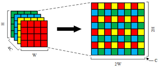
Figure 2.
Schematic diagram of the pixel shuffle.
2.3. Superpixel Segmentation
Superpixel segmentation divides the pixels in the image into clusters according to the similarity, which is a method of over-segmentation. However, this segmentation method lacks semantic information and cannot automatically merge the clusters of the same categories. The same target objects may be divided into multiple clusters. But it can accurately segment the boundaries of different target objects. The most classic superpixel segmentation method is the simple linear iterative clustering (SLIC) [55] proposed by Achanta et al. SLIC converts the RGB image to the CIELab color space and adds the initial XY coordinates of each superpixel cluster to form 5-dimensional features (XYLab). Then, SLIC uses the k-means clustering method to update the XY coordinates through multiple iterations to obtain the superpixel segmentation results.
Based on the SLIC, some improved versions, including the LSC [56] and Manifold-SLIC [57] algorithms, mainly improve the initial features. Achanta et al. [58] propose the simple non-iterative clustering SNIC based on the SLIC, which can run superpixel segmentation without iteration. Liu et al. [59] proposed the ERS method to extract superpixels by maximizing the entropy rate of pixels. Bergh et al. [60] proposed the SEEDS method, which is faster than SLIC. However, the parameter settings have a significant impact on the results. All of the above methods are based on artificially designed features for superpixel segmentation. Tu et al. [61] proposed the SEAL method, which can learn the deep features. But this method is non-differentiable. Based on the SLIC, Jampani et al. [62] proposes superpixel sampling networks (SSN). SSN is a differentiable superpixel segmentation network, which solves the problem of differentiable end-to-end learning. SSN introduces the idea of supervised learning and uses semantic segmentation labels to train SSN. The superpixel segmentation results of SSN are closer to the semantic segmentation results. However, SSN is only for superpixel segmentation tasks. For complex semantic segmentation tasks, the feature extraction network of SSN is too simple to obtain enough semantic features.
Yang et al. [63] proposed the Spixel FCN, which does not need to iterate through k-means clustering and learns superpixel segmentation entirely through DCNN. However, it cannot run the task of semantic segmentation. Lv et al. [64] concatenated the SLIC results into the features of the semantic segmentation network, but the superpixel feature branch is not learnable. Yuan et al. [65] proposed a method that combines DCNN and superpixel segmentation to classify high-resolution images for land cover classification. This method learned semantic segmentation and superpixel segmentation features through two branches of DCNN and superpixel FCN, respectively. It fused the features of the two branches to obtain semantic segmentation results. Mi et al. [66] proposed a deep neural forest method based on superpixel optimization, which performs semantic segmentation on very-high-resolution images. On mid-resolution images, due to the insufficient feature extraction capability of DCNN, the latter two methods do not perform as well as the results on high-resolution images.
3. Methodology
In order to solve the problem of insufficient feature extraction capability and inaccurate boundary details of DCNN on mid-resolution remote sensing images, we propose a novel DCNN architecture called block shuffle network (BSNet) and introduce superpixel segmentation to optimize the fine-grained boundary of target objects. The details of BSNet architecture are shown in Figure 3. We use UNet as the baseline network. In order to improve the feature extraction ability of the network for small target objects, we design the block shuffle structure as a parallel branch to upsample and reorganize the input data. In order to refine the boundaries fine-grained of target objects, we design the deep superpixel subnetwork to perform superpixel segmentation on the features extracted by the encoder and use the gradient of the superpixel branch to assist in optimizing the features of semantic segmentation. In order to optimize the semantic segmentation results with superpixel segmentation results at the end of the network, we design a self-boosting method to improve the fine-grainedness of semantic segmentation boundaries further.
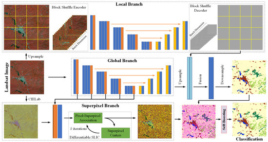
Figure 3.
Overview of the block shuffle network (BSNet) architecture.
3.1. Block Shuffle Structure
Since UNet belongs to the encoder-decoder style network, it has low memory overhead, fast running speed, and robust scalability. Therefore, we choose UNet as the baseline network. We choose ResNet-50 as the encoder of UNet for feature extraction. ResNet-50 will downsample the feature five times, the output feature map size is 1/32 of the input image, and the position and boundary details of the small target objects will become inaccurate. As shown in Figure 4, there are many small targets at mid-resolution images, such as Landsat images. We could reduce the number of downsampling. However, the features cannot be further aggregated and abstracted, the receptive field of the network cannot be effectively increased. The network cannot learn the necessary global information. We could maintain the ResNet-50 network structure as the original. That means the input data is directly upsampled, turning the small target objects into large target objects for training. It can improve the feature extraction ability of the network for small targets to a certain extent. We assume that our input data size is pixels, the encoder outputs a feature map of pixels after extracting features. At this time, the network has a strong ability to express global information. After upsampling the input data four times, we obtained new data with pixels. The encoder extracts the features and outputs a pixels feature map. At this time, the receptive field of the network is reduced by four times compared with the previous solution, and the global information aggregation degree is not enough. The global information is necessary for some large-range distributed target objects, such as woodland and cultivated land.

Figure 4.
Small target objects in Landsat images. (a) The pseudocolor Landsat image. (b) The semantic segmentation label.
Based on the UNet architecture, we introduce a new parallel branch and obtain a two-branch network. One of the branches still passes the data through the encoder to extract features and the decoder to fuse the low-level spatial position features and the high-level abstract features in a common way. This branch is called the global branch. The other branch is used for upsampling and pre-encoding the input data to improve the feature representation ability of the network from the data level. Inspired by the idea of pixel shuffle, we slice the upsampled input data, and each slice has the same size as the original data. Unlike the regular operation of concatenating tensors in the channel dimension, we concatenated sliced tensors in the batch dimension. Keeping the slice size consistent with the original input data size enables the encoder to maintain the aggregate abstraction capability of global features. We call this slicing and concatenating operation block shuffle encoder. After the feature map passes through the UNet decoder, the tensor is disassembled from the batch dimension, re-expanded and stitched into a large tensor of the same size as before block shuffle encoding. We call this disassembling and stitching operation block shuffle decoder. This branch is called the local branch. The global branch maintains the network’s original global receptive field size, which makes the network have a better feature extraction effect for large-scale objects. The local branch maintains the features of small targets, while avoiding the problem of insufficient feature aggregation caused by training an overly large image. Although both branches use the same UNet architecture for feature learning, the weights are independent of each other. Because the feature scales of the two branches are different, not sharing weights can avoid feature learning confusion. The feature map output by the global branch decoder is upsampled to the same size as the local branch. Then, we fused the two branch features. The network can express large-scale target objects and small target objects simultaneously. The details of the block shuffle encoder and block shuffle decoder are shown in Figure 5. The feature tensor size in block shuffle encoder and block shuffle decoder are shown in Table 1.
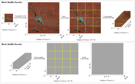
Figure 5.
Details of the block shuffle encoder and decoder. Since the input data of the decoder consitute the high-level feature map, we use gray blocks to represent the feature map.

Table 1.
Feature tensor shape in block shuffle encoder and block shuffle decoder.
3.2. Superpixel Branch
Since superpixel segmentation can cluster the input data, the boundaries of different target objects can be segmented very finely. The traditional SLIC method only performs clustering iterations from the CIELab color space of the original image, which is an unsupervised learning method. However, semantic segmentation labels can be used as supervised learning samples for superpixel segmentation. The semantic information cannot be obtained by superpixel segmentation. However, most superpixel segmentation boundaries should be completely coincident with the semantic segmentation boundaries. Inspired by the SSN, we add a differentiable SLIC branch in BSNet. We fuse the features extracted by the global branch encoder, the initial superpixel coordinates XY, and the CIELab color space of the input data. The fused feature is used for the input of the differentiable SLIC module. Then, the differentiable SLIC module outputs the superpixel features. We use semantic segmentation labels to calculate the superpixel gradients. Finally, we use the gradients to update the weights of the entire differentiable SLIC module. This branch is called the superpixel branch.
However, there is a contradiction between superpixel high-level features and semantic segmentation high-level features. In the superpixel feature, the pixels in each superpixel cluster have the same value, and the values of different clusters are different. In the semantic segmentation feature, the pixels of each category of target objects have the same value, and the pixel values of different categories are different. At the same time, the superpixel value does not have semantic information. It is only numbered from 1 and the upper left corner. Therefore, the corresponding relationship between the semantic segmentation category value and the superpixel value is not fixed on different images. There may be cases where the same category of target objects corresponds to multiple unfixed superpixel values, which will cause confusion in the semantic segmentation features. In order to avoid the mutual interference between the semantic segmentation task head and superpixel segmentation task head, we pull low-level features from the encoder of the global branch to the superpixel branch, not pulling the high-level features from the decoder. The gradient of the superpixel branch is backpropagated into the encoder to assist in optimizing the features and results of semantic segmentation.
As shown in Figure 6, we pull out the features of each stage in the encoder of the global branch. Assuming the encoder uses ResNet-50, the feature channels output by each stage are 64, 256, 512, 1024, 2048. We use a convolution to unify the number of channels to 64. Then we upsample the feature maps to the same size as the original input and concatenate them in the channel dimension to obtain a 320-dimension fused feature. We concatenate the initial superpixel coordinates XY with the CIELab color space of the input data to obtain a 5-dimensional feature. Then we concatenate the 320-dimension and 5-dimensional features to obtain a 325-dimensional feature. Finally, we use convolution to exchange feature information internally. We feed the fused features into the differentiable SLIC module. After k iterations, The differentiable SLIC module outputs the superpixel segmentation result.

Figure 6.
Details of the superpixel branch.
According to the differentiable SLIC in SSN, a soft association can be established between pixel and superpixel. The soft association can be expressed as follows:
where t represents the number of iterations, represents the 325-dimensional fused feature, and represents the center of superpixel cluster after iterations. can be updated by the weighted sum of pixel features, which can be expressed as follows:
where represents the number of pixels in the superpixel cluster, which is a normalization constant.
We use R to represent the semantic segmentation labels. Then, we use the column-normalized association matrix to map the pixel features to the superpixel features, . After iterations, we use the row-normalized association matrix to map the superpixel features back to the pixel features, . represents the superpixel reconstruction result. The entire reconstruction process can be expressed as follows:
In the differentiable SLIC module, three hyperparameters need to be set before training. represents the max number of iterations. represents the number of superpixel clusters. represents whether to merge small superpixel clusters into adjacent large ones. We will discuss the impact of these three hyperparameters in Section 5.2.
3.3. Self-Boosting Method
Since semantic segmentation and superpixel segmentation only share the encoder features of the global branch, the task heads are entirely different. Although the two tasks can assist each other in feature extraction, some information that the network considers useless may still be dropped in the task decoding stage. Each pixel inside the superpixel cluster has very similar characteristics, so we can regard the whole cluster as the same type of target object. As shown in Figure 7, the result of semantic segmentation is relatively smooth, and fits poorly with the natural boundary. There is also wrong noise inside the red region. The edge of the result of superpixel segmentation is relatively fine, which is consistent with the real natural scene, but the whole target object is divided into five clusters. The contour of the superpixel cluster is close to the real contour of the ground object, so we can assign semantic information with categories to the superpixel clusters. Since the red object is the dominant class, we assign each pixel of the superpixel cluster to the red class. It effectively eliminates the noise of internal errors and makes the edge contour more precise. Therefore, we can use superpixel segmentation results to optimize semantic segmentation results further.
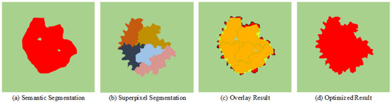
Figure 7.
Schematic diagram of optimizing semantic segmentation results by superpixel segmentation result. (a) The result of the semantic segmentation. (b) The result of the superpixel segmentation. (c) The overlay result (yellow represents the esult of the semantic segmentation, red represents the result of the superpixel segmentation). (d) The optimized result of semantic segmentation.
First, we obtain the region of each superpixel cluster. We construct a region matrix to represent the ith cluster. The position of the cluster is set to 1, and the rest are set to 0.
where represents the result of superpixel segmentation, ← represents the assignment operation, and .
Then, the same region in the semantic segmentation result is taken out using the region matrix .
where represents the result of semantic segmentation, · represents the dot multiply operator, and .
Then, we count the number of each class in the matrix and compute the highest number of class index .
where n represents the number of classes in the semantic segmentation labels, function can compute the index of maximum of , , , and .
Finally, we use to update the elements of the corresponding cluster in semantic segmentation result.
where .
We call this algorithm self-boosting. The algorithm essentially adds semantic information to the superpixel segmentation results. Therefore adjacent superpixel clusters of the same category are automatically merged. The algorithm also retains the fine boundaries in the superpixel segmentation results.
3.4. Loss Function
For the semantic segmentation task, the size of the feature map after fusion of the global branch and local branch is the same as the size of the upsampled input data. We also upsample the semantic segmentation labels to the same size to calculate the loss for supervised learning with more detailed information. We use cross-entropy and Lovász-softmax [67] loss as the loss function of BSNet.
The cross-entropy loss is calculated by
where N represents the total number of samples, represents the probability that the ground truth is true, represents the probability that the ground truth is false, represents the probability that the forward propagation result is true, and represents the probability that the forward propagation result is false.
The region-level loss can optimize the features as whole target objects in the semantic segmentation task. However, the cross-entropy loss is the pixel-level loss. Therefore, we also use the Lovász-softmax loss to train the network. Lovász-softmax loss is a smoothed Jaccard loss. The Jaccard index is the Intersection over Union (IoU). The Jaccard index of class c can be expressed as follows:
where y represents the ground truth labels, and represents the predicted labels.
Then, the Jaccard index is performed with smooth extensions. The mispredicted pixels for class c can be expressed as follows:
where y represents the ground truth labels, and represents the predicted labels.
At this time, Jaccard loss is smoothed as follows:
where y represents the ground truth labels, and p represents the forward probability.
Then, the smoothed Jaccard index can be expressed via error vector as follows:
where represents the probability of class c, and .
In order to ensure the class-averaged mean IoU (mIoU) metric, Lovász-softmax loss is finally defined as follows:
Combined with the cross-entropy loss, the semantic segmentation task loss is expressed as follows:
We adopt the reconstruction loss and compactness loss in SSN for the superpixel segmentation task. The reconstruction loss is to calculate the cross-entropy loss between the semantic segmentation label R and the superpixel reconstruction result , which can be expressed as follows:
where R represents the semantic segmentation labels, represents the superpixel reconstruction result, represents the column-normalized association matrix, and represents the row-normalized association matrix.
Compactness loss is used to make superpixel clusters to be spatially compact. We use to represent the positional pixel features. First, we use the column-normalized association matrix to map the positional features to superpixel features, . Then, we use hard association H instead of soft association Q, map the superpixel features back to pixel features, . Finally, the compactness loss is expressed as follows:
Combined with reconstruction loss, the superpixel segmentation loss is expressed as follows:
where represents the regularity of superpixel clusters, which is a hyperparameter for adjusting the degree of compactness.
Finally, the loss function for BSNet can be expressed as follows:
where represents the weight of superpixel loss, which is a hyperparameter for adjusting the order of magnitude balance of the two losses, which is more conducive to the learning and convergence of the network.
3.5. Evaluation Metrics
The overall accuracy (OA) is the ratio of the number of correctly classified pixels to the total number of pixels. The OA can be expressed as follows:
where y represents the ground truth labels, and represents the predicted labels.
The accuracy of each category is evaluated using the score. In the confusion matrix [68], true positives (TPs) are the elements on the main diagonal, false positives (FPs) are the sum of the elements in each column except the elements on the main diagonal, and false negatives (FNs) are the sum of the elements in each row except the elements on the main diagonal. The and are calculated by the confusion matrix and can be defined as follows:
Therefore, the score is defined as follows:
Since the OA is not adequately sensitive to the small categories [69], the mean F1 score (mF1) is also used for an overall evaluation. The mF1 is the average F1 score of each category.
4. Experimental Results
4.1. Datasets
Since there is currently no publicly available large-scale Landsat semantic segmentation dataset, in order to test the performance and generalization ability of our proposed BSNet on large-scale Landsat images, we made two sets of Landsat datasets to test our proposed method. Our research area is located in parts of North China and parts of Southwest China. We downloaded 102 scenes of the 2010 Landsat-5 images and mosaiced the images of the study area, removing the redundant images outside the study area. We finally get 20 tiles of images, each with a size of 10,240 × 10,240 pixels. It covers two study areas. One is an area of approximately 1,440,000 and is between and between . We name it Region N. The other is an area of approximately 360,000 and is between and between . We name it Region SW. We labeled all the images at the pixel level, including seven categories: woodland (WO), grassland (GL), wetland (WE), waterbody (WB), cultivated land (CL), artificial surface (AS), and bare land (BL).
All labels were manually visually interpreted by a team of more than a dozen people and generated from ArcGIS polygons, which took about six months in total. Since many of the small features in Landsat cannot be identified by the naked eye, the work team also resorted to high-resolution satellite images of multiple time series for reference. To ensure that the labels are of high quality, the whole work team has basic knowledge of landcover, and some disputed label points have been confirmed through on-the-spot inspections.
The more difficult to label category is wetland, which looks between grassland and water body. We label those three categories according to the following criteria: (1) areas that are chronically water throughout the year are labeled as waterbody; (2) if there is water for more than two months of the year and there is also vegetation, it is labeled as wetland; (3) those with no water present, or with both water and vegetation appearing in less than two months, are labeled as grassland. According to this rule, we used multi-temporal high-resolution satellite images to help judgment and field investigations in some disputed areas. The textures of other categories are quite different and can be easily interpreted visually.
Because the distribution of target objects has a certain geographical correlation, that is to say, the distribution of target objects in adjacent geographical areas is similar. Therefore, if the training set and the test set are randomly divided based on all image slicing, the two datasets will have a strong geographical correlation, which will affect the evaluation of the generalization ability of the model. Therefore, the training dataset and the test dataset are completely independent of each other in terms of geographical distribution. As shown in Figure 8, we use the inner 4 tiles (IDs 2-2, 2-3, 3-2, 3-3) as the training and validation dataset, named Landsat core dataset (LSC dataset), and the outer 12 tiles (IDs 1-1, 1-2, 1-3, 1-4, 2-1, 2-4, 3-1, 3-4, 4-1, 4-2, 4-3, 4-4) as the test dataset to evaluate the generalization ability, named Landsat extend dataset (LSE dataset). To further evaluate the generalization ability of our proposed method, we choose the images in Region SW for prediction, which is farther from Region N. As shown in Figure 9, we use all 4 tiles (IDs 5-1, 5-2, 5-3, 5-4) as the test dataset to evaluate the generalization ability, named Landsat supplement dataset (LSS dataset).
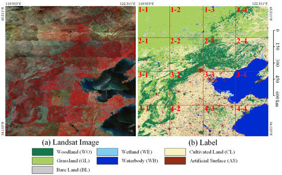
Figure 8.
Geographical distribution of Landsat core dataset and Landsat extend dataset in Region N. LSC dataset IDs: 2-2, 2-3, 3-2, 3-3. LSE dataset IDs: 1-1, 1-2, 1-3, 1-4, 2-1, 2-4, 3-1, 3-4, 4-1, 4-2, 4-3, 4-4. (a) Landsat images. (b) Labels.
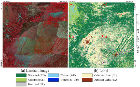
Figure 9.
Geographical distribution of Landsat supplement dataset in Region SW. LSS dataset IDs: 5-1, 5-2, 5-3, 5-4. (a) Landsat images. (b) Labels.
4.2. Implement Details
4.2.1. Data Preprocessing
To train the LSC dataset, we perform sliding window cropping on the big tiles to obtain 25,600 small tiles with pixels. We randomly divided the cropped LSC dataset into the training set and validation set with the ratio of 8:2. Since the input data size correlates with the hyperparameter in the superpixel branch of our proposed BSNet. In order to ensure that the superpixel branch is consistent in the inference phase and the training phase, we also perform the same sliding window cropping on the LSE dataset to obtain 76,800 small tiles with pixels. All bands of data are used for training and prediction.
According to Equation (25), we normalize the multi-spectral Landsat input data to speed up the model convergence.
where represents the normalized data, D represents the input data, represents the mean value of the corresponding channel in the input data, and represents the standard deviation of the corresponding channel in the input data.
4.2.2. Training Settings
We use the PyTorch deep learning framework [70] to implement many published mainstream models and the BSNet proposed in this paper. We use four NVIDIA RTX 3090 GPUs for training, and the memory of the GPU is 24 GB. We use random horizontal flip, random vertical flip, and random rotation as the data augmentation methods. The batch size is set to 16. We choose Adam as the optimizer with betas set to default values of 0.9 and 0.999, eps set to a default value , and weight decay set to . The learning rate uses the warm-up strategy and reduce-LR-on-plateau strategy. The initial learning rate is set to . According to the warm-up strategy (see Equation (26)), the learning rate rises to at the 10th epoch. Then, according to the reduce-LR-on-plateau strategy (see Equation (28)), when the validation accuracy is no longer improved in every 20 epochs, the learning rate is multiplied by 0.3. The training is stopped when the learning rate is lower than .
where presents the current learning rate, represents the initial learning rate, represents the learning rate at the end of the warm-up strategy, t represents the current number of iterations, and n represents the total number of iterations in the warm-up strategy. n is calculated as follows:
where e represents the total number of epochs in the warm-up strategy, and k represents the number of iterations per epoch.
where represents the current learning rate, represents the last old learning rate, and represents the factor in the reduce-LR-on-plateau strategy.
For the hyperparameters in BSNet, the upsample scale in block shuffle structure is set to 4. In superpixel branch, is set to 1024, is set to 10, and is set to false. In loss function, is set to 0.01, and is set to 1. To avoid random errors in the training stage, we trained all models 10 times to calculate the average accuracy of each model.
4.3. Experiments on the Landsat Core Dataset
4.3.1. Ablation Study
We gradually integrate the modules and structures proposed in this paper on the baseline UNet to show the effects of each module and structure. Table 2 shows the quantitative accuracy evaluation of our method on the validation set of the LSC dataset. The baseline is UNet using ResNet-50 as encoder, and the OA is 81.3%. Based on UNet, we added a block shuffle structure as the local branch to build a basic BSNet. The upsample scale is set to 4. The block shuffle structure can improve the feature extraction ability of the network for small target objects and keep more feature details. Therefore, the accuracy of each category has been significantly improved, and the OA has increased to 83.7%. In order to test the performance of the superpixel branch, we added this branch to UNet and BSNet, respectively. We build UNet-SP and BSNet-SP networks, with the of 1024, of 10, and is false. Helped by the superpixel segmentation branch based on supervised learning of semantic segmentation labels, the encoder pays more attention to small target objects and more fragmented object features. The OA of UNet-SP reaches 83.9%, and the OA of BSNet-SP reaches 85.6%. In order to use the superpixel segmentation results to optimize the semantic segmentation results, we finally apply the self-boosting method to the UNet-SP and BSNet-SP networks and name them UNet-SP-SB and BSNet-SP-SB, respectively. As some small details of object boundaries are optimized, the OA reaches 84.8% and 86.3%, respectively. Compared with baseline UNet, our proposed best network architecture, BSNet-SP-SB, achieves 5.0% accuracy improvement.
Table 2.
The effect of the block shuffle structure, superpixel branch and self-boosting on Landsat core dataset.
The visualized comparison of our proposed block shuffle structure and superpixel branch on the LSC dataset is shown in Figure 10. In order to show more overall ground object distribution and effects, we stitched together four adjacent tiles of pixels to obtain one big tile of pixels. We used the stitched big tiles for visual analysis of the results. In the first row, when extracting the fragmented artificial surface by the UNet, there will be a lot of missed detections. Most of the grassland is classified as woodland. The small grass clusters in the upper left area cannot be extracted. The BSNet extracts more fragmented artificial surfaces and has a stronger ability to extract small target features than the UNet. However, the confusion between grassland and woodland is still a trouble. With the help of superpixel branch, the UNet-SP and the BSNet-SP can keep more details of small target objects in hidden layers of the network. So the ability to distinguish between grassland and woodland is improved. Thanks to the feature extraction ability of the block shuffle structure for small target objects, the BSNet-SP has more details than the UNet-SP. The fragmented grass in the upper left area has been extracted correctly.
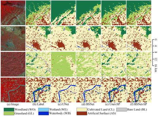
Figure 10.
Ablation study with the block shuffle structure and superpixel branch on Landsat core dataset. (a) Landsat image. (b) Ground truth. Inference result of (c) the UNet, (d) the UNet with the block shuffle structure (BSNet), (e) the UNet with the superpixel branch (UNet-SP), and (f) the BSNet with the superpixel branch (BSNet-SP).
In the second row, the UNet can only extract rough outlines for medium-sized towns, while the BSNet can extract richer outline details and interior texture structures. After adding the superpixel branch, the UNet-SP can extract more accurate contour details. The the BSNet-SP adds a more detailed optimization for the inner details of the town. For small villages, the UNet will have a large number of missed detections due to insufficient feature extraction capabilities for small target objects. The BSNet can extract most small villages, but the contours are relatively smooth. The UNet-SP and the BSNet-SP can optimize the outline details of small villages, making the classification results more in line with the natural geographical morphology.
In the third row, for the fragmented and staggered distribution of woodland, grassland, and cultivated land, the UNet cannot extract enough classification information since the features are very complex. Therefore, most of the areas are misclassified as grassland. The BSNet relies on strong feature extraction ability to distinguish most cultivated land from grassland, but there are still many missed detections for small villages. The UNet-SP and the BSNet-SP effectively distinguish woodland and grassland. The BSNet-SP has a higher extraction ability for small villages than the UNet-SP. The narrow river is successfully extracted by none of the four networks. So more research on slender targets is needed in the future.
In the fourth row, the UNet fails to extract slender roads. Many small villages are missed, and the boundaries of small and medium-sized contiguous townships are very rough. The BSNet successfully extracts slender roads and optimizes the edge contour details of villages and towns. However, some village features are still ignored. The UNet-SP and the BSNet-SP strengthen the attention to detail on small objects. Most of the villages and towns are extracted successfully, and the woodland next to the river is also correctly extracted. Without the help of the block shuffle structure, the UNet-SP has a poor road extraction effect and many disconnections in the road result. The BSNet-SP can extract the slender features of the road. It can be seen that our proposed block shuffle structure and superpixel branch are very effective for small and fragmented target objects on Landsat images.
The visualized comparison of our proposed self-boosting method on the LSC dataset is shown in Figure 11. Since this method mainly optimizes the classification results at the fine-grained edge, in order to show clearer details, we use small tiles of pixels for visual analysis of the results. In the first row, the edge contours of the UNet-SP and the BSNet-SP are relatively smooth because the semantic segmentation decoder cannot preserve the comparatively detailed edge position features. After using the superpixel segmentation results to refine the edge of the semantic segmentation results, the edges of the woodland and grassland extracted by the UNet-SP-SB and the BSNet-SP-SB are more refined and more in line with the natural geographic scene.
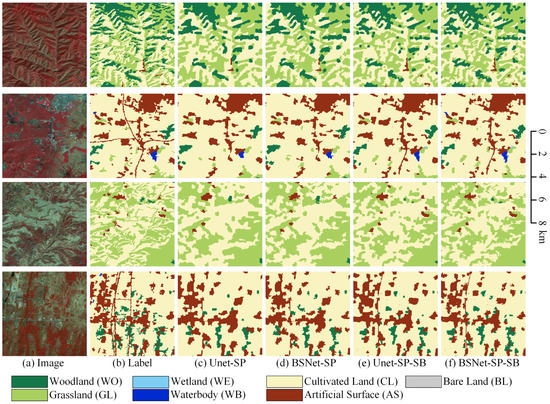
Figure 11.
Ablation study with the self-boosting method on Landsat core dataset. (a) Landsat image. (b) Ground truth. Inference result of (c) the UNet with the superpixel branch (UNet-SP), (d) the UNet-SP with the self-boosting method (UNet-SP-SB), (e) the BSNet with the superpixel branch (BSNet-SP), and (f) the BSNet-SP with the self-boosting method (BSNet-SP-SB).
In the second row, the outline should be rough for natural small villages and medium-sized towns. Although the UNet-SP and the BSNet-SP have retained more edge contour details, they are still smooth in the outlines. After optimized by superpixel segmentation results, the semantic information is re-adjusted at the edges, and the details are more realistic.
In the third row, grassland is a fragmented target object type, and villages are small target objects with complex edge contours. The UNet-SP and the BSNet-SP can only extract ground objects and relatively fine contours. The result of superpixel segmentation can finely fit the edges to the target object boundary. Therefore, the smooth semantic segmentation results can be optimized into high fine-grained classification results.
In the fourth row, the edges of small contiguous villages and inter-fragmented woodlands are more complex. Combining the semantic information with the refined edge contour information in superpixel segmentation can significantly optimize the results of complex edges. It can be seen that our proposed self-boosting method is very effective for fine-grained optimization of edge contours of classification results on Landsat images.
4.3.2. Comparing Methods
To compare with the mainstream semantic segmentation models, we trained many mainstream models on the LSC dataset and compared the results with our best BSNet-SP-SB model. Table 3 shows that 81.3% OA is the bottleneck of mainstream models, but the BSNet-SP-SB model can reach 86.3%. The accuracy of most categories is much higher than that of mainstream models, and the improvement is about 2.6–7.2% compared to the UNet.
Table 3.
Accuracy comparison between our BSNet and other methods on the Landsat core dataset.
The semantic segmentation models we compared are listed as follows:
- (1)
- UNet++: This method is proposed by Zhou et al. [71] The UNet++ adds more nodes to the UNet decoder and fuses features from different stages in a very dense form.
- (2)
- LinkNet: This method is proposed by Chaurasia et al. [72] The LinkNet achieves real-time semantic segmentation by reducing the complexity of the network and ensuring high accuracy.
- (3)
- PSPNet: This method is proposed by Zhao et al. [48] The PSPNet uses dilated convolutions to keep the resolution of feature maps, and uses the SPP module to extract features at different scales.
- (4)
- DeepLabV3+: This method is proposed by Chen et al. [73] The DeepLabV3+ is a hybrid architecture based on backbone-style and encoder-decoder-style networks. It uses atrous convolutions to keep the resolution of feature maps, and uses the ASPP module to extract features at different scales.
- (5)
- PAN: This method is proposed by Li et al. [74] The PAN uses the feature pyramid attention (FPA) module to extract features at different scales, and uses the global attention upsample (GAU) module to fuse features at different stages.
- (6)
- UNet: This method is proposed by Ronneberger et al. [51] The UNet keeps the features of each stage in the encoder, gradually upsample and restore the pooled features in the decoder, and fuse them with the low-level features of the corresponding stage in the encoder.
- (7)
- BSNet: Our BSNet is the UNet with the block shuffle structure, the superpixel branch, and the self-boosting method. For convenience, we note the BSNet-SP-SB in Section 4.3.1 as BSNet here.
The visualized comparison of the mainstream models and our proposed BSNet model on the LSC dataset is shown in Figure 12. In order to show more overall ground object distribution and effects, we stitched together four adjacent tiles of pixels to obtain one big tile of pixels. We used the stitched big tiles for visual analysis of the results. In the first row, the distribution of woodland, grassland, cultivated land, and small villages is complex. The mainstream models cannot effectively extract and maintain small target features and fine-grained features, so the grassland classification results are erroneously combined together, and the cultivated land reversely occupies the grassland. Some smaller villages are missed. With the help of the block shuffle structure and the superpixel branch, our proposed BSNet optimizes extracting and keeping detailed features. It can effectively distinguish grassland and cultivated land and extract smaller villages.
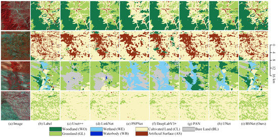
Figure 12.
Some examples of the results on the Landsat core dataset. Comparison between our BSNet and other methods. (a) Landsat image. (b) Ground truth. Inference result of (c) the UNet++, (d) the LinkNet, (e) the PSPNet, (f) the DeepLabV3+, (g) the PAN, (h) the UNet, and (i) our proposed BSNet.
In the second row, medium-sized towns and small villages are distributed in flecks and fragments, which requires the network to extract small objects and keep features. The results of the mainstream models will link the artificial surface areas together and ignore most of the cultivated land between the artificial surfaces. Also, some very small villages have been missed. Our proposed BSNet effectively extracts these fragmented cultivated land features, solves the problem of missed detection of cultivated land, and greatly optimizes the results of small villages.
In the third row, grassland, woodland, bare land, cultivated land, and wetlands are very complex and intertwined. There are also several small villages in this complex scene. When the mainstream models face such a complex scene, the features of small targets are easily occupied by the features of large targets. Therefore, in the classification results of the mainstream models, some particular ground objects will dominate in the whole scene, and many small target objects will be misclassified and ignored. For example, it is wrongly classified as the wrong combination of bare land/grassland, wetland/bare land, and wetland/woodland. Our proposed BSNet effectively distinguishes complex objects, correctly classifies complex scenes, and keeps the features of small targets simultaneously.
In the fourth row, grassland and cultivated land are fragmented together, with grassland more dispersed and cultivated land more aggregated. Therefore, the cultivated land encroaches on the grassland in the result of the mainstream models. That is, many grasslands are wrongly classified into cultivated land. Our proposed BSNet has a stronger ability for small target feature extraction and fine-grained retention. Therefore, the fragmented grassland is extracted as much as possible, and the edge details are closer to the natural scene. Although there are still a small number of missed detections, a significant improvement has been achieved compared to the mainstream models.
4.4. Experiments on the Landsat Extend Dataset
4.4.1. Ablation Study
To test the generalization ability of the modules and structures proposed in this paper on Landsat images, we performed prediction and accuracy evaluation on the LSE dataset, which was not involved in the training stage. As shown in Table 4, the accuracy of all models is slightly lower than that of the LSC dataset. The reason is that the LSC dataset participated in the accuracy validation during the training phase. We selected the optimal model based on the accuracy of the validation set of the LSC dataset, and this model performed the best in the LSC dataset. However, if the LSE dataset does not participate in the training stage, it is normal that the accuracy will be relatively lower than that of the LSC dataset. Because the geographic distributions of the two datasets are relatively independent, a slight drop in accuracy indicates that the model has good generalization ability, otherwise the accuracy on the LSE dataset will drop significantly. Our proposed BSNet-SP-SB can still achieve 83.2% OA on the LSE dataset.
Table 4.
The effect of the block shuffle structure, superpixel branch and self-boosting on Landsat extend dataset.
The visualized comparison of our proposed block shuffle structure and superpixel branch on the LSE dataset is shown in Figure 13. In order to show more overall ground object distribution and effects, we stitched together four adjacent tiles of pixels to obtain one big tile of pixels. We used the stitched big tiles for visual analysis of the results. In the first row, the UNet misses many small fragmented woodland targets, and the artificial surface has rough outlines. The BSNet extracts a small part of finely fragmented woodland, and obtains more abundant artificial surface contour details. The UNet-SP and the BSNet-SP extracted most of the finely fragmented woodland, and greatly optimized the outlines of small villages and medium-sized towns.
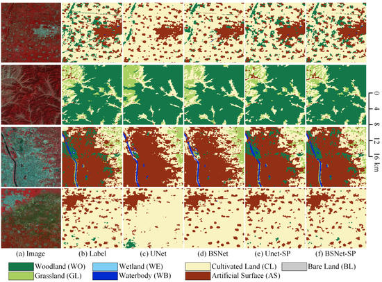
Figure 13.
Ablation study with the block shuffle structure and superpixel branch on Landsat extend dataset. (a) Landsat image. (b) Ground truth. Inference result of (c) the UNet, (d) the UNet with the block shuffle structure (BSNet), (e) the UNet with the superpixel branch (UNet-SP), and (f) the BSNet with the superpixel branch (BSNet-SP).
In the second row, grassland, cultivated land, and small villages are staggered in the upper left area. The UNet cannot effectively distinguish fragmented distributed features, all of which are classified as grassland. The BSNet can extract the outline of the grassland, but ignore most villages. The UNet-SP and the BSNet-SP correctly distinguish villages, and optimize the details of interlaced outlines of woodland and grassland in other areas.
In the third row, in the large city scene, the UNet will ignore other small targets in the middle of the city, and the contours of most target objects are relatively smooth. The BSNet has improved some fine-grained features in the city area, such as smaller woodlands and urban-rural fringe where cultivated land and towns are staggered together. The UNet-SP and the BSNet-SP extract more small target objects in the city. The large woodland in the upper left area and the intertwined area of the woodland/city on the right are all correctly extracted. Compared with the UNet-SP, the BSNet-SP can keep more small target features.
In the fourth row, many small villages are ignored by the UNet. The BSNet extracts most villages, but their edge contours are relatively smooth and incorrect. The UNet-SP and the BSNet-SP significantly optimize the outlines of small villages and medium-sized towns, making the boundaries more in line with the natural shapes of objects. It can be seen that our proposed block shuffle structure and superpixel branch have good generalization ability on Landsat images.
The visualized comparison of our proposed self-boosting method on the LSE dataset is shown in Figure 14. Since this method mainly optimizes the classification results at the fine-grained edge, in order to show clearer details, we use small tiles of pixels for visual analysis of the results. In natural scenes, for cultivated forests, grasslands, small villages, and medium-sized towns with complex edge contours, the sawtooth shape at the edge is more in line with the natural geographical scene. Since the decoder for semantic segmentation loses jagged-shape details during upsampling, the semantic segmentation results are inevitably smooth. Using the results of superpixel segmentation to refine and correct the boundaries of semantic segmentation can greatly improve the fine-grainedness of segmentation results. It can be seen that our proposed self-boosting method has good generalization ability on Landsat images.
Figure 14.
Ablation study with the self-boosting method on Landsat extend dataset. (a) Landsat image. (b) Ground truth. Inference result of (c) the UNet with the superpixel branch (UNet-SP), (d) the UNet-SP with the self-boosting method (UNet-SP-SB), (e) the BSNet with the superpixel branch (BSNet-SP), and (f) the BSNet-SP with the self-boosting method (BSNet-SP-SB).
4.4.2. Comparing Methods
To test and compare the generalization ability of the mainstream model and the BSNet-SP-SB proposed in this paper, we performed predictions and accuracy evaluations on the LSE dataset, which did not participate in the training stage. As shown in Table 5, the accuracy of all models decreases slightly on the LSE dataset. Even so, our proposed BSNet-SP-SB still surpasses other mainstream models on the LSE dataset, with an accuracy of 83.2%. The mainstream semantic segmentation models are the same as Section 4.3.2. For convenience, our BSNet-SP-SB is still noted as BSNet here.
Table 5.
Accuracy comparison between our BSNet and other methods on the Landsat extend dataset.
The visualized comparison of the mainstream models and our proposed BSNet model on the LSE dataset is shown in Figure 15. In order to show more overall ground object distribution and effects, we stitched together four adjacent tiles of pixels to obtain one big tile of pixels. We used the stitched big tiles for visual analysis of the results. In the first row, the mainstream models lose the features of small villages and grassland in the network. Therefore, these two categories of target objects are ignored or occupied by cultivated land. Our proposed BSNet effectively extracts the features of these small objects. In mainstream models, many patchy cultivated land inside medium-sized towns will be occupied by artificial surfaces. In our method, most of them are correctly classified.
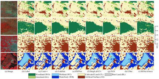
Figure 15.
Some examples of the results on the Landsat extend dataset. Comparison between our BSNet and other methods. (a) Landsat image. (b) Ground truth. Inference result of (c) the UNet++, (d) the LinkNet, (e) the PSPNet, (f) the DeepLabV3+, (g) the PAN, (h) the UNet, and (i) our proposed BSNet.
In the second row, there are many small grassland targets in the large woodland in the middle area, which is an absolute advantage over the grassland. The mainstream models wrongly classify them into the woodland. The cultivated land around the woodland is mixed with many small village targets. The mainstream models are also unable to extract all the villages effectively. Our proposed BSNet can effectively extract the small objects that are geographically disadvantaged to surrounding objects. It also shows that our method is very effective for small object extraction.
In the third row, some small grasslands, woodlands, and water bodies are mixed in large cities. The mainstream models cannot extract these small objects, and the cities occupy these small objects in the result. Our proposed BSNet can still separate these small objects from the dominant large ones. Besides, our edge details are also more accurate in the surrounding small villages.
In the fourth row, the wetland features are similar to other categories, but the mainstream models have limited feature extraction ability to distinguish similar features. Therefore, the wetlands are wrongly classified into other categories in the result. The UNet can extract wetlands correctly, but there are still misclassified water bodies inside the wetlands. Our proposed BSNet has the stronger feature extraction ability and can keep more details of features. So, the wetlands are successfully discriminated against from other classes in the result.
4.5. Experiments on the Landsat Supplement Dataset
To further test the generalization ability of the modules and structures proposed in this paper on Landsat images, we performed prediction and accuracy evaluation on the LSS dataset, which was further away from the training region. As shown in Table 6, the accuracy of all models is lower than that of the LSC dataset and LSE dataset. The reason is that Region SW is far away from Region N. There will be some scenes in the image that have not appeared in the training set. Since DCNN is a fully data-driven supervised learning method, there may be a reduction in accuracy in the face of unseen scenarios. However, the reduction in accuracy is relatively small. We believe that the model still has good generalization ability. Our method can still achieve 73.4% on the LSS dataset. The visualized comparison of the mainstream models and our proposed BSNet model on the LSS dataset is shown in Figure 16. Our proposed BSNet has better performance for small objects and feature boundaries.
Table 6.
Accuracy comparison between our BSNet and other methods on the Landsat supplement dataset.

Figure 16.
Some examples of the results on the Landsat supplement dataset. Comparison between our BSNet and other methods. (a) Landsat image. (b) Ground truth. Inference result of (c) the UNet++, (d) the LinkNet, (e) the PSPNet, (f) the DeepLabV3+, (g) the PAN, (h) the UNet, and (i) our proposed BSNet.
4.6. Large-Scale Landcover Mapping
We use the trained BSNet-SP-SB model with the highest accuracy to predict all the 16 tiles of Landsat images in the study area Region N. All prediction results are optimized with superpixel segmentation results through the self-boosting method. Finally, we stitch the classification results into a large map, as shown in Figure 17.
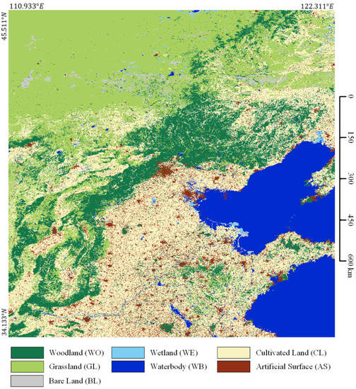
Figure 17.
Large-scale classification results in parts of North China.
We also use the trained BSNet-SP-SB model with the highest accuracy to predict all the 4 tiles of Landsat images in the study area Region SW, as shown in Figure 18. It shows that our proposed BSNet has a good generalization ability in Landsat images.
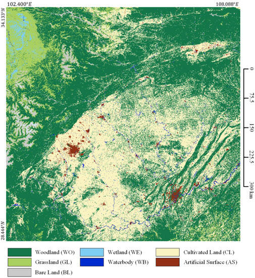
Figure 18.
Large-scale classification results in parts of Southwest China.
5. Discussion
5.1. Trade-Off in the Block Shuffle Structure
In the block shuffle structure, upsample scale significantly impacts model accuracy and running efficiency. When the upsample scale is two times the original, the computational overhead will reach four times. Although the model accuracy will increase with the upsample scale, choosing between the computational cost and the model accuracy is a trade-off problem.
We choose the upsample scale as 1, 2, 4, and 8 for comparative experiments. The correspondence between upsample scale, GPU memory overhead, training/prediction duration, and accuracy on the LSC dataset is shown in Table 7. The upsample scale equals 1 as the reference baseline.
Table 7.
The correspondence between upsample scale, GPU memory overhead, training/prediction duration, and accuracy on the LSC dataset.
We can find that with the increase of the upsample scale, the computation resources, and running time overhead increase exponentially, but the model accuracy is improved less and less. The visualized comparison of different upsample scale values is shown in Figure 19. When the upsample scale is set to 2, the small target features extracted by the network have improved, but some small objects are still missing. When the upsample scale is set to 4, the network can extract more small target features, such as very small villages or slender rivers and roads. When the upsample scale is set to 8, the improvement is very slight, and there is no noticeable improvement in the result. Combined with its computing overhead, the cost is too high to set a big upsample scale value.
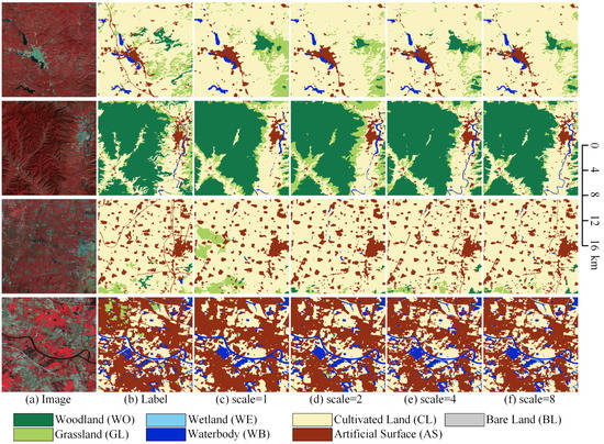
Figure 19.
The visualized comparison of different upsample scale values on the Landsat core dataset. (a) Landsat image. (b) Ground truth. Inference result of (c) the BSNet with the upsample scale is 1, (d) the BSNet with the upsample scale is 2, (e) the BSNet with the upsample scale is 4, and (f) the BSNet with the upsample scale is 8.
Therefore, we do not need to set the upsample scale too large in real projects. In this paper, we set the upsample scale to 4 to improve the network feature extraction capability while keeping the computational resources within an acceptable range.
5.2. Hyperparameters in Superpixel Branch
represents the number of superpixel clusters. If this parameter is set too small, different types of ground objects will be forced to be classified into the same superpixel clusters. It results in wrong merging when using superpixel segmentation results to optimize semantic segmentation results. Setting too large will cause the same category of target objects to be segmented into too many small blocks. And it will also consume too much GPU memory computing resources. We counted the semantic segmentation labels in all samples, and the distribution of the number of target objects in each tile is shown in Figure 20.
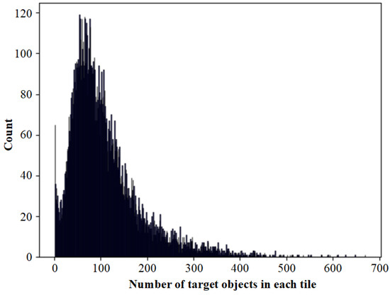
Figure 20.
The distribution of the number of target objects in each tile of the sample.
We can see that most samples contain pixels between 1 to 400. The peak is around 90, the maximum value is 670, and the case of more than 400 is rare. Since the initial positions of each superpixel cluster are regularly distributed in the image, there may be multiple superpixel clusters in the same target objects. Some smaller target objects may not match independent superpixel clusters without redundancy settings and are mistakenly merged into adjacent superpixel clusters. Therefore, we set to 1024, and there are 32 superpixel clusters in the height and width axis, which can solve the correspondence problem between most superpixel clusters and semantic target objects. The computational resource overhead caused by increasing the number of superpixel blocks to solve the remaining few clusters is not cost-effective.
represents the max number of iterations of the differentiable SLIC module. Since the position of superpixel clusters is iteratively updated through k-means clustering, the larger , the more accurate the superpixel segmentation results. When reaches a certain number, the segmentation results tend to be stable, and continuing iterations will not change the segmentation results. According to the SLIC and the SSN recommendations, generally, can be set to 10, and a larger value will only waste computing resources.
represents whether to merge small superpixel clusters into adjacent large ones during the inference stage. We counted the semantic segmentation labels in the samples, and the distribution of the pixel number by each target object is shown in Figure 21. In the small tiles sample of pixels, there may exist target objects with more than 60,000 pixels, such as large areas of woodland or waterbodies, but this situation is rare. Since superpixel segmentation is an over-segmentation method, it is inevitable that the same target objects will be divided into multiple clusters, so we do not need to consider the target objects with too many pixels. We take 500 pixels as the maximum value of the statistics, see the inner small histogram. However, the histogram is mainly distributed below 100, so we take 50 pixels as the maximum value of statistics, see the main histogram.
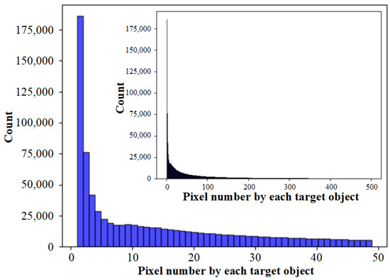
Figure 21.
The distribution of the pixel number by each target object.
We can find that there are many target objects with a pixel count of less than 10, and even more than 175,000 objects with only 1 pixel. There are also many small target objects between 10 and 50. If we forcibly merge the small superpixel clusters, small clusters may be merged into surrounding large clusters. If the two clusters themselves have different semantic information, the small target objects will be occupied by the large objects. Therefore, not merging small superpixel clusters is better for Landsat images. should be set to False. As shown in Figure 22, if is set to True, some small clusters are swallowed by the surrounding large clusters, resulting in more missed detections. Merging the small clusters is a negative optimization.
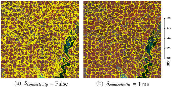
Figure 22.
The effect of on Landsat images. (a) is set to False. (b) is set to True.
5.3. Compactness Weight in Loss Function
represents the regularity of superpixel clusters. As shown in Figure 23, the larger is, the more regularity the superpixel cluster is, similar to the chessboard distribution. The smaller , the messier the superpixel cluster. The target objects in nature are not distributed in a regular checkerboard, and most of the target objects’ distribution is very messy, so should be set small. Superpixel segmentation will have an obvious checkerboard effect when is set too large, which is not suitable for the geographically natural scene with the fragmented distribution. In this paper, we set to 0.01, which has a good superpixel segmentation effect on Landsat images.
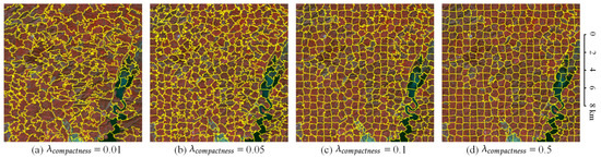
Figure 23.
The effect of on Landsat images. (a) is set to 0.01. (b) is set to 0.05. (c) is set to 0.1. (d) is set to 0.5.
5.4. Implications and Limitations
The BSNet proposed in this paper solves two problems encountered by DCNN in the semantic segmentation of mid-resolution remote sensing images. The first problem is that DCNN always ignores the small target objects. The second problem is that the edge contours of the target objects are smooth and not refined enough. The Block Shuffle structure enhances the Landsat image. It simulates the small target objects into larger target objects so that the network encoder can retain the features of the small target object without being lost. From the experimental results of this paper, the Block Shuffle structure can indeed effectively solve the problem of small target objects missing in Landsat images. This method is theoretically not limited to Landsat data, nor is it limited to mid-resolution images. It theoretically has enhanced effects on small targets on all types of remote sensing images. The Superpixel branch uses semantic segmentation labels to supervise the superpixel reconstruction, and the entire branch is learnable. The gradient of the superpixel branch can be passed to the semantic segmentation branch, and the two features are optimized and learned from each other. Therefore, it can also solve the missed detection of some small target objects and poor boundary details to a certain extent. Deep learning semantic segmentation is a purely data-driven method, while superpixel segmentation is a feature extraction guided by specific rules. Information that pure data-driven methods may lose can be extracted through guidance. Thus the two branches are complementary in methodology. The self-boosting algorithm optimizes the semantic segmentation results through the superpixel segmentation results. The results of semantic segmentation are smooth, and the results of superpixel segmentation are more accurate but have no semantic information. The two results just complement each other and optimize each other, which solves the problem that the edge contour of the target object is not fine enough. This method is also not limited to mid-resolution images and works in all pixel-level classification scenarios. The more complex the target contour, the better the effect. In addition to the above two problems that appear in mid-resolution images, there may be problems with small target objects and imprecise contours in the entire field of remote sensing deep learning. Therefore, the BSNet proposed in this paper can solve the general problems of remote sensing deep learning and improve the performance of deep learning methods.
However, BSNet also has some flaws. The GPU computing resource overhead of BSNet is too large, and the calculation speed is slow. Although the superpixel branch extracts features from the semantic segmentation encoder, the two branches remain independent of each other. The two branches are not completely unified at the level of loss function optimization to learn features together. Because of this defect, the final result needs to be optimized by the self-boosting method and cannot run BSNet training or inference by the complete end-to-end process.
In future research, we will focus on more important features in the block shuffle module, reduce feature redundancy, and try to optimize GPU computing resource overhead. We will try to design a new loss function that calculates both semantic segmentation loss and superpixel loss from the loss function level. So that semantic segmentation and superpixel segmentation can learn as a whole, fully share feature weights, optimize each other, and realize end-to-end training and inference. We will try to conduct experiments on different data sources to find general problems that BSNet can solve in remote sensing deep learning. We will not be limited to superpixels. We can try more feature extraction schemes with specific rules and combine them with deep learning methods to solve more problems.
6. Conclusions
In this paper, we proposed a novel semantic segmentation method for Landsat images. We designed a block shuffle structure to enhance the features of mid-resolution images and improve the feature extraction capability of DCNN. We designed a superpixel branch to supervise the superpixel segmentation with semantic segmentation labels, thereby assisting the optimization of the feature extraction and improving the accuracy of semantic segmentation. We designed a self-boosting method that integrates the semantic information of the semantic segmentation results and the precise boundary information of the superpixel segmentation results, which improves the fine-grainedness of the final segmentation results. Our experiments with our proposed BSNet on our self-made large-scale Landsat land cover dataset achieved state-of-the-art performance compared to other methods. In future research, we will promote our proposed BSNet to more datasets.
Author Contributions
X.Y. wrote the manuscript, designed the methodology, developed the codes, and conducted experiments; Z.C. and B.Z. supervised the study and reviewed the manuscript; B.L. preprocessed the data of the study area; Y.B. and P.C. made the datasets. All authors have read and agreed to the published version of the manuscript.
Funding
This research was supported by the Strategic Priority Research Program of the Chinese Academy of Sciences under Grant No. XDA19080302.
Institutional Review Board Statement
Not applicable.
Informed Consent Statement
Not applicable.
Data Availability Statement
Not applicable.
Acknowledgments
The authors thank the editors and anonymous reviewers for their valuable comments, which greatly improved the quality of the paper.
Conflicts of Interest
The authors declare no conflict of interest.
Abbreviations
The following abbreviations are used in this manuscript:
| DCNN | deep convolutional neural network |
| NDVI | normalized difference vegetation index |
| NDWI | normalized difference water index |
| NDBI | normalized difference built-up index |
| BSNet | block shuffle network |
| SSN | superpixel sampling network |
| SPP | spatial pooling pyramid |
| ASPP | atrous spatial pyramid pooling |
| SLIC | simple linear iterative clustering |
| IoU | Intersection over Union |
| mIoU | mean Intersection over Union |
| WO | woodland |
| GL | grassland |
| WE | wetland |
| WB | waterbody |
| CL | cultivated land |
| AS | artificial surface |
| BL | bare land |
| LSC dataset | Landsat core dataset |
| LSE dataset | Landsat extend dataset |
| LSS dataset | Landsat supplement dataset |
| OA | overall accuracy |
| TP | true positive |
| FP | false positive |
| FN | false negative |
| mF1 | mean F1 score |
References
- Ma, Y.; Wu, H.; Wang, L.; Huang, B.; Ranjan, R.; Zomaya, A.; Jie, W. Remote sensing big data computing: Challenges and opportunities. Future Gener. Comput. Syst. 2015, 51, 47–60. [Google Scholar] [CrossRef] [Green Version]
- Zhang, B. Remotely sensed big data era and intelligent information extraction. Geomat. Inf. Sci. Wuhan Univ. 2018, 43, 1861–1871. [Google Scholar]
- Zhang, B.; Chen, Z.; Peng, D.; Benediktsson, J.A.; Liu, B.; Zou, L.; Li, J.; Plaza, A. Remotely sensed big data: Evolution in model development for information extraction [point of view]. Proc. IEEE 2019, 107, 2294–2301. [Google Scholar] [CrossRef]
- Li, L. Deep residual autoencoder with multiscaling for semantic segmentation of land-use images. Remote Sens. 2019, 11, 2142. [Google Scholar] [CrossRef] [Green Version]
- Lv, N.; Zhang, Z.; Li, C.; Deng, J.; Su, T.; Chen, C.; Zhou, Y. A hybrid-attention semantic segmentation network for remote sensing interpretation in land-use surveillance. Int. J. Mach. Learn. Cybern. 2022, 1–12. [Google Scholar] [CrossRef]
- Qi, K.; Wu, H.; Shen, C.; Gong, J. Land-use scene classification in high-resolution remote sensing images using improved correlatons. IEEE Geosci. Remote Sens. Lett. 2015, 12, 2403–2407. [Google Scholar]
- Karra, K.; Kontgis, C.; Statman-Weil, Z.; Mazzariello, J.C.; Mathis, M.; Brumby, S.P. Global land use/land cover with Sentinel 2 and deep learning. In Proceedings of the 2021 IEEE International Geoscience and Remote Sensing Symposium IGARSS, Brussels, Belgium, 11–16 July 2021; pp. 4704–4707. [Google Scholar]
- Chen, B.; Xia, M.; Huang, J. MFANet: A Multi-Level Feature Aggregation Network for Semantic Segmentation of Land Cover. Remote Sens. 2021, 13, 731. [Google Scholar] [CrossRef]
- Zhou, K.; Ming, D.; Lv, X.; Fang, J.; Wang, M. CNN-based land cover classification combining stratified segmentation and fusion of point cloud and very high-spatial resolution remote sensing image data. Remote Sens. 2019, 11, 2065. [Google Scholar] [CrossRef] [Green Version]
- Costa, H.; Foody, G.M.; Boyd, D.S. Supervised methods of image segmentation accuracy assessment in land cover mapping. Remote Sens. Environ. 2018, 205, 338–351. [Google Scholar] [CrossRef] [Green Version]
- Somasunder, S.; Shih, F.Y. Land Cover Image Segmentation Based on Individual Class Binary Masks. Int. J. Pattern Recognit. Artif. Intell. 2021, 2154034. [Google Scholar] [CrossRef]
- Chen, G.; Sui, X.; Kamruzzaman, M. Agricultural remote sensing image cultivated land extraction technology based on deep learning. Technology 2019, 9, 10. [Google Scholar]
- Xu, W.; Lan, Y.; Li, Y.; Luo, Y.; He, Z. Classification method of cultivated land based on UAV visible light remote sensing. Int. J. Agric. Biol. Eng. 2019, 12, 103–109. [Google Scholar] [CrossRef] [Green Version]
- Sun, Z.; Di, L.; Fang, H.; Burgess, A. Deep learning classification for crop types in north dakota. IEEE J. Sel. Top. Appl. Earth Obs. Remote Sens. 2020, 13, 2200–2213. [Google Scholar] [CrossRef]
- Lingwal, S.; Bhatia, K.K.; Singh, M. Semantic segmentation of landcover for cropland mapping and area estimation using Machine Learning techniques. Data Intell. 2022, 1–21. [Google Scholar] [CrossRef]
- Wang, W.; Yang, Y.; Li, J.; Hu, Y.; Luo, Y.; Wang, X. Woodland labeling in chenzhou, China, via deep learning approach. Int. J. Comput. Intell. Syst. 2020, 13, 1393. [Google Scholar] [CrossRef]
- Gui, Y.; Li, W.; Zhang, M.; Yue, A. Woodland Segmentation of Gaofen-6 Remote Sensing Images Based on Deep Learning. In Proceedings of the 2021 IEEE International Geoscience and Remote Sensing Symposium IGARSS, Brussels, Belgium, 11–16 July 2021; pp. 5409–5412. [Google Scholar]
- Gui, Y.; Li, W.; Wang, Y.; Yue, A.; Pu, Y.; Chen, X. Woodland Detection Using Most-Sure Strategy to Fuse Segmentation Results of Deep Learning. In Proceedings of the IGARSS 2019-2019 IEEE International Geoscience and Remote Sensing Symposium, Yokohama, Japan, 28 July–2 August 2019; pp. 6724–6727. [Google Scholar]
- Perumal, B.; Kalaiyarasi, M.; Deny, J.; Muneeswaran, V. Forestry land cover segmentation of SAR image using unsupervised ILKFCM. Mater. Today Proc. 2021. [Google Scholar] [CrossRef]
- Wang, Z.; Gao, X.; Zhang, Y.; Zhao, G. MSLWENet: A novel deep learning network for lake water body extraction of Google remote sensing images. Remote Sens. 2020, 12, 4140. [Google Scholar] [CrossRef]
- Chen, Y.; Fan, R.; Yang, X.; Wang, J.; Latif, A. Extraction of urban water bodies from high-resolution remote-sensing imagery using deep learning. Water 2018, 10, 585. [Google Scholar] [CrossRef] [Green Version]
- Feng, W.; Sui, H.; Huang, W.; Xu, C.; An, K. Water body extraction from very high-resolution remote sensing imagery using deep U-Net and a superpixel-based conditional random field model. IEEE Geosci. Remote Sens. Lett. 2018, 16, 618–622. [Google Scholar] [CrossRef]
- Tambe, R.G.; Talbar, S.N.; Chavan, S.S. Deep multi-feature learning architecture for water body segmentation from satellite images. J. Vis. Commun. Image Represent. 2021, 77, 103141. [Google Scholar] [CrossRef]
- Zhang, L.; Ma, J.; Lv, X.; Chen, D. Hierarchical weakly supervised learning for residential area semantic segmentation in remote sensing images. IEEE Geosci. Remote Sens. Lett. 2019, 17, 117–121. [Google Scholar] [CrossRef]
- Li, W.; Liu, H.; Wang, Y.; Li, Z.; Jia, Y.; Gui, G. Deep learning-based classification methods for remote sensing images in urban built-up areas. IEEE Access 2019, 7, 36274–36284. [Google Scholar] [CrossRef]
- Guo, J.; Ren, H.; Zheng, Y.; Nie, J.; Chen, S.; Sun, Y.; Qin, Q. Identify urban area from remote sensing image using deep learning method. In Proceedings of the IGARSS 2019-2019 IEEE International Geoscience and Remote Sensing Symposium, Yokohama, Japan, 28 July–2 August 2019; pp. 7407–7410. [Google Scholar]
- Park, J.; Li, S.; Li, Z.; Steven, X. A Novel Active-Learning Based Residential Area Segmentation Algorithm. In Proceedings of the 2021 IEEE 4th International Conference on Computer and Communication Engineering Technology (CCET), Beijing, China, 13–15 August 2021; pp. 96–100. [Google Scholar]
- Janowski, L.; Tylmann, K.; Trzcinska, K.; Rudowski, S.; Tegowski, J. Exploration of glacial landforms by object-based image analysis and spectral parameters of digital elevation model. IEEE Trans. Geosci. Remote Sens. 2021, 60, 4502817. [Google Scholar] [CrossRef]
- Middleton, M.; Nevalainen, P.; Hyvönen, E.; Heikkonen, J.; Sutinen, R. Pattern recognition of LiDAR data and sediment anisotropy advocate a polygenetic subglacial mass-flow origin for the Kemijärvi hummocky moraine field in northern Finland. Geomorphology 2020, 362, 107212. [Google Scholar] [CrossRef]
- Spain, E.; Lamarche, G.; Lucieer, V.; Watson, S.J.; Ladroit, Y.; Heffron, E.; Pallentin, A.; Whittaker, J.M. Acoustic predictors of active fluid expulsion from a hydrothermal vent field, offshore Taupō Volcanic Zone, New Zealand. Front. Earth Sci. 2022, 9, 1–23. [Google Scholar] [CrossRef]
- Koop, L.; Snellen, M.; Simons, D.G. An object-based image analysis approach using bathymetry and bathymetric derivatives to classify the seafloor. Geosciences 2021, 11, 45. [Google Scholar] [CrossRef]
- Phiri, D.; Morgenroth, J. Developments in Landsat land cover classification methods: A review. Remote Sens. 2017, 9, 967. [Google Scholar] [CrossRef] [Green Version]
- Ebrahimy, H.; Mirbagheri, B.; Matkan, A.A.; Azadbakht, M. Per-pixel land cover accuracy prediction: A random forest-based method with limited reference sample data. ISPRS J. Photogramm. Remote Sens. 2021, 172, 17–27. [Google Scholar] [CrossRef]
- Dabija, A.; Kluczek, M.; Zagajewski, B.; Raczko, E.; Kycko, M.; Al-Sulttani, A.H.; Tardà, A.; Pineda, L.; Corbera, J. Comparison of support vector machines and random forests for corine land cover mapping. Remote Sens. 2021, 13, 777. [Google Scholar] [CrossRef]
- Zhang, L.; Zhang, L.; Du, B. Deep learning for remote sensing data: A technical tutorial on the state of the art. IEEE Geosci. Remote Sens. Mag. 2016, 4, 22–40. [Google Scholar] [CrossRef]
- Kawaguchi, K.; Kaelbling, L.P.; Bengio, Y. Generalization in deep learning. arXiv 2017, arXiv:1710.05468. [Google Scholar]
- Ma, L.; Liu, Y.; Zhang, X.; Ye, Y.; Yin, G.; Johnson, B.A. Deep learning in remote sensing applications: A meta-analysis and review. ISPRS J. Photogramm. Remote Sens. 2019, 152, 166–177. [Google Scholar] [CrossRef]
- Yuan, X.; Shi, J.; Gu, L. A review of deep learning methods for semantic segmentation of remote sensing imagery. Expert Syst. Appl. 2021, 169, 114417. [Google Scholar] [CrossRef]
- Zhang, W.; Tang, P.; Zhao, L. Fast and accurate land-cover classification on medium-resolution remote-sensing images using segmentation models. Int. J. Remote Sens. 2021, 42, 3277–3301. [Google Scholar] [CrossRef]
- Yang, T.; Jiang, S.; Hong, Z.; Zhang, Y.; Han, Y.; Zhou, R.; Wang, J.; Yang, S.; Tong, X.; Kuc, T.Y. Sea-land segmentation using deep learning techniques for landsat-8 OLI imagery. Mar. Geod. 2020, 43, 105–133. [Google Scholar] [CrossRef]
- Chai, D.; Newsam, S.; Zhang, H.K.; Qiu, Y.; Huang, J. Cloud and cloud shadow detection in Landsat imagery based on deep convolutional neural networks. Remote Sens. Environ. 2019, 225, 307–316. [Google Scholar] [CrossRef]
- Thayammal, S.; Jayaraghavi, R.; Priyadarsini, S.; Selvathi, D. Analysis of Water Body Segmentation from Landsat Imagery using Deep Neural Network. Wirel. Pers. Commun. 2021, 123, 1265–1282. [Google Scholar] [CrossRef]
- Zhongwu, W.; Zhipan, W.; Shucheng, Y.; Fan, L.; Li, C.; Kaijun, Y. Landsat image glacier extraction based on context semantic segmentation network. Acta Geod. Cartogr. Sin. 2020, 49, 1575. [Google Scholar]
- He, K.; Zhang, X.; Ren, S.; Sun, J. Deep residual learning for image recognition. In Proceedings of the IEEE Conference on Computer Vision and Pattern Recognition, Las Vegas, NV, USA, 27–30 June 2016; pp. 770–778. [Google Scholar]
- Xie, S.; Girshick, R.; Dollár, P.; Tu, Z.; He, K. Aggregated residual transformations for deep neural networks. In Proceedings of the IEEE Conference on Computer Vision and Pattern Recognition, Honolulu, HI, USA, 21–26 July 2017; pp. 1492–1500. [Google Scholar]
- Zhang, H.; Wu, C.; Zhang, Z.; Zhu, Y.; Lin, H.; Zhang, Z.; Sun, Y.; He, T.; Mueller, J.; Manmatha, R.; et al. Resnest: Split-attention networks. arXiv 2020, arXiv:2004.08955. [Google Scholar]
- Chen, L.C.; Papandreou, G.; Kokkinos, I.; Murphy, K.; Yuille, A.L. Deeplab: Semantic image segmentation with deep convolutional nets, atrous convolution, and fully connected crfs. IEEE Trans. Pattern Anal. Mach. Intell. 2017, 40, 834–848. [Google Scholar] [CrossRef] [PubMed] [Green Version]
- Zhao, H.; Shi, J.; Qi, X.; Wang, X.; Jia, J. Pyramid scene parsing network. In Proceedings of the IEEE Conference on Computer Vision and Pattern Recognition, Honolulu, HI, USA, 21–26 July 2017; pp. 2881–2890. [Google Scholar]
- Long, J.; Shelhamer, E.; Darrell, T. Fully convolutional networks for semantic segmentation. In Proceedings of the IEEE Conference on Computer Vision and Pattern Recognition, Boston, MA, USA, 7–12 June 2015; pp. 3431–3440. [Google Scholar]
- Chen, L.C.; Papandreou, G.; Schroff, F.; Adam, H. Rethinking atrous convolution for semantic image segmentation. arXiv 2017, arXiv:1706.05587. [Google Scholar]
- Ronneberger, O.; Fischer, P.; Brox, T. U-net: Convolutional networks for biomedical image segmentation. In Proceedings of the International Conference on Medical Image Computing and Computer-Assisted Intervention, Munich, Germany, 5–9 October 2015; pp. 234–241. [Google Scholar]
- Badrinarayanan, V.; Kendall, A.; Cipolla, R. Segnet: A deep convolutional encoder-decoder architecture for image segmentation. IEEE Trans. Pattern Anal. Mach. Intell. 2017, 39, 2481–2495. [Google Scholar] [CrossRef] [PubMed]
- Zeiler, M.D.; Krishnan, D.; Taylor, G.W.; Fergus, R. Deconvolutional networks. In Proceedings of the 2010 IEEE Computer Society Conference on Computer Vision and Pattern Recognition, San Francisco, CA, USA, 13–18 June 2010; pp. 2528–2535. [Google Scholar]
- Shi, W.; Caballero, J.; Huszár, F.; Totz, J.; Aitken, A.P.; Bishop, R.; Rueckert, D.; Wang, Z. Real-time single image and video super-resolution using an efficient sub-pixel convolutional neural network. In Proceedings of the IEEE Conference on Computer Vision and Pattern Recognition, Las Vegas, NV, USA, 27–30 June 2016; pp. 1874–1883. [Google Scholar]
- Achanta, R.; Shaji, A.; Smith, K.; Lucchi, A.; Fua, P.; Süsstrunk, S. SLIC superpixels compared to state-of-the-art superpixel methods. IEEE Trans. Pattern Anal. Mach. Intell. 2012, 34, 2274–2282. [Google Scholar] [CrossRef] [Green Version]
- Li, Z.; Chen, J. Superpixel segmentation using linear spectral clustering. In Proceedings of the IEEE Conference on Computer Vision and Pattern Recognition, Boston, MA, USA, 7–12 June 2015; pp. 1356–1363. [Google Scholar]
- Liu, Y.J.; Yu, C.C.; Yu, M.J.; He, Y. Manifold SLIC: A fast method to compute content-sensitive superpixels. In Proceedings of the IEEE Conference on Computer Vision and Pattern Recognition, Las Vegas, NV, USA, 27–30 June 2016; pp. 651–659. [Google Scholar]
- Achanta, R.; Susstrunk, S. Superpixels and polygons using simple non-iterative clustering. In Proceedings of the IEEE Conference on Computer Vision and Pattern Recognition, Honolulu, HI, USA, 21–26 July 2017; pp. 4651–4660. [Google Scholar]
- Liu, M.Y.; Tuzel, O.; Ramalingam, S.; Chellappa, R. Entropy rate superpixel segmentation. In Proceedings of the CVPR 2011, Colorado Springs, CO, USA, 20–25 June 2011; pp. 2097–2104. [Google Scholar]
- Bergh, M.V.d.; Boix, X.; Roig, G.; Capitani, B.d.; Gool, L.V. Seeds: Superpixels extracted via energy-driven sampling. In Proceedings of the European Conference on Computer Vision, Florence, Italy, 7–13 October 2012; pp. 13–26. [Google Scholar]
- Tu, W.C.; Liu, M.Y.; Jampani, V.; Sun, D.; Chien, S.Y.; Yang, M.H.; Kautz, J. Learning superpixels with segmentation-aware affinity loss. In Proceedings of the IEEE Conference on Computer Vision and Pattern Recognition, Salt Lake City, UT, USA, 18–22 June 2018; pp. 568–576. [Google Scholar]
- Jampani, V.; Sun, D.; Liu, M.Y.; Yang, M.H.; Kautz, J. Superpixel sampling networks. In Proceedings of the European Conference on Computer Vision (ECCV), Munich, Germany, 8–14 September 2018; pp. 352–368. [Google Scholar]
- Yang, F.; Sun, Q.; Jin, H.; Zhou, Z. Superpixel segmentation with fully convolutional networks. In Proceedings of the IEEE/CVF Conference on Computer Vision and Pattern Recognition, Seattle, WA, USA, 13–19 June 2020; pp. 13964–13973. [Google Scholar]
- Lv, L.; Li, X. Super-pixel Semantic Segmentation Method for Urban Complex Scenes. In Proceedings of the 2019 IEEE 4th International Conference on Image, Vision and Computing (ICIVC), Xiamen, China, 5–7 July 2019; pp. 601–606. [Google Scholar]
- Yuan, X.; Chen, Z.; Chen, N.; Gong, J. Land cover classification based on the PSPNet and superpixel segmentation methods with high spatial resolution multispectral remote sensing imagery. J. Appl. Remote Sens. 2021, 15, 034511. [Google Scholar] [CrossRef]
- Mi, L.; Chen, Z. Superpixel-enhanced deep neural forest for remote sensing image semantic segmentation. ISPRS J. Photogramm. Remote. Sens. 2020, 159, 140–152. [Google Scholar] [CrossRef]
- Berman, M.; Triki, A.R.; Blaschko, M.B. The lovász-softmax loss: A tractable surrogate for the optimization of the intersection-over-union measure in neural networks. In Proceedings of the IEEE Conference on Computer Vision and Pattern Recognition, Salt Lake City, UT, USA, 18–22 June 2018; pp. 4413–4421. [Google Scholar]
- International Society for Photogrammetry and Remote Sensing (ISPRS) 2D Semantic Labeling Contest. Available online: https://www.isprs.org/education/benchmarks/UrbanSemLab/semantic-labeling.aspx (accessed on 10 March 2022).
- Yue, K.; Yang, L.; Li, R.; Hu, W.; Zhang, F.; Li, W. TreeUNet: Adaptive tree convolutional neural networks for subdecimeter aerial image segmentation. ISPRS J. Photogramm. Remote Sens. 2019, 156, 1–13. [Google Scholar] [CrossRef]
- Paszke, A.; Gross, S.; Massa, F.; Lerer, A.; Bradbury, J.; Chanan, G.; Killeen, T.; Lin, Z.; Gimelshein, N.; Antiga, L.; et al. PyTorch: An imperative style, high-performance deep learning library. In Advances in Neural Information Processing Systems; Curran Associates, Inc.: Red Hook, NY, USA, 2019; pp. 8024–8035. [Google Scholar]
- Zhou, Z.; Rahman Siddiquee, M.M.; Tajbakhsh, N.; Liang, J. Unet++: A nested u-net architecture for medical image segmentation. In Deep Learning in Medical Image Analysis and Multimodal Learning for Clinical Decision Support; Springer: Cham, Switzerland, 2018; pp. 3–11. [Google Scholar]
- Chaurasia, A.; Culurciello, E. Linknet: Exploiting encoder representations for efficient semantic segmentation. In Proceedings of the 2017 IEEE Visual Communications and Image Processing (VCIP), St. Petersburg, FL, USA, 10–13 December 2017; pp. 1–4. [Google Scholar]
- Chen, L.C.; Zhu, Y.; Papandreou, G.; Schroff, F.; Adam, H. Encoder-decoder with atrous separable convolution for semantic image segmentation. In Proceedings of the European conference on computer vision (ECCV), Munich, Germany, 8–14 September 2018; pp. 801–818. [Google Scholar]
- Li, H.; Xiong, P.; An, J.; Wang, L. Pyramid attention network for semantic segmentation. arXiv 2018, arXiv:1805.10180. [Google Scholar]
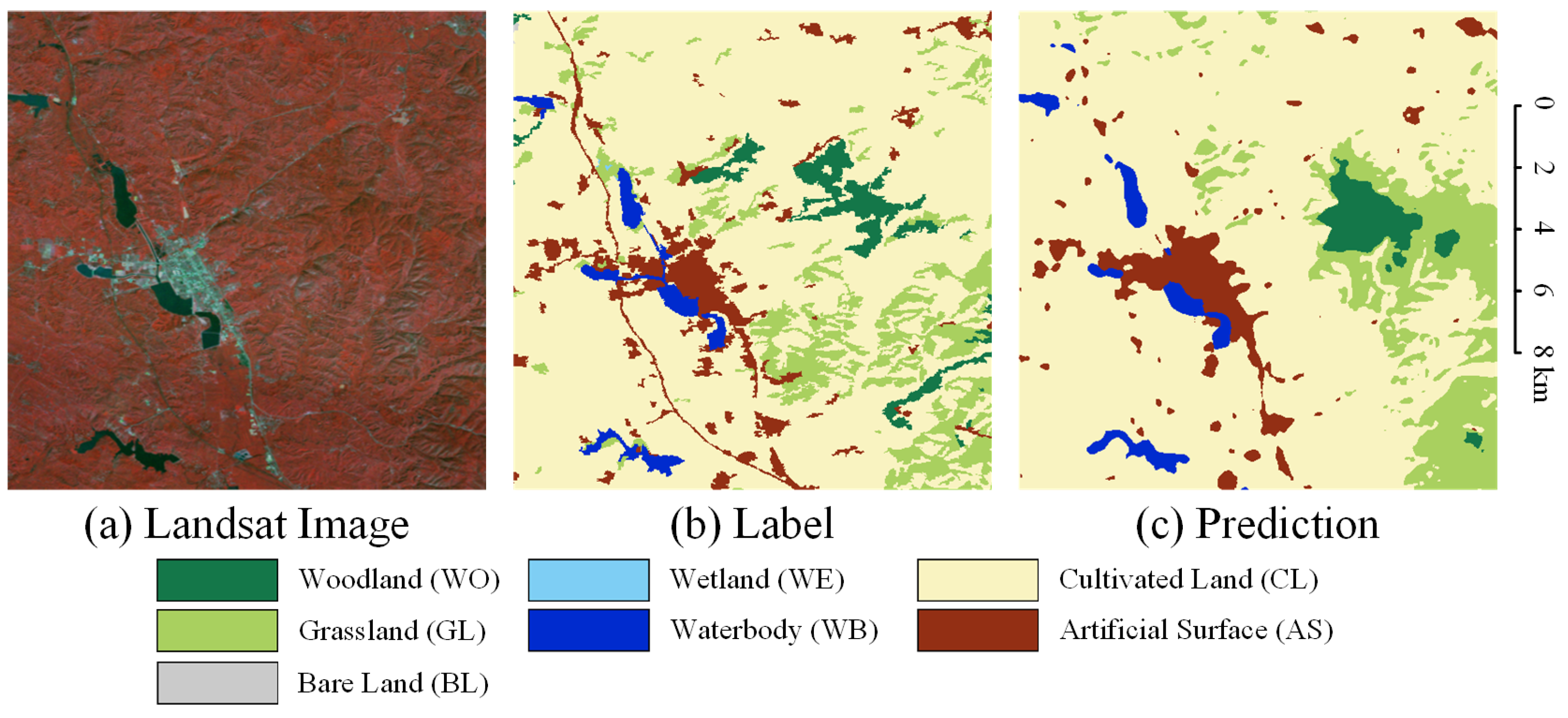


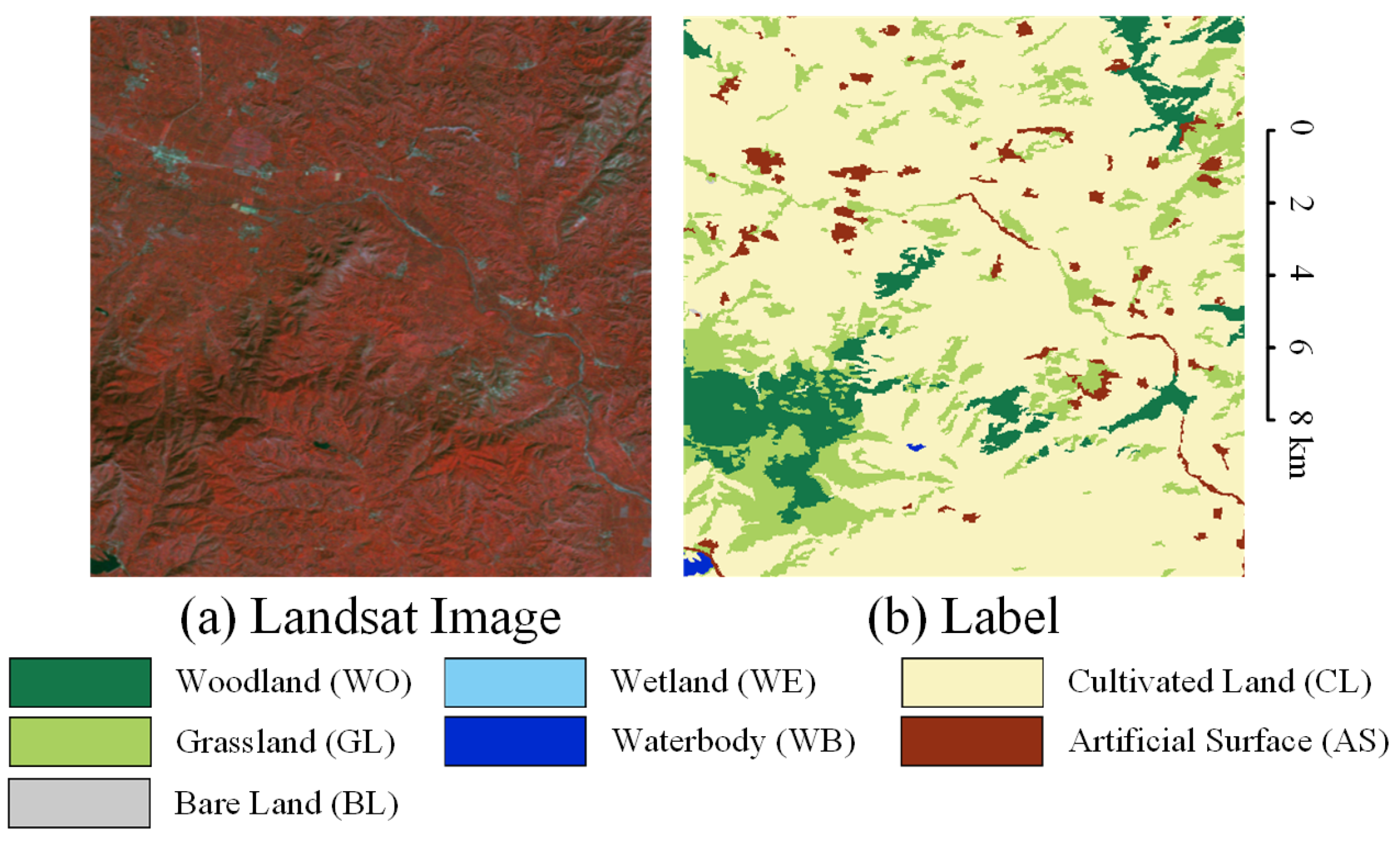
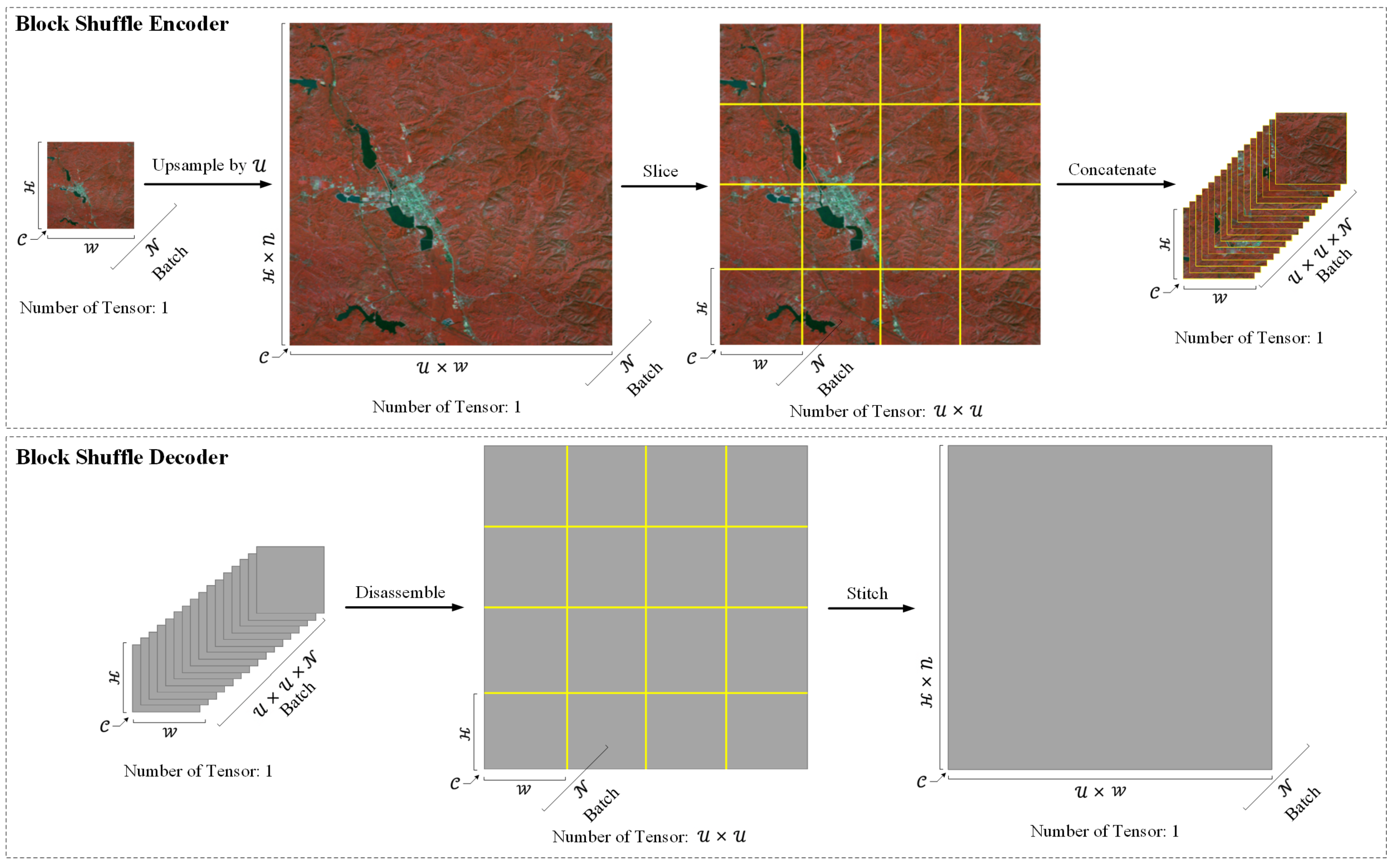
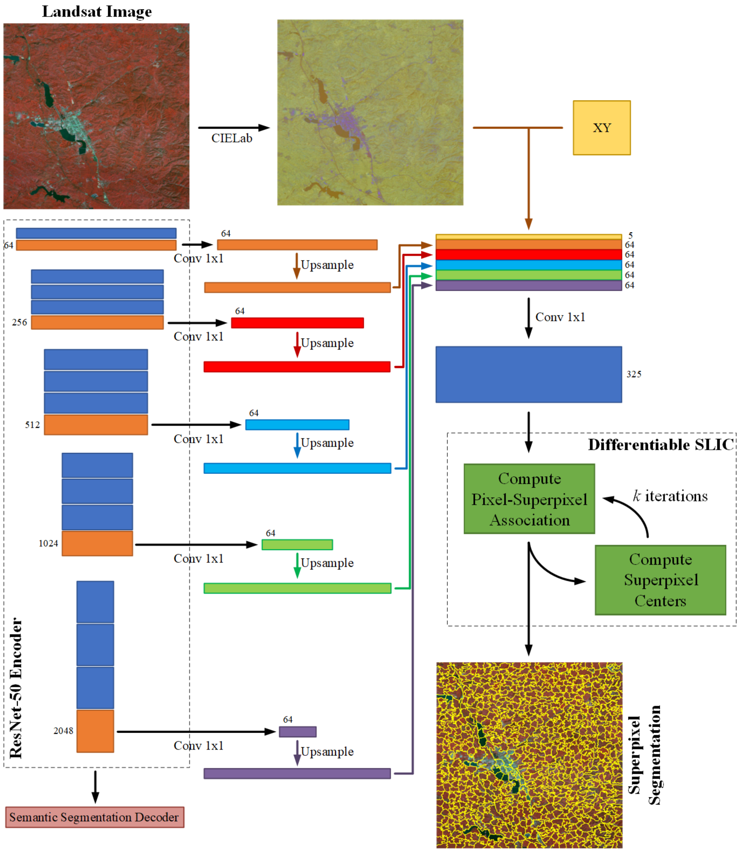
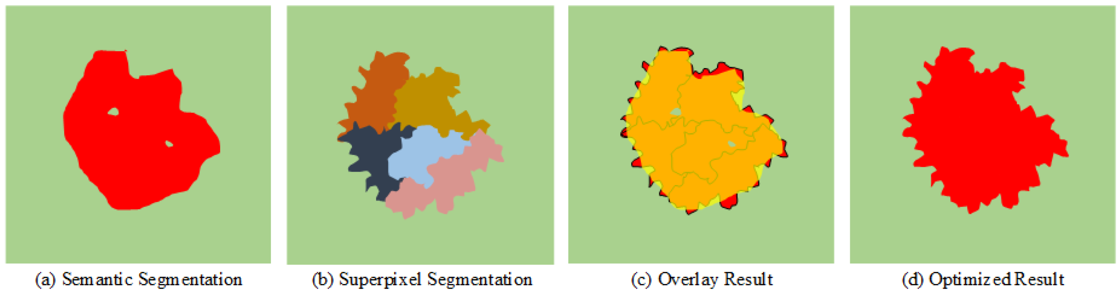
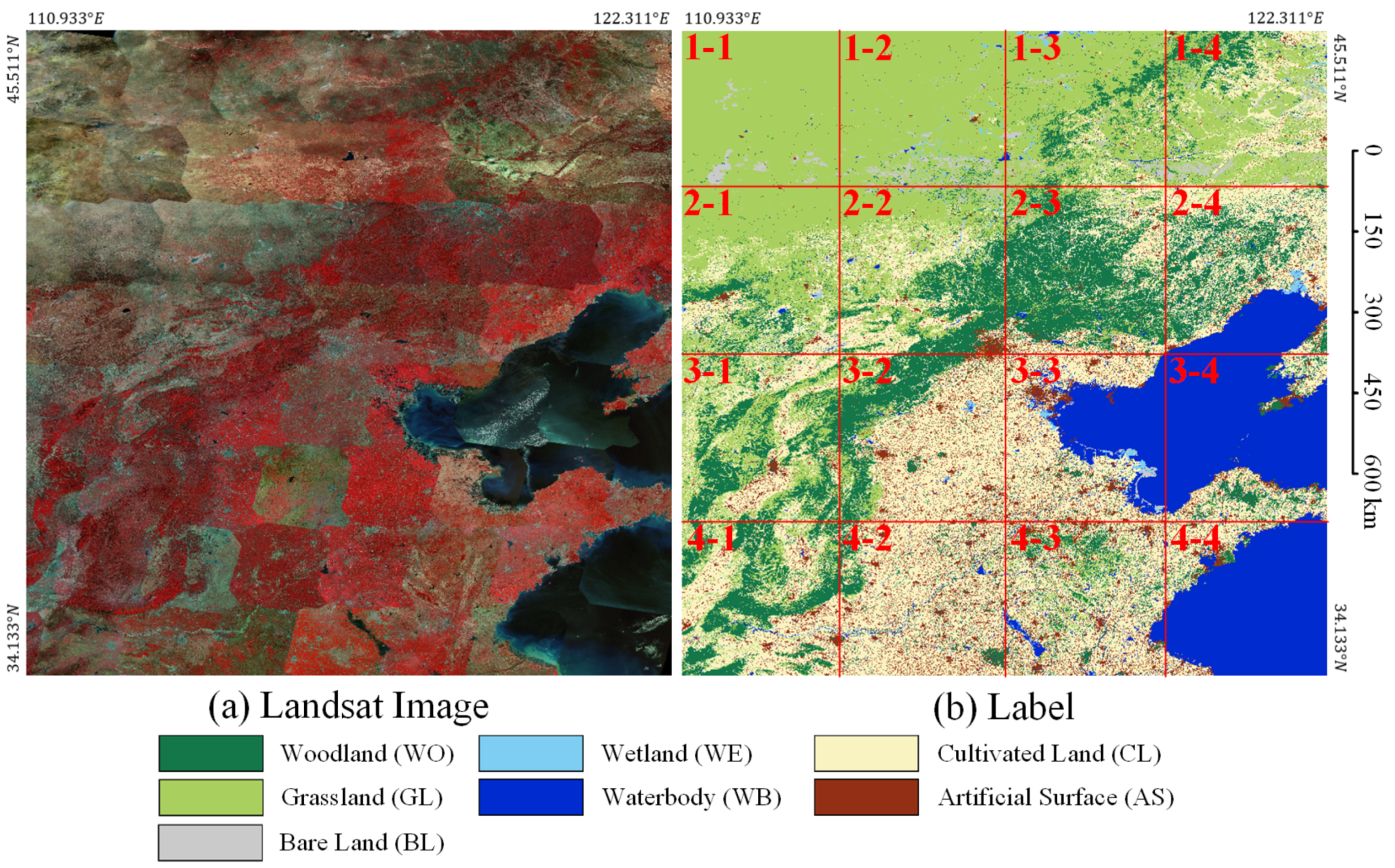

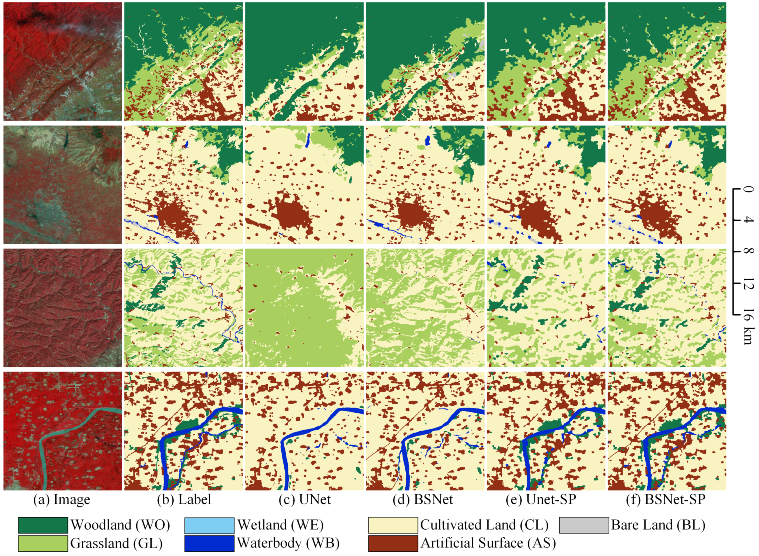
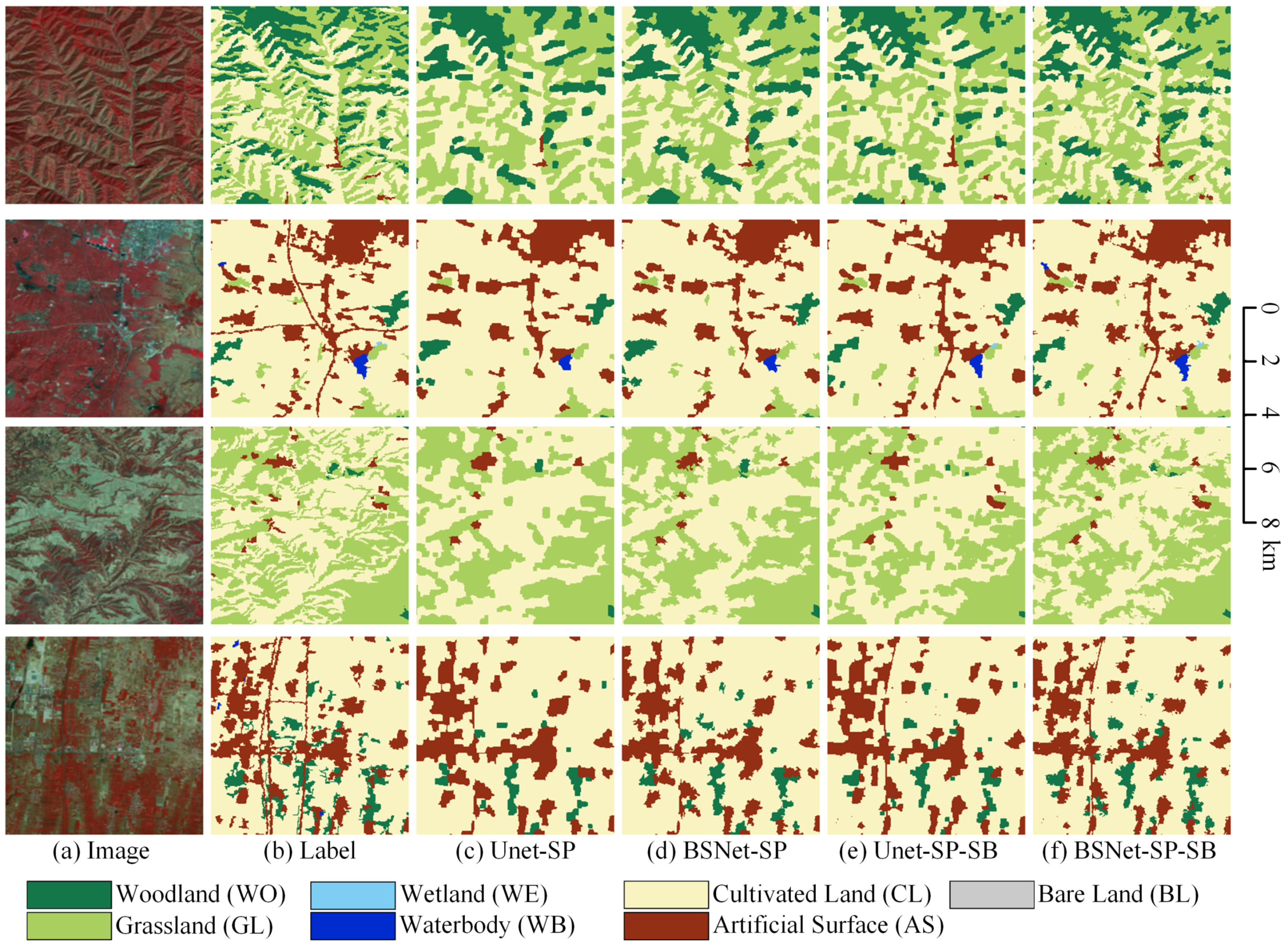
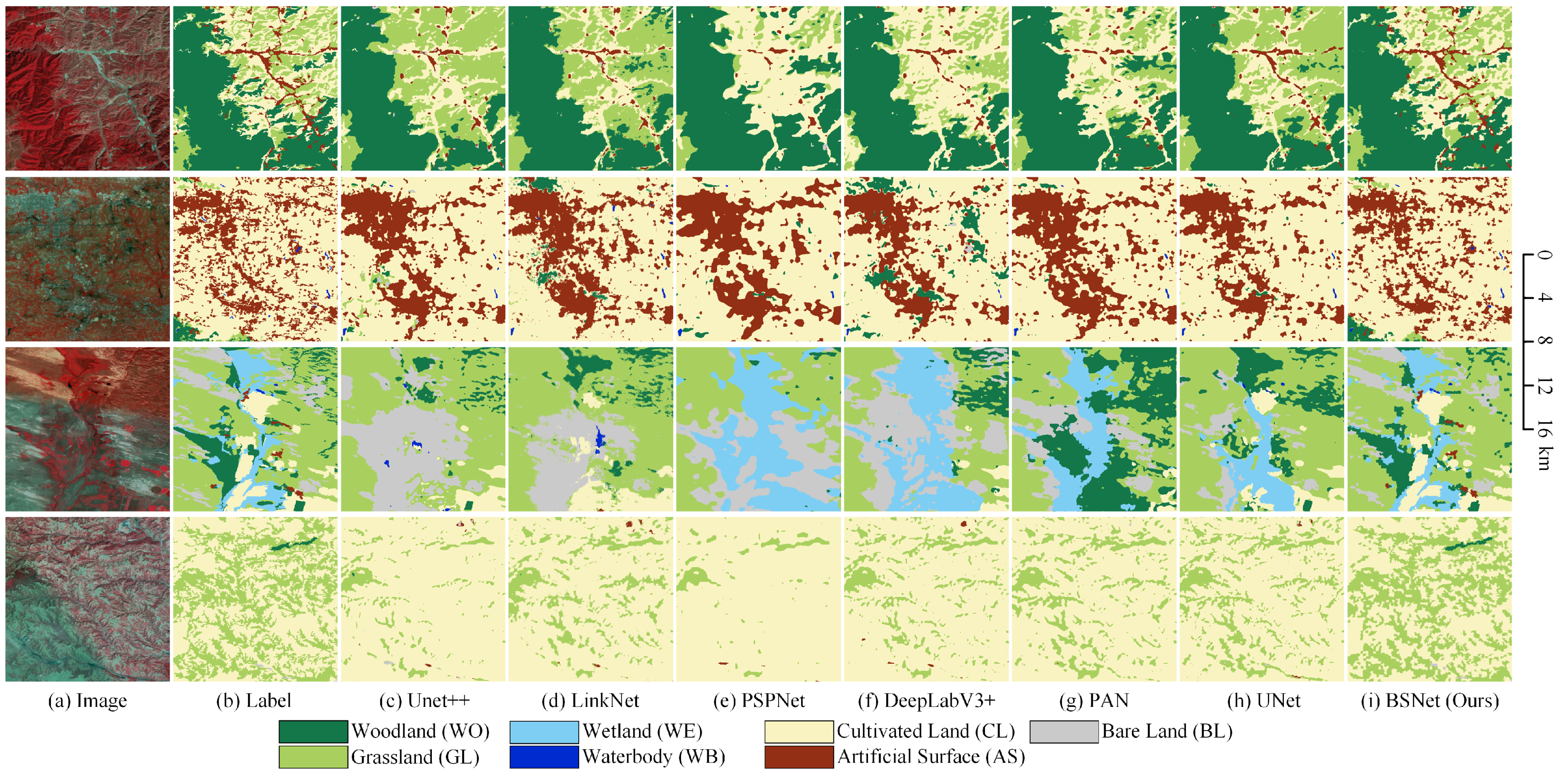

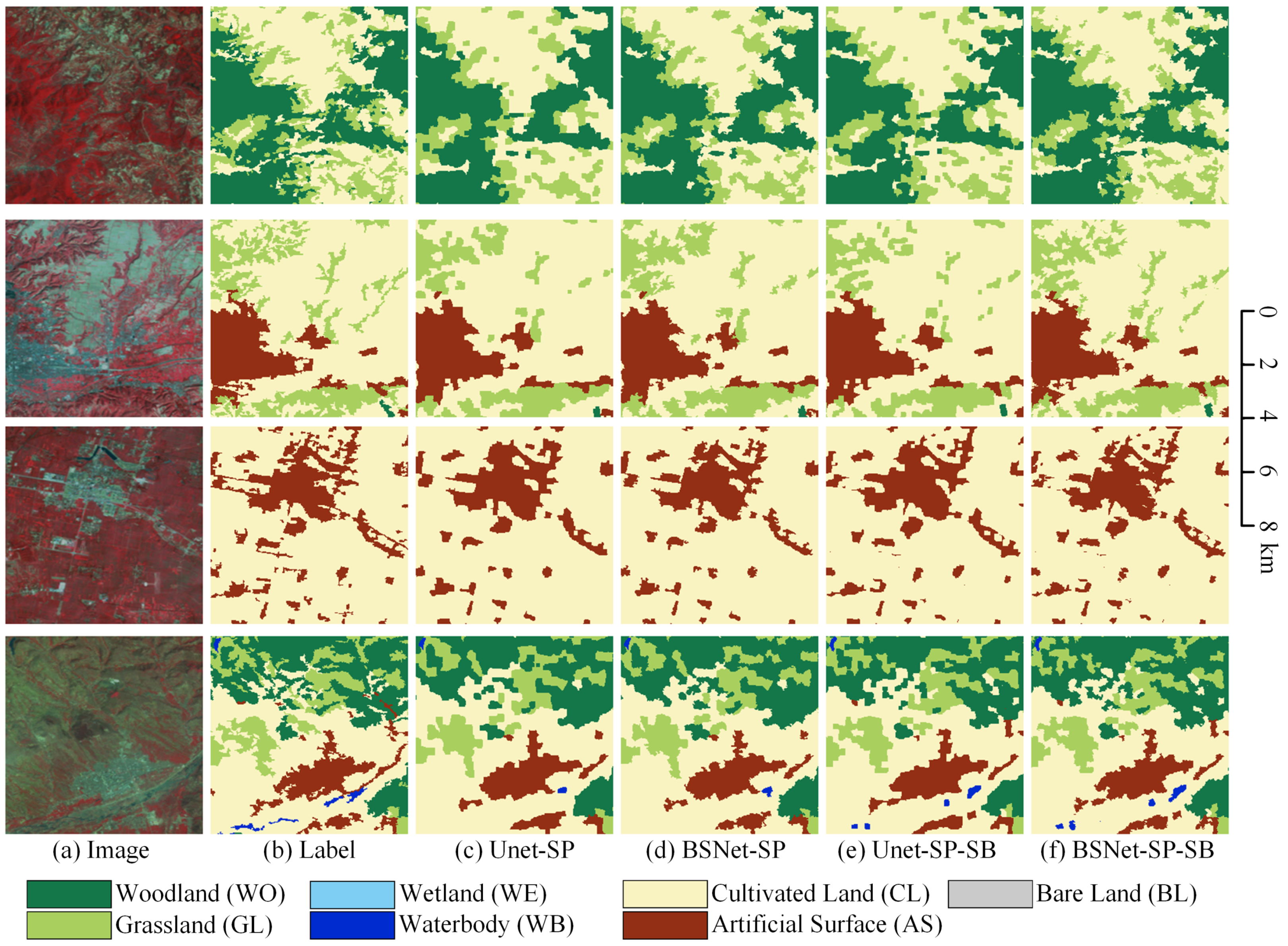
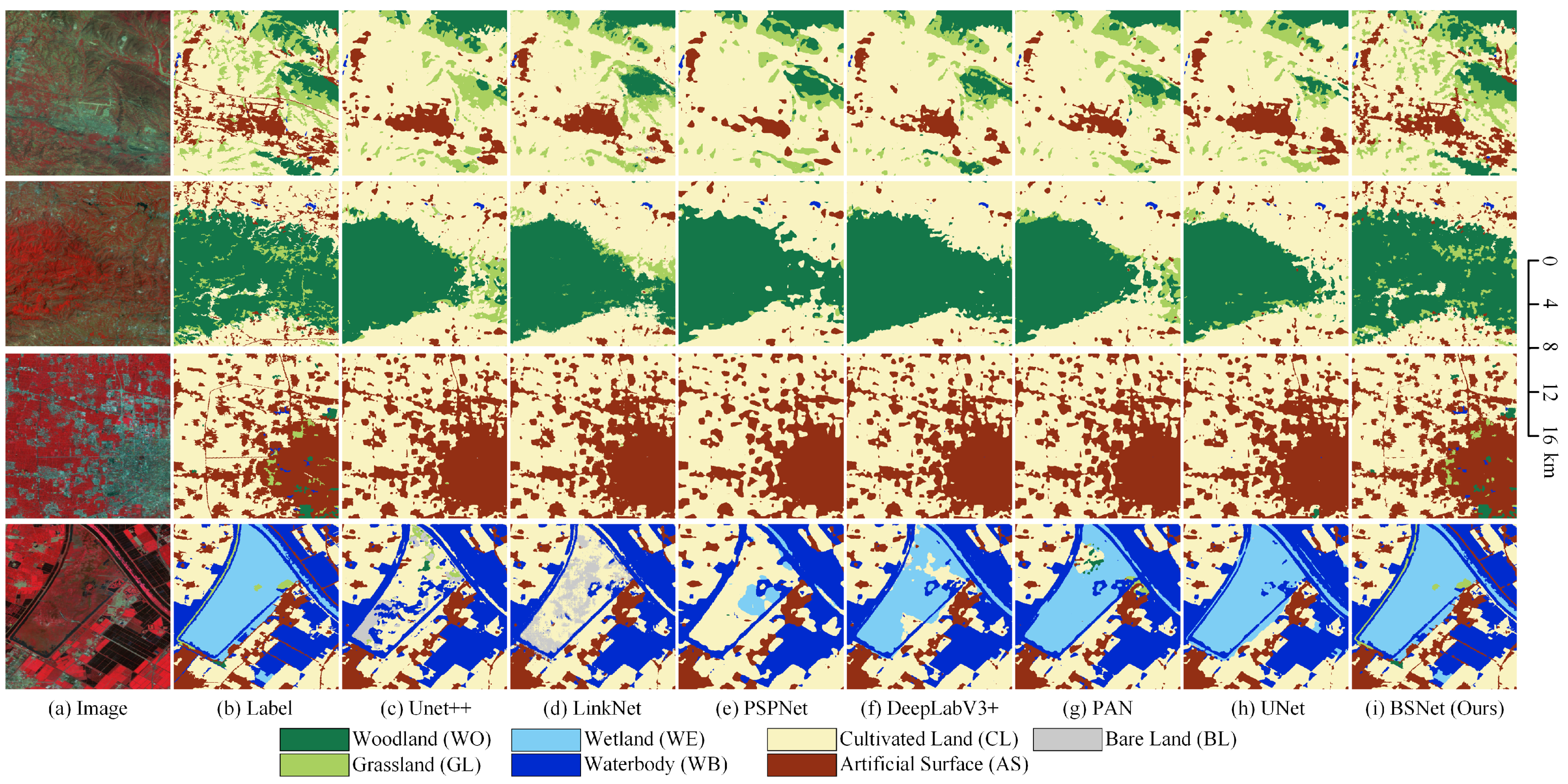
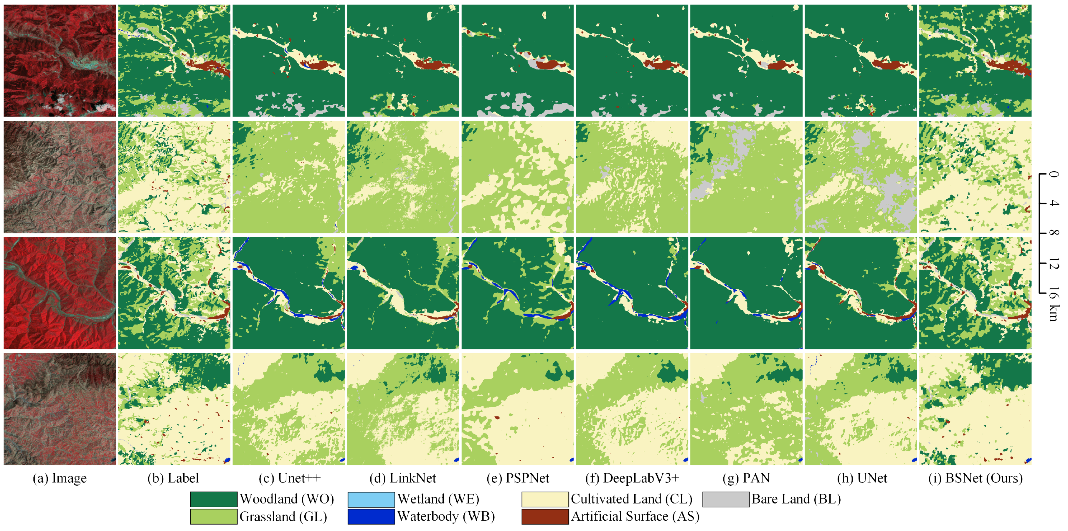

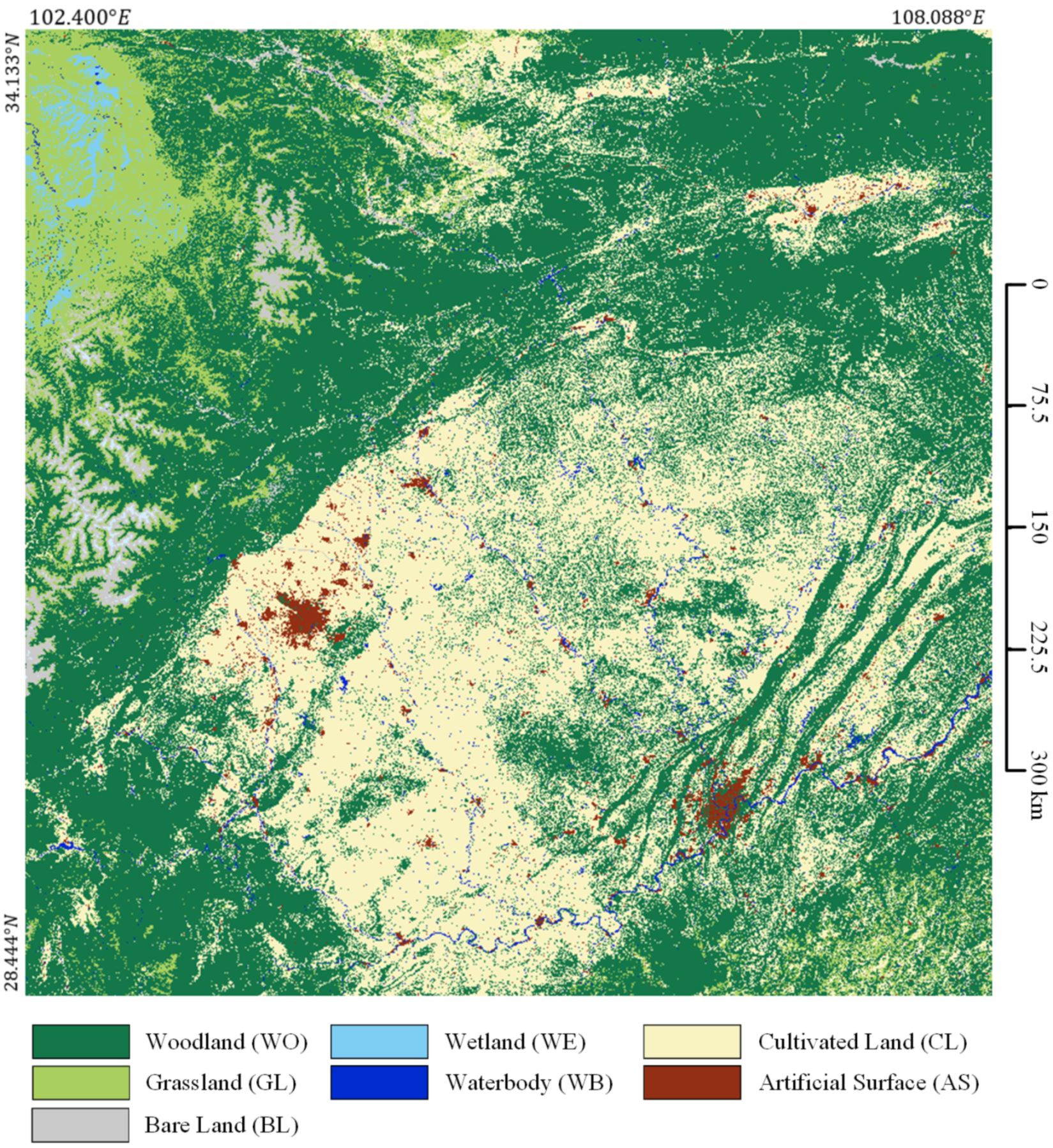
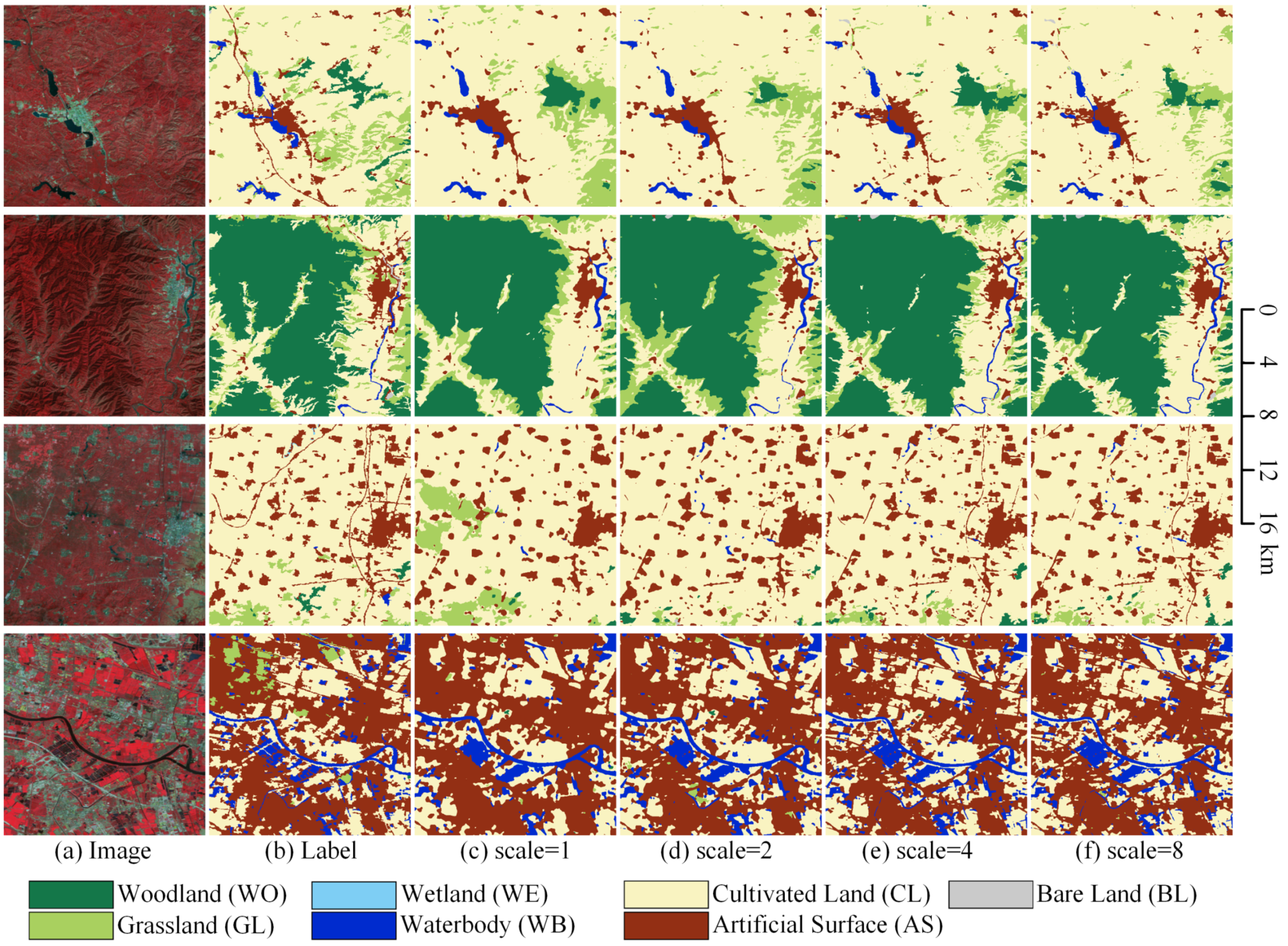
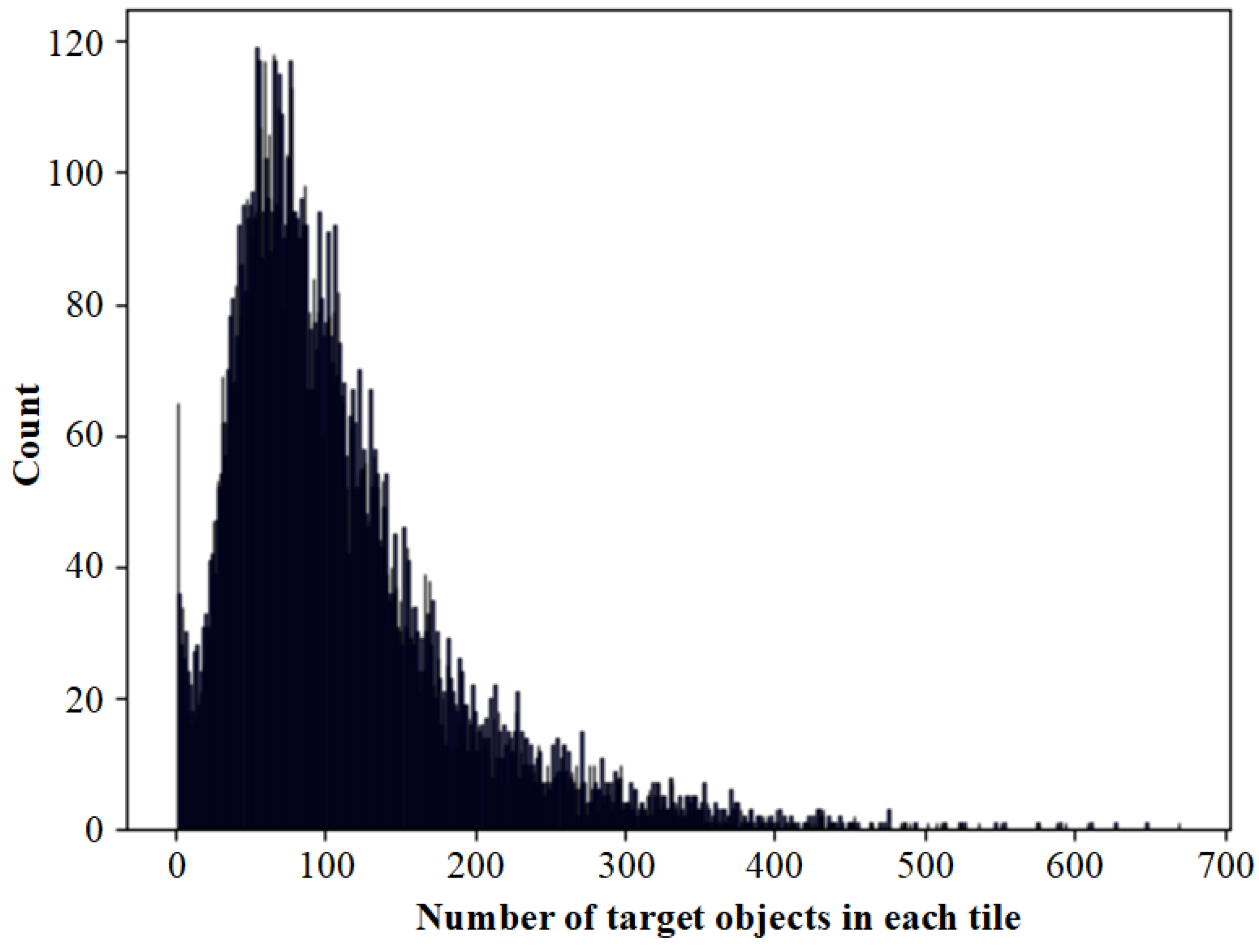
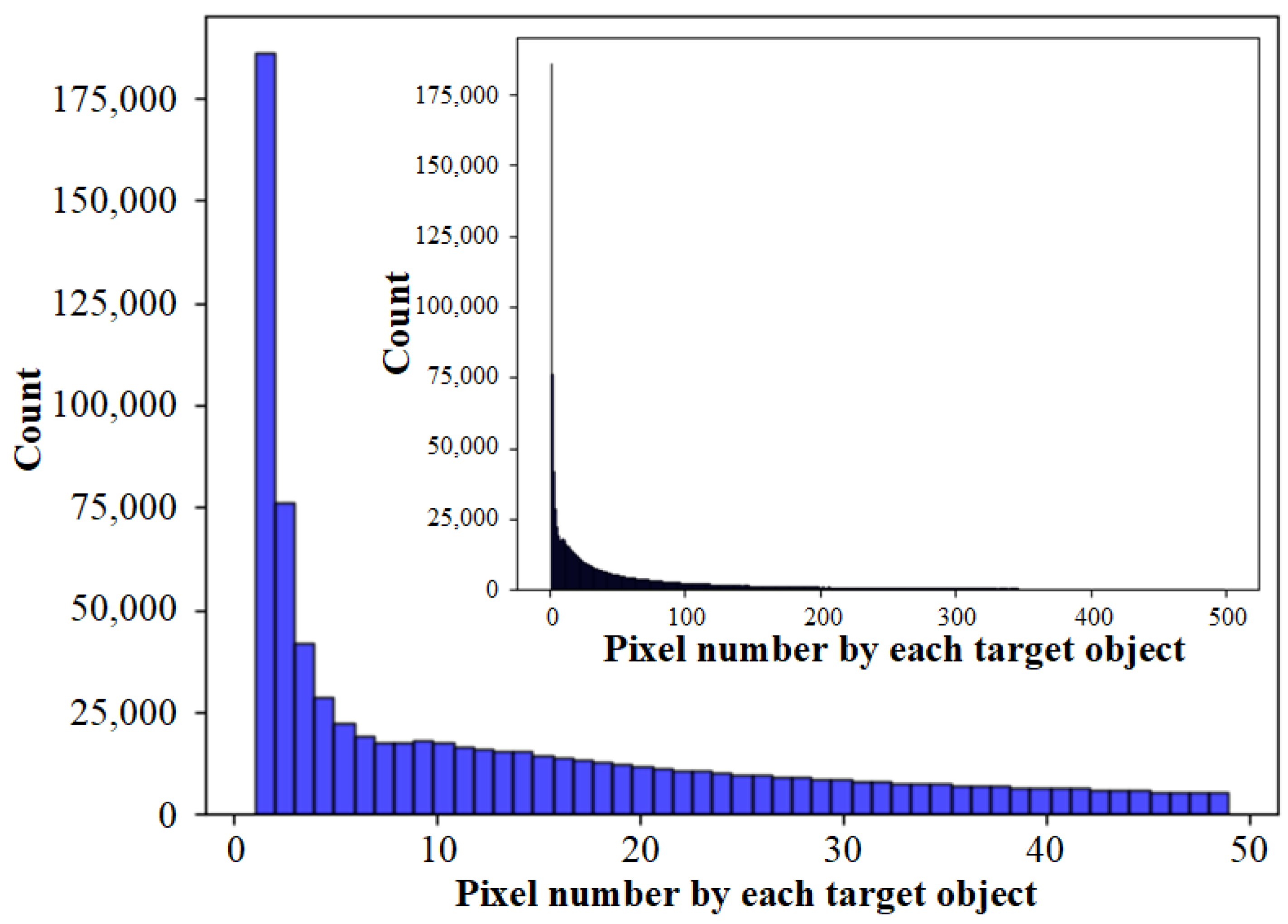
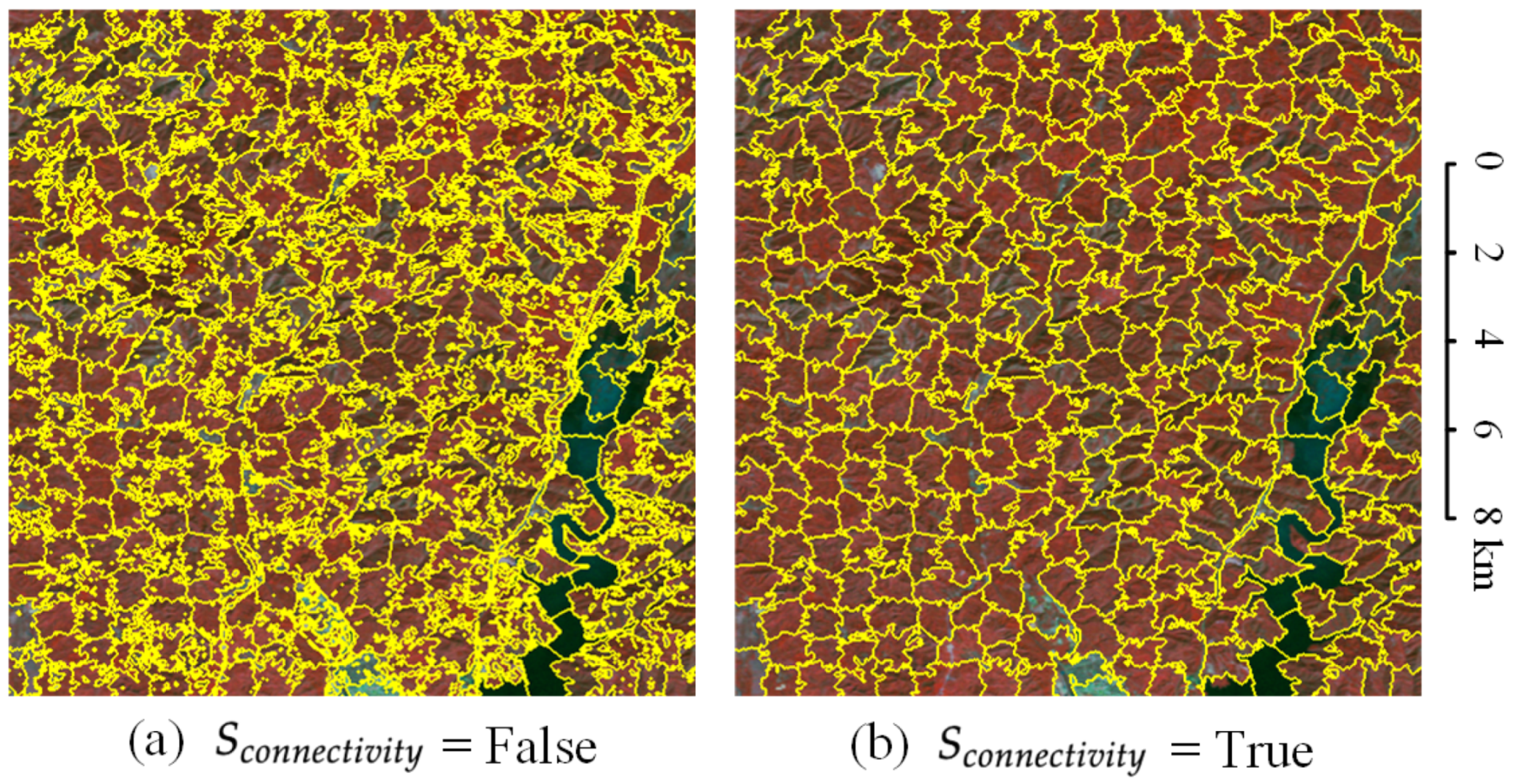
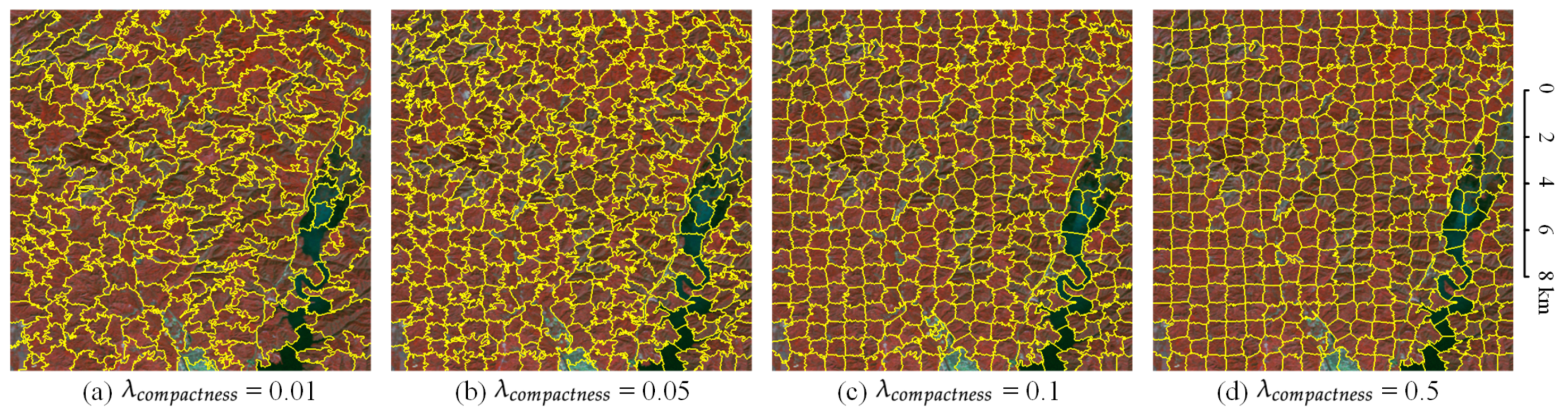
Publisher’s Note: MDPI stays neutral with regard to jurisdictional claims in published maps and institutional affiliations. |
© 2022 by the authors. Licensee MDPI, Basel, Switzerland. This article is an open access article distributed under the terms and conditions of the Creative Commons Attribution (CC BY) license (https://creativecommons.org/licenses/by/4.0/).