Abstract
Discriminative feature learning is the key to remote sensing scene classification. Previous research has found that most of the existing convolutional neural networks (CNN) focus on the global semantic features and ignore shallower features (low-level and middle-level features). This study proposes a novel Lie Group deep learning model for remote sensing scene classification to solve the above-mentioned challenges. Firstly, we extract shallower and higher-level features from images based on Lie Group machine learning (LGML) and deep learning to improve the feature representation ability of the model. In addition, a parallel dilated convolution, a kernel decomposition, and a Lie Group kernel function are adopted to reduce the model’s parameters to prevent model degradation and over-fitting caused by the deepening of the model. Then, the spatial attention mechanism can enhance local semantic features and suppress irrelevant feature information. Finally, feature-level fusion is adopted to reduce redundant features and improve computational performance, and cross-entropy loss function based on label smoothing is used to improve the classification accuracy of the model. Comparative experiments on three public and challenging large-scale remote-sensing datasets show that our model improves the discriminative ability of features and achieves competitive accuracy against other state-of-the-art methods.
1. Introduction
Remote sensing images are a valuable data source and the basis for Earth exploration and observation [1]. With the rapid development of remote sensing satellites and technologies, a large number of spectral- and spatial-information-rich Earth observation images can be obtained by airborne or spaceborne sensors, namely, high-resolution remote-sensing images (HRRSI). These HRRSIs can help us better observe and measure the detailed structure of Earth’s surface. It is particularly urgent to make full use of the ever-increasing HRRSIs for intelligent Earth observation [2]; therefore, it is extremely important to effectively interpret the large and complex HRRSI.
As one of the most representative research areas in HRRSI interpretation, the scene classification of remote sensing images is also an active research field. Scene classification of remote sensing images aims to classify HRRSI into various semantic categories [1]. In recent years, it has attracted a lot of attention [3], and is widely used in geospatial target detection [4,5], natural hazards detection [6], urban planning [7], and especially remote-sensing image interpretation [1].
Compared to ground-scene target classification, the scene classification of remote sensing images is still a challenging research topic due to the following characteristics:
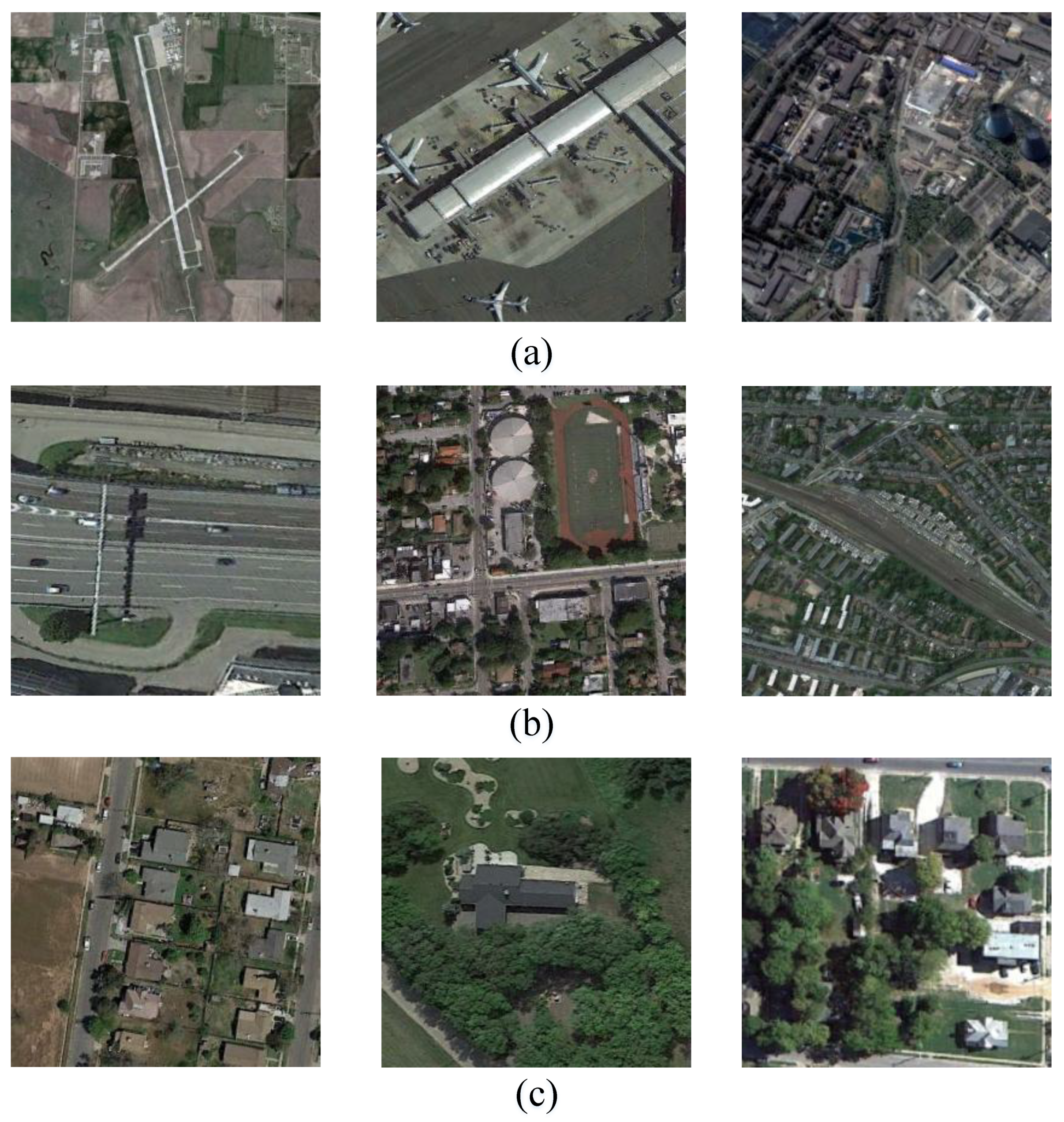
- Large variance in object/scene scales: In remote sensing imaging, different sensors in different platforms work at different altitudes. However, different sensors on the same platform work at the same altitude [8]. With the examples illustrated in Figure 1a, the scenes of airplanes, airports, and thermal power stations have huge scale differences at different imaging altitudes and contain a lot of useless background information. Previous research has shown that deeper network models can be used to extract more valuable feature information [9];
- The complex spatial arrangement, object distribution, and the coexistence of multiple ground objects: As the spatial distribution and arrangement of ground objects are complex and diverse, and remote sensing imaging equipment has a wide bird-eye perspective, it is quite common to include multiple ground objects in HRRSIs. HRRSIs are filled with many key objects, which makes it even more difficult to classify scenarios. As shown in Figure 1b, the scenes of freeways contain trees, cars, bridges, etc. The scenes of ground track fields include roads, swimming pools, and trees. Possible solutions include enhanced local semantic representation of scenarios [9] and approaches that are robust to changes in direction are usually appropriate [10];
- High interclass similarity. The existence of the same object between different scenarios or the high semantic overlap between scene categories results in between-class similarity, which can be extremely difficult to distinguish between these scenes. For example, in Figure 1c, sparse residential, medium residential, and dense residential areas all contain the same ground objects, namely, houses and trees. The bridge and overpass scenarios also contain the same ground object, namely, bridges. Recent studies have shown that although deep convolutional features are utilized for semantic feature representation, the fusion of shallower (low-level and middle-level features) can make features more discriminative [11,12].
With the rapid development of deep learning, scholars have proposed many convolutional neural network models (CNN), such as LGRIN [12]. Some improved networks have also achieved state-of-the-art performance [10,12,13]. The success of CNN models demonstrates that high-level features can be used to describe scenes better than low-level and middle-level features [14,15]. Nevertheless, the following problems remain:
- Loss of shallower features (low-level and middle-level features): Commonly used CNN models cannot preserve shallower features during the training process [8]. In addition, when CNN models go deeper, models tend to lose shallower features [16]. However, these shallower features help to enhance the ability of scene representation and improve the accuracy of classification. Some recently proposed approaches for preserving shallower features are not end-to-end [15,17], as it is difficult to adapt to different application scenarios;
- Lack of local semantic features: Since most CNN models utilize the last connection layer as the global feature representation to complete scene classification [18,19], the local regional features of images are ignored. Two remote sensing images with different global structures may belong to the same category because they contain some obvious and same target objects [20]. However, some models only use global semantics to discriminate, which will reduce the accuracy of classification [9];
- Insufficient consideration is given to the correlation between features: Since a certain feature tends to represent the image from one aspect and ignores other feature information, complementary features are usually used to make up for the missing features [21,22,23]. However, how to select and represent features is still one of the main research topics in the field of machine learning. Serial features and parallel features are two typical methods [24]. However, these methods do not fully consider the correlation between features, leading to feature redundancy, increasing the complexity of calculation, and are not very effective for scene classification.

Figure 1.
Challenges of HRRSI: (a) large variance in object/scene scales; (b) complex spatial arrangement, object distribution, and the coexistence of multiple ground objects; (c) high interclass similarity. The images are from the NWPU dataset [25].
Figure 1.
Challenges of HRRSI: (a) large variance in object/scene scales; (b) complex spatial arrangement, object distribution, and the coexistence of multiple ground objects; (c) high interclass similarity. The images are from the NWPU dataset [25].
To address the above problems, in this study, we propose a novel Lie Group deep learning model based on attention mechanisms. The goals include the following.
- Preserve shallower features: Most CNN models cannot preserve shallower features. In addition, the existing methods for preserving shallower features are not flexible end-to-end frameworks [15,17]. Our model involves an end-to-end network to preserve the features of different levels (low-level, middle-level, and high-level) and effectively improve the classification accuracy of the model;
- Enhance local semantic features: Most existing CNN models usually combine local domain filters (average or maximum feature value), which limits the representation of local semantics [25,26,27]. Our model should have the ability to improve the representation of key features;
- Enhance feature representation and improve computing performance: Although some methods utilize both local and global features as the final representation [10], they do not consider the interrelation between different features in the HRRSIs. Therefore, our model should consider the relationship between different features and reduce the parameters of the model to improve the computational performance and ensure effective HRRSI feature extraction.
The main contributions of this paper are as follows:
- A novel efficient HRRSI scene classification model: The Lie Group deep learning (LGDL) model based on an attention mechanism can effectively improve the ability of scene feature representation, the accuracy of scene classification, and can better classify complex scenes. Considering the characteristics of HRRSIs, LGDL utilizes Lie Group machine learning (LGML) to preserve the shallower features (low-level and middle-level features) of HRRSIs, such as scale-invariant feature transform (SIFT) [28] and local binary patterns (LBP) [29]. In addition, deep learning is used to extract high-level semantic features of HRRSI. Finally, automatic scene learning is implemented based on the fused multi-source heterogeneous features;
- The spatial attention mechanism is used to suppress the weight of irrelevant feature information to improve the ability of local key semantic features. Compared with the maximum pooling and mean operation used in the traditional model, our method improves and enhances the ability of local semantic representation. To deal with HRRSIs in complex scenes, we utilize parallel dilated convolution to enrich scale feature information and utilize kernel decomposition to increase the number of skip connections and reduce the difficulty of training deeper models;
- The Lie Group covariance feature matrix is introduced to represent the extracted shallower features. The feature matrix is a real symmetric matrix, which fully considers the correlation between shallower features and has good computing performance and anti-noise ability. Features of different levels (low-level, middle-level, and high-level) and different spaces are integrated through efficient feature-level fusion. This method fully considers the correlation between features of different layers, avoids feature redundancy and reduces feature dimension, enhances the feature representation ability, and maintains a good computing performance.
The rest of this paper is arranged as follows. Section 2 outlines the existing literature related to scene classification, LGML, and the attention mechanism. Section 3 describes our proposed model in detail. Section 4 evaluates the proposed model against various state-of-the-art models on three public and challenging scene datasets and performs ablation experiments. Finally, conclusions are provided in Section 5.
2. Related Work
In this section, we review some related works of scene classification, LGML, and attention mechanisms.
2.1. Scene Classification Methods
From the perspective of feature extraction and learning, remote sensing scene classification methods are mainly divided into low-level, middle-level, and high-level feature methods. It is worth noting that these three feature methods are not necessarily independent of each other.
2.1.1. Methods Based on Low-Level Features
In the early stage of remote sensing scene classification, scholars extracted a series of low-level features according to the characteristics of remote sensing images, such as SIFT [28], LBP [29], and color histograms (CH) [30]. In fact, the above features are not independent of each other, and the fusion of various features has achieved good results in remote sensing scene classification [31]. However, the above features rely heavily on the prior knowledge of experts [20]. It is difficult for them to achieve optimum performance in complex scenarios.
2.1.2. Methods Based on Middle-Level Features
To address the shortcomings of the low-level feature method, scholars have proposed a method based on middle-level features, which encoded the above features to obtain higher-order statistical mode, extract more important features in the image, and establish global representation. Typical methods are bag-of-visual-words (BoVW) [32] and probabilistic topic models (PTM) [33] (i.e., probabilistic latent semantic analysis (PLSA) [34] and latent Dirichlet allocation (LDA) [33]). However, this method also has shortcomings: It ignores the correlation between features [35,36], and the feature selection and design also rely on expert domain knowledge, etc.
2.1.3. Methods Based on High-Level Features
In recent years, the deep learning model has profoundly improved the performance of remote sensing scene classification [37,38,39,40,41]. Typical models include CNNs [42], generative adversarial networks (GAN) [43], and autoencoders [44]. Compared with the above two methods, the deep learning model can extract more high-level features and obtain better classification performance [12,45]. This kind of deep learning model usually adopts an autonomous learning feature of a multi-layer network structure and regards the remote sensing scene classification as an end-to-end problem [46].
2.2. Lie Group Machine Learning (LGML)
LGML is a novel branch of the machine learning knowledge system, which has the advantage of a manifold structure and forms a new learning paradigm based on the idea of Lie Groups [47]. Xu et al. [20] proposed a new algorithm based on Lie Group intrinsic mean, deduced the Lie Group kernel function, which can be applied to both matrix and vector data samples, and achieved good results in remote sensing scene datasets. Later, Xu et al. [48] improved the algorithm to further improve the classification accuracy of the model and reduce the number of parameters of the model. Xu et al. [12] proposed a novel scene classification model jointly represented by Lie Group and CNN, which further improved the accuracy of scene classification and the interpretability of the model from the perspective of LGML. Compared with traditional methods, the LGML method does not lose too much image information. Lin et al. [49] utilized the Lie Group Lie Algebra method in the affine transformation process and verified the robustness of the LGML method to direction change. In addition, the LGML method is also used in target recognition detection [50] and pedestrian detection in the video [51], both of which have achieved good results. Tran et al. [52] used automobile point cloud to construct Lie Group samples and used principal geodesic analysis (PGA) [53] to design classifiers, whose classification effect is significantly better than traditional linear methods [54]. Therefore, the LGML method has good advantages in image affine transformation modeling, feature representation, and classification.
2.3. Attention Mechanism
The attention module is designed to focus on the most important part of features. It is inspired by the human perception process [55], and it is an algorithm that simulates human understanding and the perception of images, and can effectively suppress irrelevant feature information. Woo et al. [56] proposed a convolutional block attention module (CBAM), which weighted attention in spatial and channel dimensions, enabling the model to effectively learn key features in the image and improve the performance of most models. Hu et al. [57] fused key points with salient regional features to complete scene classification. Zhang et al. [58] used a significance sampling strategy to extract key features in remote sensing images for classification. However, the above saliency detection method based on texture feature information cannot effectively extract all key feature information. Recently, an adaptive method for extracting key attention features has been proposed. Mnih et al. [59] combined the recurrent neural network model with the attention mechanism to reduce the feature dimension. Haut et al. [60] used the generated attention masks to multiply the corresponding regions to obtain attention features. Xu et al. [61] proposed an image task model based on “soft“ and “hard“ attention, which is trained by different propagation algorithms. Hu et al. [62] proposed a squeeze-and-excitation module, which utilizes the global average pooling to abstract the internal features and calculates the weight of each feature through nonlinear activation and linear combination.
3. Method
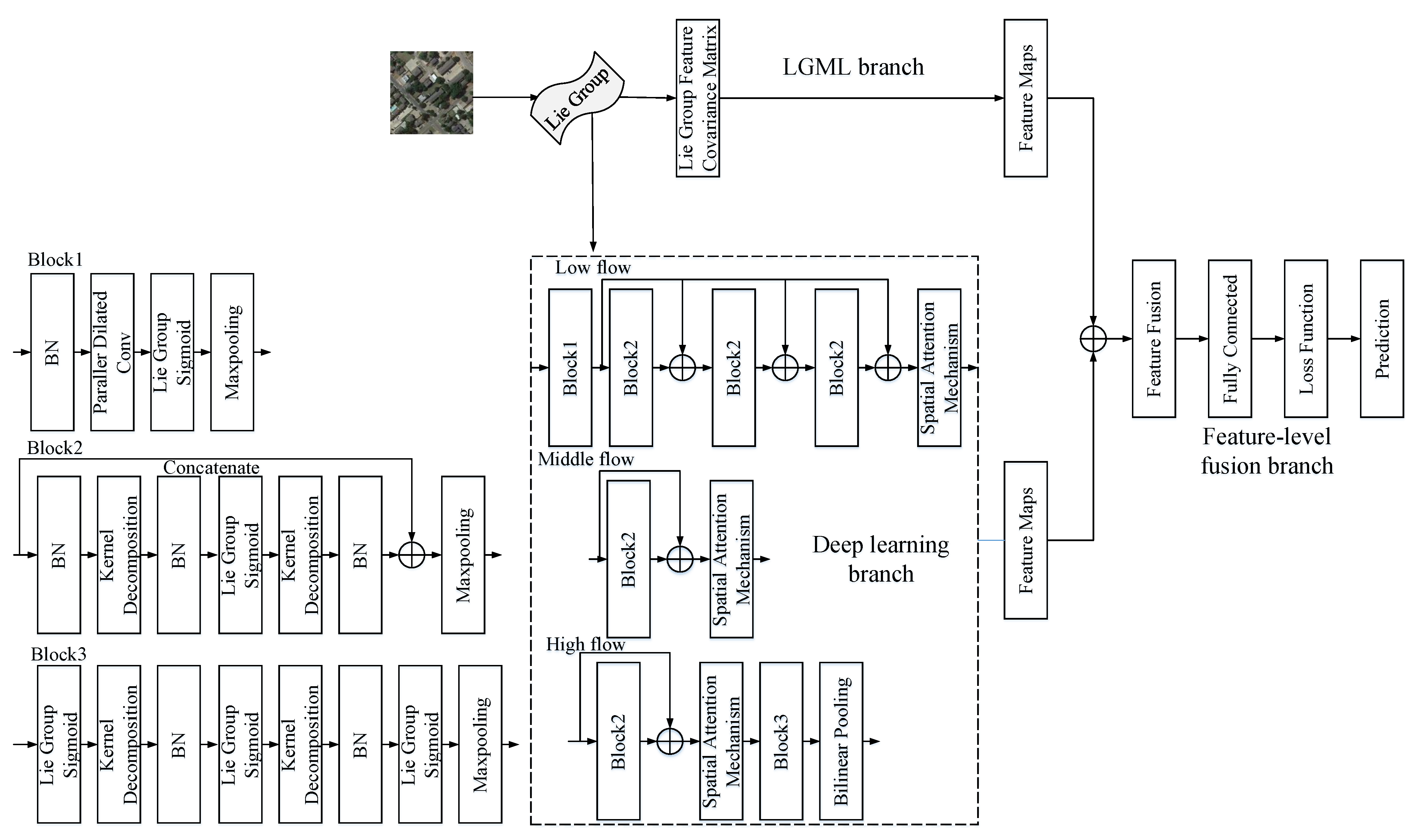
In this section, the LGDL model is carefully designed to improve the scene classification performance of HRRSI. As shown in Figure 2, the model mainly consists of three branches: LGML branch, deep learning branch, and feature-level fusion branch. For the branch of LGML, the HRRSI extracts shallower features through LGML and implements feature representation through the Lie Group feature covariance matrix. For the branch of deep learning, this branch is divided into three parts: (1) Low flow, (2) Middle flow, and (3) High flow. This branch is used to extract high-level features. Finally, the features extracted from the above two branches are transferred to the feature-level fusion branch, and the improved cross-entropy loss function is used to make the final prediction after the feature-level fusion is completed. By combining the above branches, the feature discrimination of our proposed model is enhanced, the parameters of the model are reduced, and the computational performance of the model is improved. The three branches of our model will be elaborated separately.
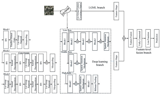
Figure 2.
Architecture of our proposed model. The model includes (1) LGML: used to extract shallower features; (2) Deep learning branch: used to extract high-level features; (3) Feature-level fusion branch: used to fuse features.
3.1. LGML Branch
In the task of pattern recognition, it is a key and significant step to extract the discriminative features from data. Remote sensing scene classification is no exception. During the past decade, scholars have been devoted to design discriminative features, as it is critical for remote sensing scene classification, especially for some scenes that do not contain objects, such as forests, beaches, and deserts. For these scenarios, the low-level and middle-level features are more discriminative than the high-level features. Inspired by this, in this section, we extract the low-level and middle-level features of the scene and use the Lie Group feature covariance matrix to represent them.
3.1.1. Sample Mapping
To make full use of the computational advantages and manifold space structure of Lie Groups and Lie Algebras, firstly, we map the data samples to Lie Group manifold space:
where represents the jth sample of the ith class in the dataset, and represents the jth sample of the ith class in the manifold space of the Lie Group. The following operations are based on the Lie Group data sample [12].
3.1.2. Lie Group Feature Covariance Matrix
According to the above analysis, to enhance the feature representation ability of different scenes, the following features are utilized:
where represents the pixel position; represent the brightness, color difference, and saturation of space, respectively; and represent the first-order gradient and the second-order gradient at the coordinate position , respectively. The above three features are the most basic feature information of the target object. The same scene contains similar target objects, although these target objects are different in size and shape, their positions in the scene are similar, and the rate of change of pixels is similar. Colors are extremely discriminating features, such as white clouds, blue oceans, and green forests. However, it is not enough to utilize a single color feature. To enhance the robustness and stability of the feature, we choose . Experiments have proven that these features have better robustness and stability to scene transformation [12,50,63].
[64,65] represents the grayscale image of the scene, which can simulate the single-cell receptive field of the cerebral cortex to extract significant features. [12,65] refers to the binarization operation of the surrounding pixels, which can effectively extract the texture features of ground objects and is invariant to monotonous illumination changes. [28] represents gradient information in the image, which is invariant to brightness, scale, and rotation changes. Histogram of Oriented Gradients () [45,66] represents the statistical feature of the gradient direction histogram of the local area of the image, which has rotation invariance, scale invariance, and sparsity.
The feature covariance matrix of Lie Group is a real symmetric matrix, which represents the variance of features in the diagonal line and the relations between features in the non-diagonal line. In addition, this matrix has a lower dimension, is not affected by the size of HRRSI, has anti-noise ability, and has good computing performance. For other detailed information about this feature matrix, please refer to [12,50].
3.2. Deep Learning Branch
In recent years, remote sensing scene classification methods have sprung up, especially the model based on deep learning [1]. Generally, with the deepening of the network model structure, the model can extract deeper features [1]. However, a very deep model is difficult to train from the very beginning, and the model has the following risks [67]: (1) overfitting, (2) model degradation, and (3) a large number of parameters and high computational complexity. To address the risks or problems mentioned above, we utilize parallel dilated convolution, kernel decomposition, and pyramid residual connection operations, as shown in Figure 2.
3.2.1. Batch Normalization (BN)
The goal of this layer is to standardize input sample information by reducing internal covariate shift [68]. Previous studies [68] showed that the BN layer inserted before the convolutional layer could accelerate the convergence speed of the model and effectively improve the structural capability of the model. Therefore, in this study, we adopt this approach.
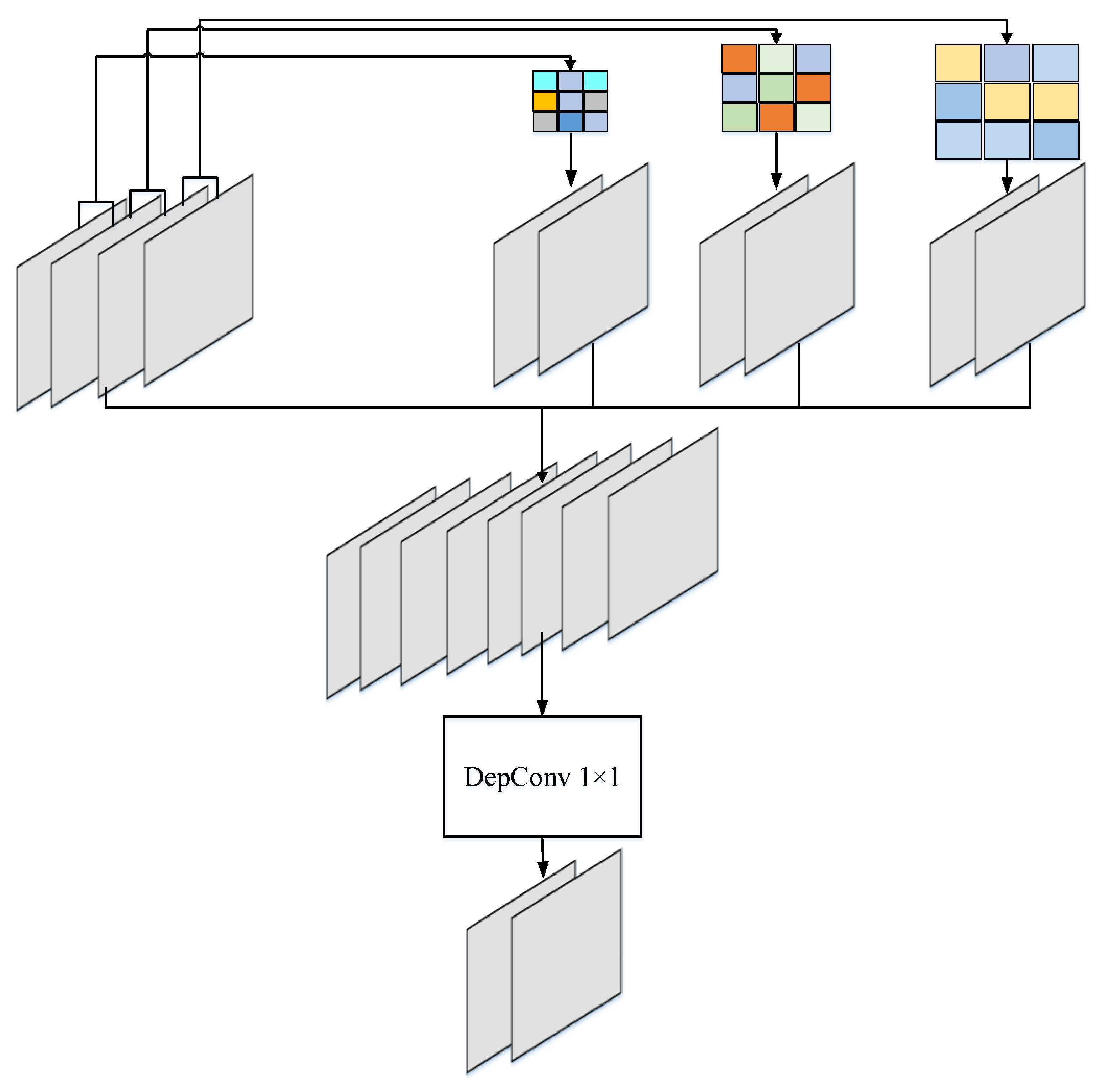
3.2.2. Parallel Dilated Convolution
According to the basis of previous research [12], the existing model adopts depth separable convolutions (DepConv), mainly because the computation of DepConv is eight to nine times less than that of standard convolutions [69], and it contains fewer parameters. However, DepConv does not provide a large enough receptive field for large scenes. Dilated convolution is an effective method to enlarge the receptive field and ensure that large scenes are captured. However, previous studies show that dilated convolution is a time-consuming operation [12,70]. An important goal of our model design is to guarantee good classification accuracy while keeping good computational performance, that is, to expand the receptive field without increasing the computational complexity and the number of parameters of the model.
To address the above problems, three parallel dilated convolution operations with different dilation rates are adopted in this study, as shown in Figure 3. To reduce parameters and make the model more slim, shared weights are adopted for parallel dilated convolution. Assume the feature map and divide it into four parts along the channel , as shown below:
where represents the dilated convolution using the dilation rate , represents the shared parameters, represents the dilated convolution function, and represents the result of concatenating the output of the dilation convolution and the original feature maps. Finally, a depthwise convolution is used to reduce the number of channels:
where represents the final output.
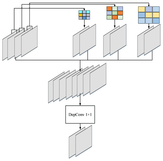
Figure 3.
The principle of parallel dilated convolution. The dilation rates are 2, 4, and 6, respectively.
The above operation merges multi-scale features into . However, in the model, extra features are not always helpful, sometimes increasing the computational complexity of the model and even bringing unexpected consequences. This is another reason why we utilize shared weights. Different dilation rates adopt one filter operation, which is beneficial to the training of the filter and can avoid overfitting to a certain extent. In addition, previous studies have verified that the impact of parallel dilated convolution on time cost is insignificant [70].
As shown in Table 1, the number of parameters of three parallel dilated convolution and ordinary convolution is analyzed. From Table 1, we find that although the kernel size is enlarged, its parameters are much less than those of the other two convolutions. In addition, biases are not used in the module.

Table 1.
The number of parameters of three parallel dilated convolution and ordinary convolution.
3.2.3. Lie Group Kernel Function
In the field of machine learning, a large part of training and test data samples are matrix data samples forms other than the common vector data samples forms. In many existing applications, a large number of matrices constitute Lie Groups [47]. Since the dot product operation of vectors satisfies the commutative law, and matrix multiplication does not satisfy the commutative law, therefore, the traditional kernel function based on the vector cannot be applied to the data sample of the Lie Group matrix. According to the basis of previous studies [20,48], after repeated experimental analysis, the Sigmoid kernel function of Lie Group is adopted in this model:
where represents the trace calculation of the matrix; for other relevant parameters, please refer to [20,48]. The Lie Group kernel function can satisfy both matrix data samples and vector data samples, which enhances the universality and robustness of the model.
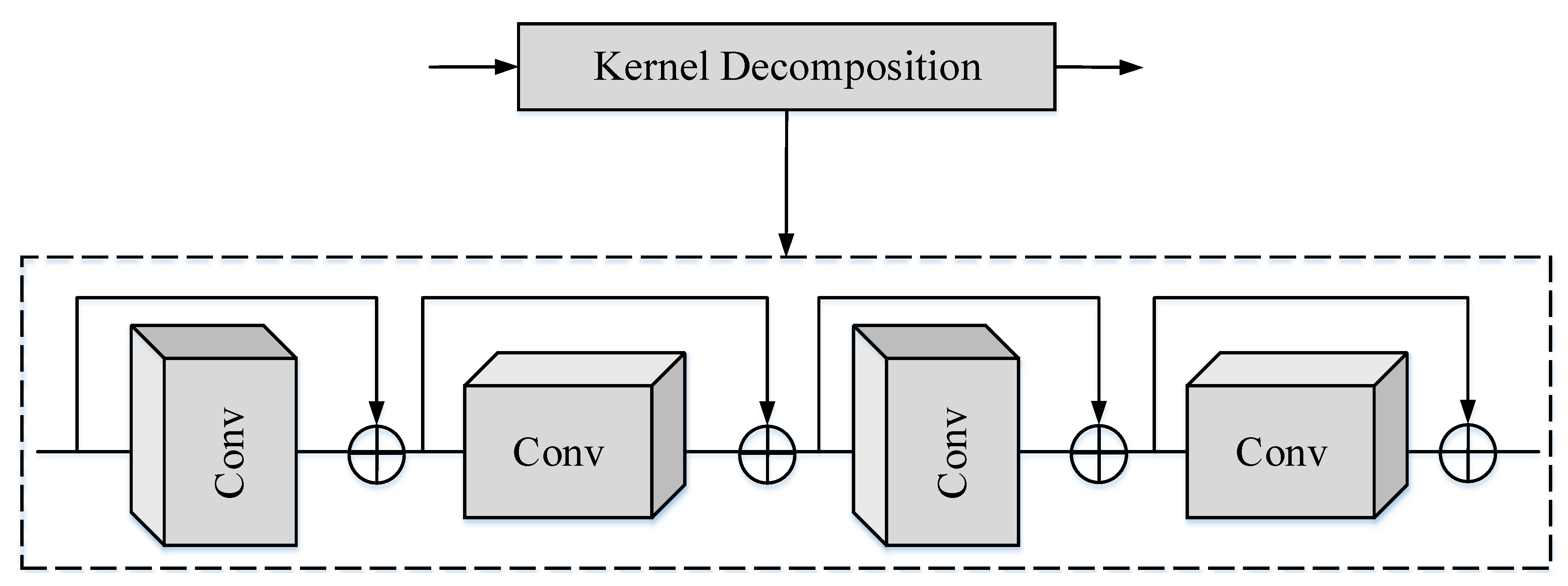
3.2.4. Kernel Decomposition
In the previous research, we found that the ResNet model introduced skip connection, which can reduce the training difficulty of the deeper deep learning model [67]. Later, in the Bi-Real-Net model, Liu et al. [71] enlarged the number of skip connections, and the performance of the model was improved. Inspired by this, in this study, we also adopted the method of adding skip connections to improve the performance of the model. A common method is to decompose the original convolution filter into pointwise convolution and depthwise convolution [72]. However, the feature representation ability of pointwise convolution in this method is limited after binarization, and there are only or states [73]. Therefore, we decompose the convolution kernel into and convolution filters to increase the number of skip connections, as shown in Figure 4. We decomposed a large convolution kernel operation into a horizontal convolution and a vertical convolution kernel in series. To enhance the performance of the model, skip connections were also introduced. In the actual algorithm design, the convolution kernel that cannot be decomposed is approximately decomposed. In the implementation of the algorithm, separable convolution filters are used.
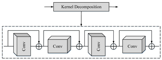
Figure 4.
Principle of kernel decomposition.
3.2.5. Residual Connection Operation
To address the problems of model degradation and slow convergence speed, the residual connection operation was adopted in this study [74]. As shown in Figure 2, the concatenate operation is regarded as increasing the depth of the model to a certain extent and enhancing the ability of the model to extract more abstract features, speed up training, and suppress the network degradation. The residual connection operation we utilize is an optimization of the above operation, providing better performance. Since Han et al. [74] demonstrated that a large number of rectified linear units (ReLU) would degrade the performance of the model, unnecessary ReLUs were removed from the residual connection operation. To ensure non-linearity, we adopt the sigmoid kernel function of the Lie Group, which is more robust and universal. The mathematical meaning of residual unit is as follows:
where represents the input of the residual unit, represents the output of the residual unit, and and represent residual operation and concatenate, respectively.
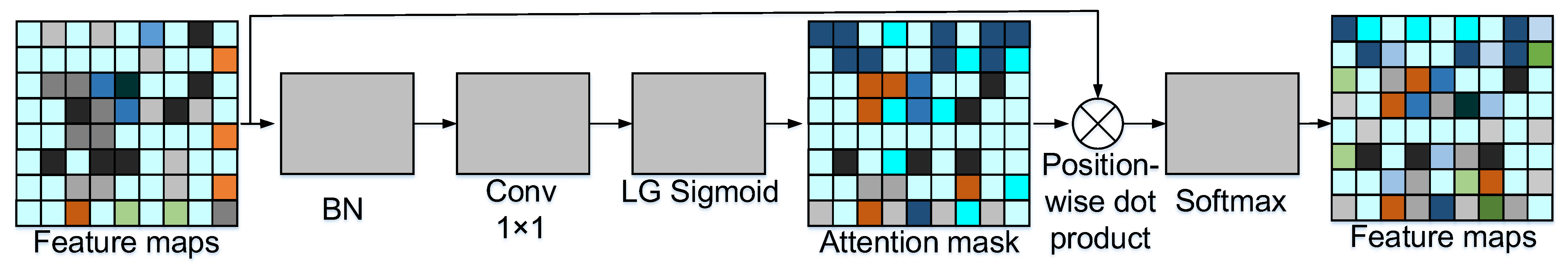
3.2.6. Spatial Attention Mechanism
In the above study, the residual connection operation is used to connect the features from different layers, which may contain some redundant features. To remove redundant features and enhance the ability of the model to extract key features [75], at the same time, to preserve more discriminative features and highlight the local features matching the scene category, in the last residual block of each flow, we add spatial attention mechanisms.
Suppose represents the feature maps output from maxpooling, represents the feature vector of a certain pixel in , and the mathematical meaning of attention weight is as follows:
where represents Lie Group Sigmoid kernel function, represents operation, represents the trainable weight parameter matrix, and b represents the bias matrix. Here, to improve the calculation speed, we utilize depthwise separable convolution.
After classical mean pooling, the mathematical meaning of the gray value of the corresponding pixel is as follows:
where represents the gray value of pixel from one of these convolutional features, and represents the window size of the pooling operation.
After attention pooling, the mathematical meaning of is as follows:
After the above operation, the important local features can be weighted and the features can be down-sampled. Figure 5 illustrates the working principle of attention weight in our proposed model:
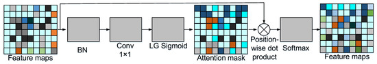
Figure 5.
Principle of spatial attention mechanism.
3.2.7. Bilinear Pooling
To enhance the representation of subtle features, we choose bilinear pooling instead of average pooling. Suppose the output of the model is , where and represent the number and channels of features, respectively. The mathematical meaning of the bilinear operation is as follows:
where represents the result of matrix multiplication for O and T. Following [76], normalization and the signed square root are applied to the bilinear pooling result . Since its gradients are available, it can be integrated into an end-to-end model.
3.3. Feature-Level Fusion Branch
Previous studies have shown that different features have their meanings and contain different attribute information [12]. Discriminant correlation analysis (DCA) is an optimization method and improvement of canonical correlation analysis [77], which can effectively reduce redundant features and maximize the pairwise correlation of different feature sets, thus obtaining compact but discriminative features. Therefore, DCA was used for feature fusion in this study.
3.3.1. Feature Fusion
Assume a heterogeneous feature set , which contains n columns and C categories, and represents the ith category. represents the jth data sample of the ith category, which can be a vector data sample or a matrix data sample. According to previous studies [20,48], firstly, we utilize the Lie Group intrinsic mean to calculate the divergence between each category:
where represents the intrinsic mean within the Lie Group of the ith category, and represents the intrinsic mean within the Lie Group of whole categories.
Then, by calculating the eigenvectors of , the dimensions of can be reduced and projected into the reduced space:
where represents a transformation using . In low-dimensional space, different categories can be distinguished. Similarly, given another heterogeneous feature set , its projection is obtained by the above steps.
The next step is to make one set of features have nonzero correlation only with the corresponding features in another set. The transformation of and is as follows:
where and represent the transformation obtained by .
Finally, the transformation is carried out in the following way, and the final feature representation is obtained:
Through the above operations, any heterogeneous features can be integrated. In addition, compared with the original heterogeneous features, the dimensionalities of the fused features are greatly reduced.
3.3.2. Loss Function
Due to the high similarity of key features in different HRRSI, the deep learning model may experience overfitting, resulting in the decline in classification accuracy. Possible solutions include the cross-entropy loss functions, thus helping improve the classification accuracy for high similarity scene categories and enhancing the generalization of the model.
According to the previous research, we found that the traditional cross-entropy loss function mainly considers the model to learn from the direction of the largest difference, and does not consider the loss of the wrong category. In practice, the remote sensing dataset contains a large number of similar scene categories. For example, the NWPU-RESISC45 dataset contains 45 categories and 31,500 images, among which only a few data samples can be used for training, and the data samples are uneven. This can easily lead to overfitting and inaccurate prediction of the model, and it is difficult to distinguish similar scene categories. Therefore, the traditional cross-entropy loss function is not enough to address the features of all data samples.
For further analysis, possible solutions include the use of a regularization strategy, that is, label smoothing; the use of hyperparameter to achieve a better trade-off between positive samples and negative samples; and the use of soft-one hot to add noise and constrain the output loss function. The cross-entropy loss relationship between the corrected real label and the corresponding probability is as follows:
where C represents the total number of categories, c represents the index of a specific category, and follows the uniform distribution of C categories. A new loss function can be obtained:
where:
where represents the actual category, and represents the corresponding probability. indicates the correctly classified category, and indicates other categories. The specific expression is as follows:
This function can satisfy the evaluation of the loss of the correct category and reduce the difference between the wrong category. In particular, it can effectively improve the difference between different scenes in remote sensing datasets and enhance the generalization of the model.
4. Experimental Results
In this section, we conduct a comprehensive experiment and analysis to evaluate the feasibility and robustness of our proposed method. Firstly, three challenging datasets used in the experiment are outlined. Secondly, the relevant settings of the experiment are described. Finally, we compared and analyzed our method with some of the state-of-the-art methods and performed ablation experiments on the modules in the model.
4.1. Experimental Datasets
In this section, we chose UC Merced [78], AID [79], and NWPU-RESISC45 [25], three public and challenging datasets. The UC Merced dataset [78] contains 21 land-use scenes with a total of 2100 images. The AID dataset [79] contains 30 scene types, each with 200 to 400 images. The NWPU-RESISC45 dataset [25], published by Northwestern Polytechnical University, contains 45 scene classes with a total of 31,500 images. The above dataset has the following characteristics: (1) They are the most influential of the remote sensing datasets, which have been widely used in the classification and retrieval of remote sensing image scenes; (2) the diversity of images, taking into account the different times, seasons, and imaging conditions of the scene; (3) the image contains variations in spatial resolution, viewpoint, occlusion, and background, which increase the challenge of classification; (4) the scale of the remote sensing scene dataset is significantly expanded, with large intraclass differences and high interclass similarity. To prevent overfitting, data augmentations were used to supplement the number of datasets during the experiment, including horizontal and vertical flipping and rotation at different angles.
4.2. Experiment Setup
The model is implemented based on the deep learning platform of Tensorflow [80]. The model was optimized by stochastic gradient descent (SGD) algorithm. The experimental environment settings are shown in Table 2. After the initial setting is completed, the initial learning rate is reduced by 105 times while observing the validation loss decreasing slowly.
Table 2.
Experimental environment parameters.
To fairly compare with other experimental models, we stipulate that the ratio of the training set and test set should be the same as that of most previous models [25]. The evaluation indicators include the overall accuracy (OA), the Kappa coefficient (KC), and the confusion matrix. To obtain reliable experimental results, we randomly divided three datasets according to the ratio of training and test sets, repeated the experiment 10 times, and calculated the standard deviation and average value to obtain the final experimental results.
4.3. Experimental Results
Previous studies have shown [25,79] that the model based on CNN far surpassed the method based on shallower features. Therefore, in this experiment, we did not choose to compare with the traditional method based on handcrafted features.
The experimental results are shown in Table 3, as follows:
Table 3.
In the experimental results under three different datasets of UC Merced (UCM), AID, and NWPU-RESISC45 (NWPU), we utilized 24 models to compare the overall accuracy (OA%) and Kappa coefficient (KC) with our proposed model.
The experimental results on the UCM dataset are listed below:
- When the training ratio is 50%, the accuracy of our proposed model achieves 98.67%, surpassing all the previous models. The experimental results indicate that the classification accuracy can be improved effectively by adding shallower features (low-level and middle-level features), parallel dilated convolution, Lie Group kernel function, kernel decomposition, and skip connection. Shallower features and multidilation pooling modules are used in LGRIN [12], but the classification accuracy of our model is 0.06% higher than that of LGRIN [12]. Our model is 0.19% higher than CSCD [8], 0.1% higher than SEMDPMNet [81], and 5.91% higher than Xception [82]. When the training ratio is 80%, our proposed model is 3.45% high than MobileNet V2 [81] and 0.02% higher than SCC-CNN [37].
- In addition, we also analyzed the Kappa coefficient corresponding to the above models. When the training ratio is 50%, the Kappa coefficient of our model is 98.31%, which is 4.04% higher than that of APDC-NET [16] and 2.74% higher than that of LCPB [83]. When the training ratio is 80%, the Kappa coefficient of our model is 99.76%, which is 0.01% higher than that of LCNN-GWHA [38] and 0.26% higher than that of LCNN-CMGF [40]. The above experimental results verify the superiority of our model.
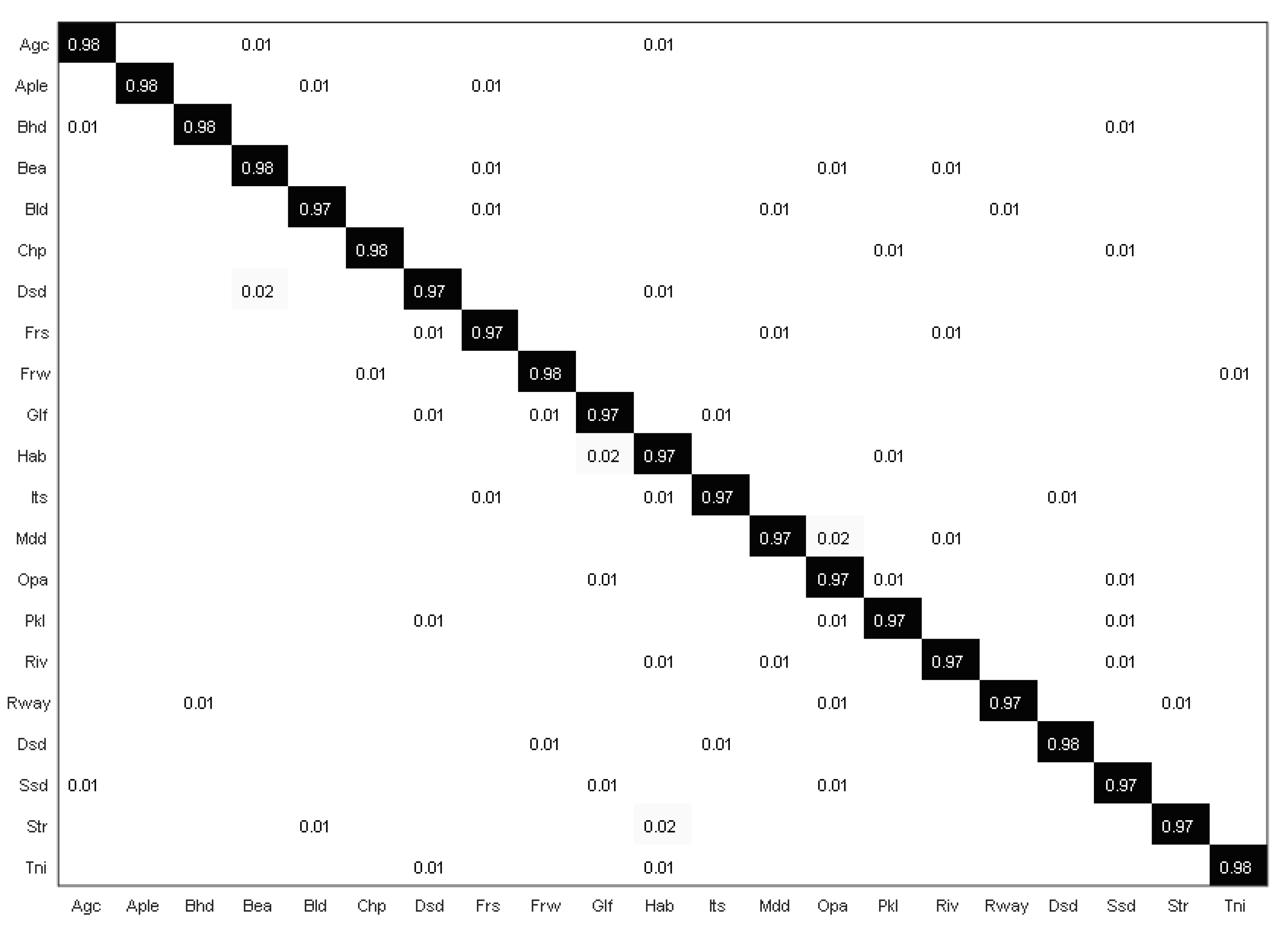
- As shown in Figure 6, our proposed model fully recognized most of the scene categories, and the recognition rate of the medium residential and dense residential scene is lower than that of other scenes. Therefore, we believe that there is a large confusion between them, mainly because their distribution is quite similar, and the difference between the extracted shallower features and the high-level features is small.
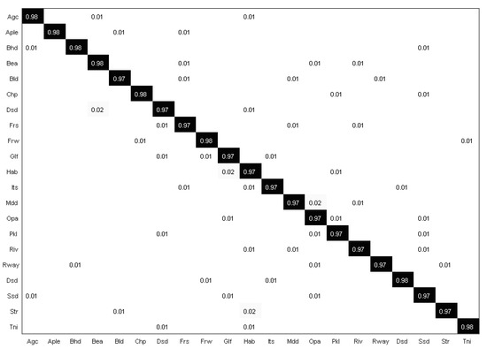 Figure 6. Confusion matrix of our proposed method with the UC Merced dataset.
The experimental results on the AID dataset are presented below:
- The AID dataset is different from UCM dataset. The AID dataset is multi-sourced: It is collected from different regions of the world with different spatial resolutions and times. In addition, these images are captured by different sensors, which makes scene classification more difficult. When the training ratio is 20%, the accuracy of our proposed model achieves 94.79%, 7.11% higher than LCPB [83], 3.83% higher than LCPP [83], and 0.16% higher than DF-CNN [41]. When the training ratio is 50%, the accuracy of our proposed model achieves 97.72%, 0.41% higher than SCC-CNN [37], 0.08% higher than LCNN-GWHA [38], and 3.03% higher than ResNet50 [85].
- When the training ratio is 20%, the Kappa coefficient our proposed achieves 94.57%, which is 9.2% and 0.11% higher than VGG-VD-16 [79] and DF-CNN [41], respectively, and 9.34% higher than CaffeNet [79]. When the training ratio is 50%, the Kappa coefficient our proposed achieves 97.61%, which is 0.16% higher than LCNN-CMGF [40], 0.06% higher than LCNN-GWHA [38], and 1.58% higher than SCC-CNN [37].
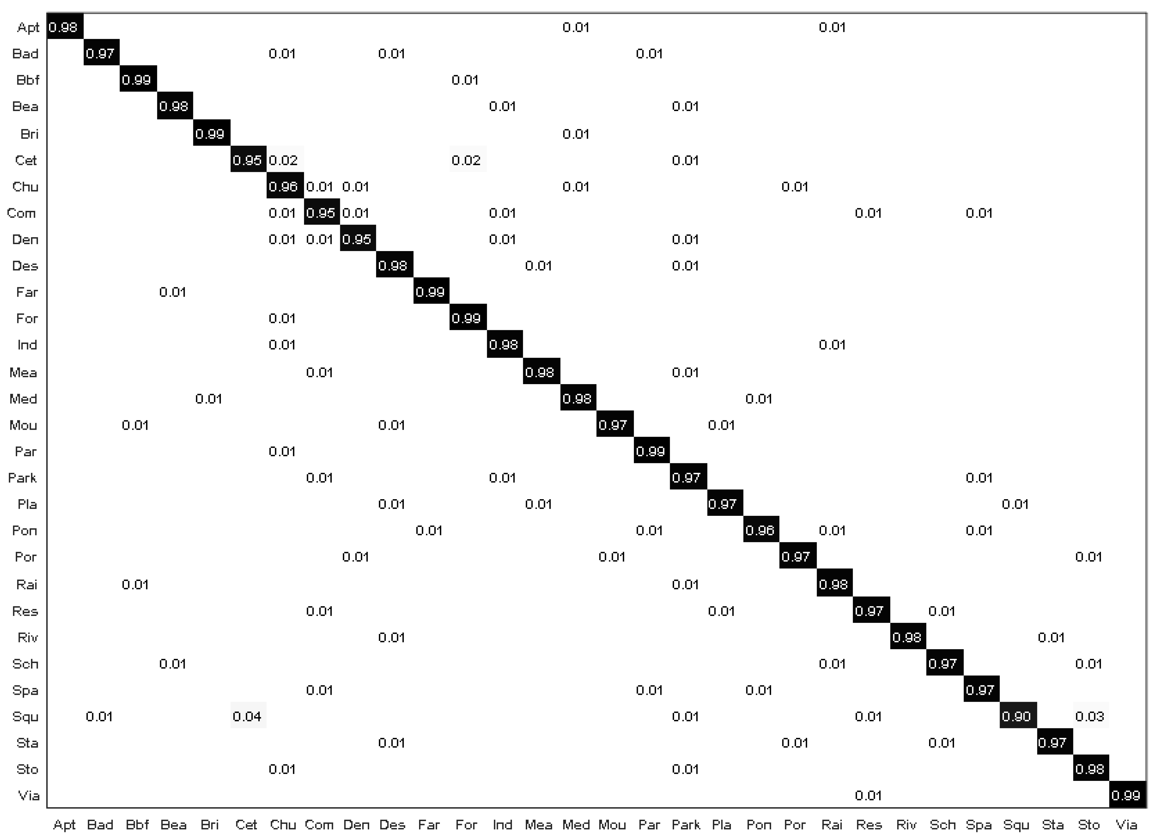
- As for the confusion matrix shown in Figure 7, our model can achieve 96% in most scenes, and 100% in some scenes, such as in parks and forests. However, the classification accuracy of some scenes is low. After further analysis, we found that their structure and composition are highly similar, such as the shallower features of ponds and buildings, so the classification accuracy is low.
 Figure 7. Confusion matrix of our proposed method with the AID dataset.
The experimental results on the NWPU dataset are listed below:
- The NWPU dataset is large in terms of the total number of categories of images and scenes. In addition, the dataset has large intraclass differences and high interclass similarity, and it contains variations in spatial resolution, viewpoint, illumination, occlusion, and background, which represents a more challenging scene classification task than the UCM and AID datasets. When the training ratio is 10%, the accuracy of our proposed model achieves 92.62%, which is 0.09% higher than that of LCNN-CMGF [38], 0.71% higher than that of LGRIN [12], and 0.38% higher than that of LCNN-GWHA [38]. When the training ratio is 20%, the accuracy of our proposed model achieves 94.49%, which is 0.9% higher than that of CSCD [8], 0.06% higher than that of LGRIN [12], and 0.38% higher than that of SE-MDPMNET [81].
- When the training ratio is 10%, the Kappa coefficient of our proposed model achieves 92.25%, which is 0.21% and 0.08% higher than LCNN-GWHA [38] and LCNN-CMGF [40], respectively. When the training rate is 20%, the accuracy of our proposed model achieves 94.31%, which is 0.08% higher than DF-CNN [41], 0.27% higher than LCNN-CMGF [40], and 1.03% higher than LGRIN [12].
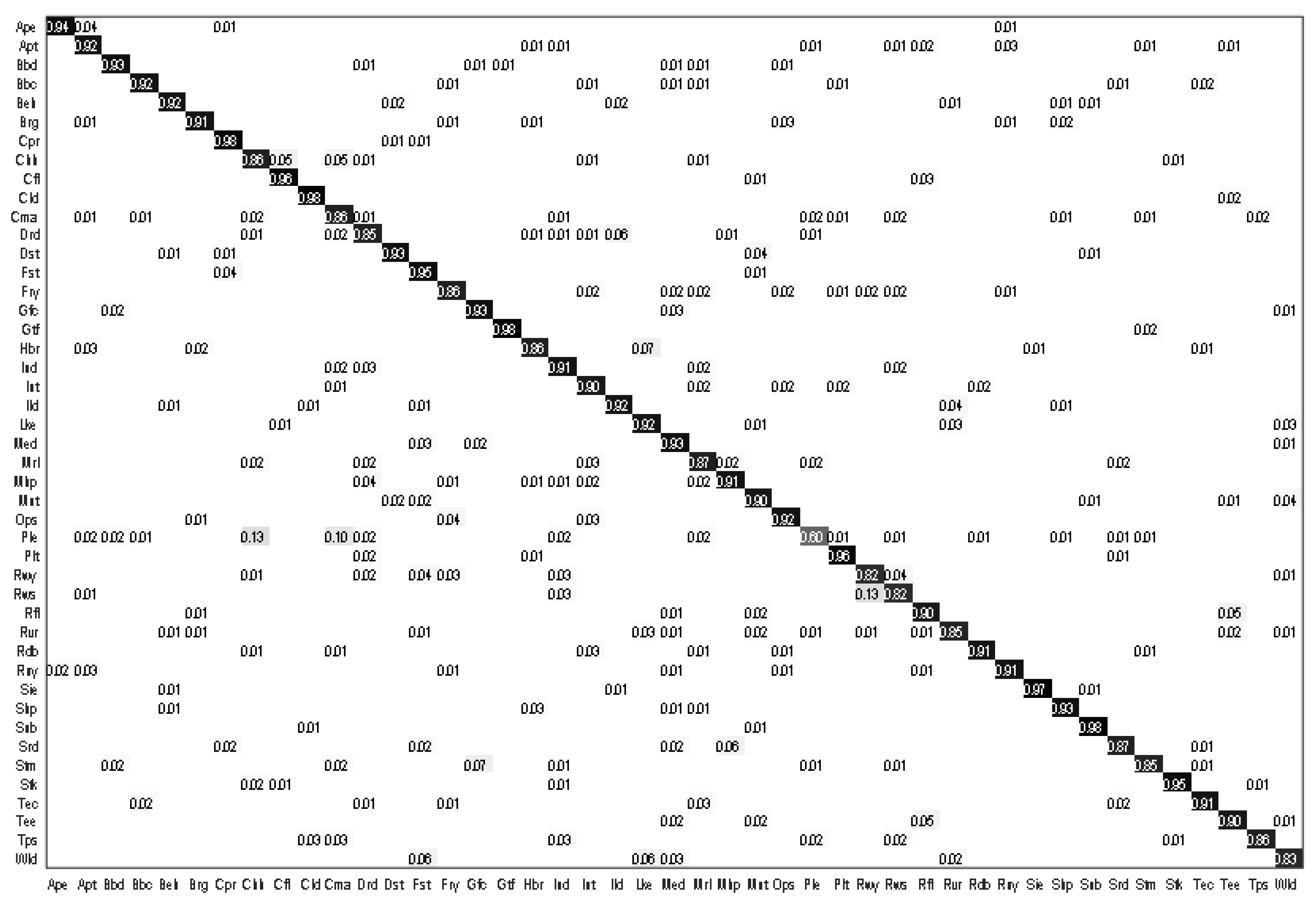
- Confusion matrix as shown in Figure 8: Similar to the AID dataset, the classification accuracy of our proposed model can achieve 92% in most scenarios. Due to the large scale of NWPU datasets, large intraclass differences, and high interclass similarity, none of the categories are completely correctly classified. Because churches and palaces have similar physical structures and other characteristics, these two kinds of scenes are easy to be confused.
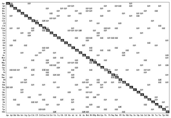 Figure 8. Confusion matrix of our proposed method with the NWPU-RESISC45 dataset.
5. Discussion
The above results can be explained from the following aspects:
- The existing CNNs model tends to retain the high-level features while ignoring the shallower features in the image, resulting in the classification accuracy of the scene being relatively low. However, the model of our proposed efficiently integrates different features of multiple levels, especially the shallower features, providing more features required by the model and effectively improves the classification accuracy of the scene;
- Our proposed model adopts a spatial attention mechanism, kernel decomposition, and the method of increasing the number of skip connections. It can effectively extract more important weight feature information in the image and preserve the feature information of different levels, making the extracted feature more discriminative to the scene;
- Generally, deeper and wider models can extract more global features, but it is easy to increase the complexity and number of parameters of the model, and it is also easy to extract features through pure linear stacked convolution modules, thus affecting the classification accuracy. In our model, skip connections, parallel dilated convolution, and expanded kernel size was used to expand the receptive field and extract more global features, which effectively reduced the number of parameters and complexity of the model and improved the classification accuracy;
- The pyramid residual connection is adopted in our proposed model, which can not only reduce the complexity of the model but also reuse parameters and features, reduce the parameters of the model, enhance the feature learning ability of the model, and establish connections with shallower features. In other words, the pyramid residual connection further reduces the computational complexity and the number of model parameters and ensures the ability of the model to extract deeper features.
5.1. Evaluation of Size of Models
In this experiment, we select 10 classical models to compare the size of the model, namely, CaffeNet [79], GoogLeNet [79], MobileNet V2 [81], SE-MDPMNet [81], ResNet50 [85], VGG-VD-16 [79], Inception V3 [85], LCNN-GWHA [38], SCC-CNN [8] and LGRIN [12], where GMACs represent the complexity of computation. From Table 4, we found that compared with SE-MDPMNet [81], our model has advantages in terms of parameter number and GMACs. In addition, compared with lightweight models, GoogLeNet [79] and MobileNet [81], our model achieves a better trade-off between OA, model parameters, and GMACs. Since parallel dilated convolution is adopted in our model, compared with LCNN-GWHA [38], our model reduces the number of parameters and further improves the computational performance of the model. Our model has much fewer parameters, but the classification accuracy is still better than other CNN models. In addition, the time complexity of the model is in the best case and in the worst case.
Table 4.
Taking AID (50%) as an example, the size of the model is evaluated.
5.2. Comparison of Prediction Time
As shown in Table 5, the prediction time of a single HRRSI from each of the three datasets is compared. The prediction time of our model is significantly reduced compared with other models. The experimental results in Table 5 show that the reduction in the parameters in the model is beneficial to improving the prediction time of the model. There is little difference in the number of parameters between our proposed model and LCNN-GWHA [38], but our prediction speed is 0.015S (on average) faster than LCNN-GWHA [38], which shows that the kernel size and receptive field are increased in parallel dilated convolution, and the computational performance of the model is not reduced.
Table 5.
Prediction times (S) of different models with three datesets.
5.3. Ablation Experiment
Taking the AID (50%) dataset as an example, we conducted a series of experiments to analyze the effect of each module in the model. To ensure a fair comparison, all evaluated are set with the same parameters.
5.3.1. Effects of LGML in the Model
To clarify the effect of LGML in the model, two different structures are designed based on dense connected convolutional neural network (DCCNN) and LGML. DCCNN is a model used to retain shallower features [88]. The experimental results are shown in Table 6: It has been shown that the model based on LGML has good performance. The relative improvements of each metric approximates 4% to 5%. The characterization method of the Lie Group feature matrix in LGML adopts a real symmetric matrix. Compared with the DCCNN model, it has fewer parameters, good computational performance, and an anti-noise ability. In addition, it can better express features and their correlation between features, and improve the comprehensibility of the model from the perspective of LGML.
Table 6.
Influence of LGML.
5.3.2. Effect of Spatial Attention Mechanism
To confirm the effect of spatial attention mechanism on the model, we compared our classification results with the model without spatial attention mechanism, and the results are shown in Table 7. Our proposed model achieves the highest classification accuracy, and the spatial attention mechanism improves the classification accuracy of the model by 3.36%. These experimental results indicate that the spatial attention mechanism in the model is beneficial to scene classification.
Table 7.
Influence of spatial attention mechanism.
5.3.3. Influence of Different Distance Space Calculation Methods on Model Scene Classification
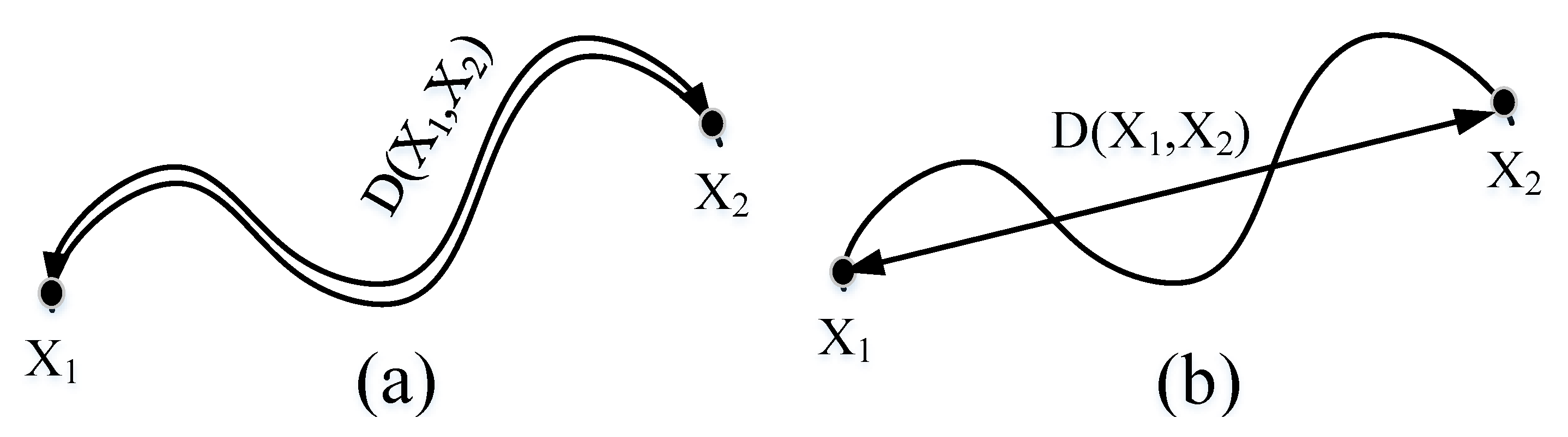
Since most of the existing CNN models utilize Euclidean space distance for calculation, in practical application scenarios, Euclidean space distance is mainly applicable to vector space data samples, and there are limitations for non-Euclidean space samples. As shown in Figure 9, Figure 9a is the distance calculated by using Lie Group manifold distance, and Figure 9b is the distance directly calculated by using Euclidean space distance. Obviously, the manifold space distance can better reflect the real distance between data samples. As shown in Table 8, the experimental results obtained by calculating Euclidean space distance and manifold space distance are adopted, respectively. The experimental results show that the manifold space distance can achieve higher classification accuracy.
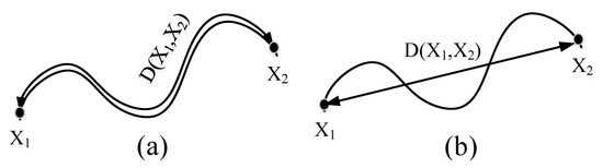
Figure 9.
Difference of Manifold distance and Euclidean distance: (a) represents the distance between the samples and on the manifold space of the Lie Group, and the distance is on the manifold space; (b) is the distance obtained by directly using Euclidean distance to calculate samples and .
Table 8.
Influence of different distance space calculation methods.
5.3.4. Contribution of Pyramid Residual Connection and Bilinear Pooling to the Model
To verify the effects of pyramid residual connection and bilinear pooling, we compare our classification results (i.e., using pyramid residual connection and bilinear pooling, PRC + BIP) with the following three situations, that is, using the residual connection and global average pooling (RC + GAP), residual connection and bilinear pooling (RC + BIP), pyramid residual connection and global average pooling (PRC + GAP). All experimental results are listed in Table 9 and can also be found follows:
Table 9.
Influence of pyramid residual connection and bilinear pooling to the model.
- In all experiments, the proposed model achieves the highest classification accuracy, while RC + GAP achieves the lowest classification accuracy;
- Compared with PRU + GAP, our classification accuracy is improved by 4.31%, indicating that the model based on bilinear pooling has better classification performance. We can consider that this method can provide many subtle and discriminative features for the model;
- The experimental results indicate that both the pyramid residual connection and bilinear pooling are beneficial to scene classification. In addition, as shown in Figure 1, the pyramid connecting is also beneficial to the convergence of the model and improves the fitting effect of the model.
5.3.5. Influence of Cross-Entropy Loss Function on Model Scene Classification
To verify that the traditional cross-entropy loss function (CEL) and cross-entropy loss function based on label smoothing (CELLS) influence scene classification, we compare our classification results with the model using the traditional cross-entropy loss function. The experimental results are shown in Table 10. The classification accuracy of CELLS is 2.34% higher than that of the CEL model, which shows that CELLS is more suitable for scene classification. Label smoothing corrects the loss function and improves the generalization ability of the model.
Table 10.
Influence of cross-entropy loss function on model scene classification.
6. Conclusions
Intraclass diversity and interclass similarities are existing in HRRSIs, which have complex spatial distributions and geometric structures. The traditional CNN model based on linear superposition cannot extract key and discriminative features. Therefore, this study proposes a novel Lie Group deep learning model to address the above problems. Firstly, by combining LGML and deep learning, our proposed model jointly learns shallower features (low-level and middle-level features) and high-level features (semantic features). In this model, the parallel dilated convolution, Lie Group kernel function, kernel decomposition, and pyramid residual connection are adopted to expand the receptive field, reduce the number of parameters and calculation, prevent model degradation and overfitting, and effectively extract the key and discriminative features at different levels. Secondly, the spatial attention mechanism in the model can effectively suppress irrelevant feature information and enhance local semantic features. Finally, the feature-level fusion method is adopted to avoid feature redundancy and reduce the dimension of feature, enhance the capability of feature representation and maintain good computing performance. In addition, to reduce the influence of high similarity categories on scene classification, the model adopts the cross-entropy loss function based on label smoothing. The proposed model is performed on three public and challenging large-scale datasets, and the experimental results verify that our method has better performance than other methods.
Author Contributions
Conceptualization, C.X., G.Z. and J.S.; methodology, C.X.; software, J.S.; validation, C.X. and G.Z.; formal analysis, J.S.; investigation, C.X.; resources, C.X. and G.Z.; data curation, J.S.; writing—original draft preparation, C.X.; writing—review and editing, C.X.; visualization, J.S.; supervision, J.S.; project administration, J.S.; funding acquisition, C.X. All authors have read and agreed to the published version of the manuscript.
Funding
This research was funded by the Science and Technology Foundation of Education Department of Jiangxi Province, China. Grant No. GJJ203204.
Institutional Review Board Statement
Not applicable.
Informed Consent Statement
Not applicable.
Data Availability Statement
Data associated with this research are available online. The UC Merced dataset is available for download at http://weegee.vision.ucmerced.edu/datasets/landuse.html (accessed on 12 November 2021). RSCCN dataset is available for download at https://sites.google.com/site/qinzoucn/documents (accessed on 10 October 2020). NWPU dataset is available for download at http://www.escience.cn/people/JunweiHan/NWPURE-SISC45.html (accessed on 16 October 2020). AID dataset is available for download at https://captain-whu.github.io/AID/ (accessed on 15 December 2021).
Acknowledgments
The authors would like to thank two anonymous reviewers for carefully reviewing this study and giving valuable comments to improve this study.
Conflicts of Interest
The authors declare no conflict of interest.
Abbreviations
| AID | Aerial Image Dataset |
| BoVW | Bag-of-Visual-Words |
| CBAM | Convolutional Block Attention Module |
| CH | Color Histogram |
| CNN | Convolutinal Neural Network |
| DCA | Discriminant Correlation Analysis |
| DCCNN | Dense Connected Convolutional Neural Network |
| DepConv | Depth separable Convolutions |
| F1 | F1 score |
| GAN | Generative Adversarial Network |
| HRRSI | High-resolution Remote Sensing Images |
| KC | Kappa Coefficient |
| LBP | Local Binary Pattern |
| LDA | Latent Dirichlet Allocation |
| LGDL | Lie Group Deep Learning |
| LGML | Lie Group Machine Learning |
| LGRIN | Lie Group Regional Influence Network |
| OA | Overall Accuracy |
| PGA | Principal Geodesic Analysis |
| PLSA | Probabilistic Latent Semantic Analysis |
| PTM | Probabilistic Topic Models |
| ReLU | Rectified Linear Units |
| SGD | Stochastic Gradient Descent |
| SIFT | Scale-invariant Feature Transform |
References
- Cheng, G.; Xie, X.; Han, J.; Guo, L.; Xia, G.S. Remote sensing image scene classification meets deep learning: Challenges, methods, benchmarks, and opportunities. IEEE J. Sel. Top. Appl. Earth Obs. Remote Sens. 2020, 13, 3735–3756. [Google Scholar] [CrossRef]
- Li, D.; Wang, M.; Dong, Z.; Shen, X.; Shi, L. Earth observation brain (EOB): An intelligent earth observation system. Geo-Spat. Inf. Sci. 2017, 20, 134–140. [Google Scholar] [CrossRef] [Green Version]
- Chen, W.; Li, X.; He, H.; Wang, L. Assessing different feature sets’ effects on land cover classification in complex surface-mined landscapes by ZiYuan-3 satellite imagery. Remote Sens. 2018, 10, 23. [Google Scholar] [CrossRef] [Green Version]
- Li, K.; Wan, G.; Cheng, G.; Meng, L.; Han, J. Object detection in optical remote sensing images: A survey and a new benchmark. ISPRS J. Photogramm. Remote Sens. 2020, 159, 296–307. [Google Scholar] [CrossRef]
- Cheng, G.; Han, J.; Zhou, P.; Xu, D. Learning rotation-invariant and fisher discriminative convolutional neural networks for object detection. IEEE Trans. Image Process. 2019, 28, 265–278. [Google Scholar] [CrossRef]
- Lv, Z.Y.; Shi, W.; Zhang, X.; Benediktsson, J.A. Landslide inventory mapping from bitemporal high-resolution remote sensing images using change detection and multiscale segmentation. IEEE J. Sel. Top. Appl. Earth Observ. Remote Sens. 2018, 11, 1520–1532. [Google Scholar] [CrossRef]
- Longbotham, N.; Chaapel, C.; Bleiler, L.; Padwick, C.; Emery, W.J.; Pacifici, F. Very high resolution multiangle urban classification analysis. IEEE Trans. Geosci. Remote Sens. 2012, 50, 1155–1170. [Google Scholar] [CrossRef]
- Wang, X.; Yuan, L.; Xu, H.; Wen, X. CSDS: End-to-End Aerial Scenes Classification With Depthwise Separable Convolution and an Attention Mechanism. IEEE J. Sel. Top. Appl. Earth Obs. Remote Sens. 2021, 14, 10484–10499. [Google Scholar] [CrossRef]
- Zhu, Q.; Zhong, Y.; Zhang, L.; Li, D. Adaptive deep sparse semantic modeling framework for high spatial resolution image scene classification. IEEE Trans. Geosci. Remote Sens. 2018, 56, 6180–6195. [Google Scholar] [CrossRef]
- Cheng, G.; Yang, C.; Yao, X.; Guo, L.; Han, J. When deep learning meets metric learning: Remote sensing image scene classification via learning discriminative CNNs. IEEE Trans. Geosci. Remote Sens. 2018, 56, 2811–2821. [Google Scholar] [CrossRef]
- Anwer, R.M.; Khan, F.S.; van de Weijer, J.; Molinier, M.; Laaksonen, J. Binary patterns encoded convolutional neural networks for texture recognition and remote sensing scene classification. ISPRS J. Photogramm. Remote Sens. 2018, 138, 74–85. [Google Scholar] [CrossRef] [Green Version]
- Xu, C.; Zhu, G.; Shu, J. A Lightweight and Robust Lie Group-Convolutional Neural Networks Joint Representation for Remote Sensing Scene Classification. IEEE Trans. Geosci. Remote Sens. 2022, 60, 1–15. [Google Scholar] [CrossRef]
- He, Q.; Sun, X.; Yan, Z.; Fu, K. DABNet: Deformable contextual and boundary-weighted network for cloud detection in remote sensing images. IEEE Trans. Geosci. Remote Sens. 2022, 60, 1–16. [Google Scholar] [CrossRef]
- Chaib, S.; Liu, H.; Gu, Y.; Yao, H. Deep feature fusion for VHR remote sensing scene classification. IEEE Trans. Geosci. Remote Sens. 2017, 55, 4775–4784. [Google Scholar] [CrossRef]
- Li, E.; Xia, J.; Du, P.; Lin, C.; Samat, A. Integrating multilayer features of convolutional neural networks for remote sensing scene classification. IEEE Trans. Geosci. Remote Sens. 2017, 55, 5653–5665. [Google Scholar] [CrossRef]
- Bi, Q.; Qin, K.; Zhang, H.; Xie, J.; Li, Z.; Xu, K. APDC-Net: Attention pooling-based convolutional network for aerial scene classification. IEEE Geosci. Remote Sens. Lett. 2020, 17, 1603–1607. [Google Scholar] [CrossRef]
- Hu, F.; Xia, G.S.; Hu, J.; Zhang, L. Transferring deep convolutional neural networks for the scene classification of high-resolution remote sensing imagery. Remote Sens. 2015, 7, 14680–14707. [Google Scholar] [CrossRef] [Green Version]
- Luus, F.P.; Salmon, B.P.; Van den Bergh, F.; Maharaj, B.T.J. Multiview deep learning for land-use classification. IEEE Geosci. Remote Sens. Lett. 2015, 12, 2448–2452. [Google Scholar] [CrossRef] [Green Version]
- Yang, N.; Tang, H.; Sun, H.; Yang, X. DropBand: A simple and effective method for promoting the scene classification accuracy of convolutional neural networks for VHR remote sensing imagery. IEEE Geosci. Remote Sens. Lett. 2018, 15, 257–261. [Google Scholar] [CrossRef]
- Xu, C.; Zhu, G.; Shu, J. Robust Joint Representation of Intrinsic Mean and Kernel Function of Lie Group for Remote Sensing Scene Classification. IEEE Geosci. Remote Sens. Lett. 2020, 118, 796–800. [Google Scholar] [CrossRef]
- Zhang, W.; Tang, P.; Zhao, L. Remote sensing image scene classification using CNN-CapsNet. Remote Sens. 2019, 11, 494. [Google Scholar] [CrossRef] [Green Version]
- Ji, J.; Zhang, T.; Jiang, L.; Zhong, W.; Xiong, H. Combining multilevel features for remote sensing image scene classification with attention model. IEEE Geosci. Remote Sens. Lett. 2020, 17, 1647–1651. [Google Scholar] [CrossRef]
- Ma, C.; Mu, X.; Lin, R.; Wang, S. Multilayer feature fusion with weight adjustment based on a convolutional neural network for remote sensing scene classification. IEEE Geosci. Remote Sens. Lett. 2020, 18, 241–245. [Google Scholar] [CrossRef]
- Wang, X.; Xu, M.; Xiong, X.; Ning, C. Remote Sensing Scene Classification Using Heterogeneous Feature Extraction and Multi-Level Fusion. IEEE Access 2020, 8, 217628–217641. [Google Scholar] [CrossRef]
- Cheng, G.; Han, J.; Lu, X. Remote sensing image scene classification: Benchmark and state of the art. Proc. IEEE 2017, 105, 1865–1883. [Google Scholar] [CrossRef] [Green Version]
- Lee, C.Y.; Gallagher, P.; Tu, Z. Generalizing pooling functions in cnns: Mixed, gated, and tree. IEEE Trans. Pattern Anal. Mach. Intell. 2018, 40, 863–875. [Google Scholar] [CrossRef]
- Ma, B.; Hu, H.; Shen, J.; Liu, Y.; Shao, L. Generalized pooling for robust object tracking. IEEE Trans. Image Process. 2016, 25, 4199–4208. [Google Scholar] [CrossRef] [Green Version]
- Lowe, D.G. Distinctive image features from scale-invariant keypoints. Int. J. Comput. Vis. 2004, 60, 91–110. [Google Scholar] [CrossRef]
- Ojala, T.; Pietikainen, M.; Maenpaa, T. Multiresolution gray-scale and rotation invariant texture classification with local binary patterns. IEEE Trans. Pattern Anal. Mach. Intell. 2002, 24, 971–987. [Google Scholar] [CrossRef]
- Swain, M.J.; Ballard, D.H. Color indexing. Int. J. Comput. Vis. 1991, 7, 11–32. [Google Scholar] [CrossRef]
- Avramović, A.; Risojević, V. Block-based semantic classification of high-resolution multispectral aerial images. Signal Image Video Process. 2016, 10, 75–84. [Google Scholar] [CrossRef]
- Zhu, Q.; Zhong, Y.; Zhao, B.; Xia, G.S.; Zhang, L. Bag-of-visual-words scene classifier with local and global features for high spatial resolution remote sensing imagery. IEEE Geosci. Remote Sens. Lett. 2016, 13, 747–751. [Google Scholar] [CrossRef]
- Blei, D.M.; Ng, A.Y.; Jordan, M.I. Latent dirichlet allocation. J. Mach. Learn. Res. 2003, 3, 993–1022. [Google Scholar]
- Hofmann, T. Unsupervised learning by probabilistic latent semantic analysis. Mach. Learn. 2001, 42, 177–196. [Google Scholar] [CrossRef]
- Zhao, B.; Zhong, Y.; Xia, G.S.; Zhang, L. Dirichlet-derived multiple topic scene classification model for high spatial resolution remote sensing imagery. IEEE Trans. Geosci. Remote Sens. 2015, 54, 2108–2123. [Google Scholar] [CrossRef]
- Zhong, Y.; Fei, F.; Liu, Y.; Zhao, B.; Jiao, H.; Zhang, L. SatCNN: Satellite image dataset classification using agile convolutional neural networks. Remote Sens. Lett. 2017, 8, 136–145. [Google Scholar] [CrossRef]
- Shi, C.; Zhang, X.; Sun, J.; Wang, L. Remote Sensing Scene Image Classification Based on Self-Compensating Convolution Neural Network. Remote Sens. 2022, 14, 545. [Google Scholar] [CrossRef]
- Shi, C.; Zhang, X.; Sun, J.; Wang, L. A Lightweight Convolutional Neural Network Based on Group-Wise Hybrid Attention for Remote Sensing Scene Classification. Remote Sens. 2022, 14, 161. [Google Scholar] [CrossRef]
- Zhang, Z.; Liu, S.; Zhang, Y.; Chen, W. RS-DARTS: A Convolutional Neural Architecture Search for Remote Sensing Image Scene Classification. Remote Sens. 2022, 14, 141. [Google Scholar] [CrossRef]
- Shi, C.; Zhang, X.; Wang, L. A Lightweight Convolutional Neural Network Based on Channel Multi-Group Fusion for Remote Sensing Scene Classification. Remote Sens. 2022, 14, 9. [Google Scholar] [CrossRef]
- Wang, D.; Lan, J. A Deformable Convolutional Neural Network with Spatial-Channel Attention for Remote Sensing Scene Classification. Remote Sens. 2021, 13, 5076. [Google Scholar] [CrossRef]
- Krizhevsky, A.; Sutskever, I.; Hinton, G.E. Imagenet classification with deep convolutional neural networks. Commun. ACM 2017, 60, 84–90. [Google Scholar] [CrossRef]
- Goodfellow, I.; Pouget-Abadie, J.; Mirza, M.; Xu, B.; Warde-Farley, D.; Ozair, S.; Bengio, Y. Generative adversarial nets. Adv. Neural Inf. Process. Syst. 2014, 27, 2672–2680. [Google Scholar]
- Hinton, G.E.; Salakhutdinov, R.R. Reducing the dimensionality of data with neural networks. Science 2006, 313, 504–507. [Google Scholar] [CrossRef] [PubMed] [Green Version]
- Zhao, L.; Tang, P.; Huo, L. Feature significance-based multibag-of-visual-words model for remote sensing image scene classification. J. Appl. Remote Sens. 2016, 10, 35004. [Google Scholar] [CrossRef]
- Zhong, Y.; Zhu, Q.; Zhang, L. Scene classification based on the multifeature fusion probabilistic topic model for high spatial resolution remote sensing imagery. IEEE Trans. Geosci. Remote Sens. 2015, 53, 6207–6222. [Google Scholar] [CrossRef]
- Gilmore, R. Lie Groups, Lie Algebras, and Some of Their Applications; Courier Corporation: New York, NY, USA, 2012. [Google Scholar]
- Xu, C.; Zhu, G.; Shu, J. A Lightweight Intrinsic Mean for Remote Sensing Classification With Lie Group Kernel Function. IEEE Geosci. Remote Sens. Lett. 2020, 18, 1741–1745. [Google Scholar] [CrossRef]
- Lin, D.; Grimson, E.; Fisher, J. Learning visual flows: A Lie algebraic approach. In Proceedings of the 2009 IEEE Conference on Computer Vision and Pattern Recognition, Miami, FL, USA, 20–25 June 2009; pp. 747–754. [Google Scholar] [CrossRef] [Green Version]
- Tuzel, O.; Porikli, F.; Meer, P. Region covariance: A fast descriptor for detection and classification. In Proceedings of the European Conference on Computer, 9th European Conference on Computer Vision, Graz, Austria, 7–13 May 2006; Springer: Berlin/Heidelberg, Germany, 2006; pp. 589–600. [Google Scholar] [CrossRef]
- Tuzel, O.; Porikli, F.; Meer, P. Human detection via classification on riemannian manifolds. In Proceedings of the 2007 IEEE Conference on Computer Vision and Pattern Recognition, Minneapolis, MN, USA, 17–22 June 2007; pp. 1–8. [Google Scholar] [CrossRef] [Green Version]
- Tran, T.N.; Yoshinaga, M. Combinatorics of certain abelian Lie group arrangements and chromatic quasi-polynomials. J. Comb. Theory 2019, 165, 258–272. [Google Scholar] [CrossRef] [Green Version]
- Fletcher, P.T.; Lu, C.; Joshi, S. Statistics of shape via principal geodesic analysis on Lie groups. In Proceedings of the 2003 IEEE Computer Society Conference on Computer Vision and Pattern Recognition, Madison, WI, USA, 18–20 June 2003; Volume 1, p. 1. [Google Scholar] [CrossRef] [Green Version]
- Yarlagadda, P.; Ozcanli, O.; Mundy, J. Lie group distance based generic 3-d vehicle classification. In Proceedings of the 19th International Conference on Pattern Recognition, Tampa, FL, USA, 8–11 December 2008; pp. 1–4. [Google Scholar] [CrossRef]
- Itti, L.; Koch, C.; Niebur, E. A model of saliency-based visual attention for rapid scene analysis. IEEE Trans. Pattern Anal. Mach. Intell. 1998, 20, 1254–1259. [Google Scholar] [CrossRef] [Green Version]
- Woo, S.; Park, J.; Lee, J.Y.; Kweon, I.S. Cbam: Convolutional block attention module. In Proceedings of the European Conference on Computer Vision (ECCV), Munich, Germany, 8–14 September 2018; pp. 3–19. [Google Scholar]
- Hu, J.; Xia, G.S.; Hu, F.; Sun, H.; Zhang, L. A comparative study of sampling analysis in scene classification of high-resolution remote sensing imagery. In Proceedings of the 2015 IEEE International Geoscience and Remote Sensing Symposium (IGARSS), Milan, Italy, 26–31 July 2015; pp. 2389–2392. [Google Scholar] [CrossRef]
- Zhang, F.; Du, B.; Zhang, L. Saliency-guided unsupervised feature learning for scene classification. IEEE Trans. Geosci. Remote Sens. 2015, 53, 2175–2184. [Google Scholar] [CrossRef]
- Mnih, V.; Heess, N.; Graves, A. Recurrent models of visual attention. Adv. Neural Inf. Process. Syst. 2014, 2, 2204–2212. [Google Scholar]
- Haut, J.M.; Paoletti, M.E.; Plaza, J.; Plaza, A.; Li, J. Visual attention-driven hyperspectral image classification. IEEE Trans. Geosci. Remote Sens. 2019, 57, 8065–8080. [Google Scholar] [CrossRef]
- Xu, K.; Ba, J.; Kiros, R.; Cho, K.; Courville, A.; Salakhudinov, R.; Bengio, Y. Show, attend and tell: Neural image caption generation with visual attention. In Proceedings of the 32nd International Conference on International Conference on Machine Learning, Lille, France, 6–11 July 2015; Volume 37, pp. 2048–2057. Available online: http://proceedings.mlr.press/v37/xuc15.html (accessed on 3 February 2022).
- Hu, J.; Shen, L.; Sun, G. Squeeze-and-excitation networks. In Proceedings of the 2018 IEEE Conference on Computer Vision and Pattern Recognition, CVPR, Salt Lake City, UT, USA, 18–22 June 2018; pp. 7132–7141. [Google Scholar]
- Gray, D.; Tao, H. Viewpoint invariant pedestrian recognition with an ensemble of localized features. In Proceedings of the European Conference on Computer Vision, Marseille, France, 12–18 October 2008; Springer: Berlin/Heidelberg, Germany, 2008; pp. 262–275. [Google Scholar]
- Pang, Y.; Yuan, Y.; Li, X. Gabor-based region covariance matrices for face recognition. IEEE Trans. Circuits Syst. Video Technol. 2008, 18, 989–993. [Google Scholar] [CrossRef]
- Guo, Z.; Zhang, L.; Zhang, D. A completed modeling of local binary pattern operator for texture classification. IEEE Trans. Image Process. 2010, 19, 1657–1663. [Google Scholar] [CrossRef] [PubMed] [Green Version]
- Zhang, J.; Li, T.; Lu, X.; Cheng, Z. Semantic classification of high-resolution remote-sensing images based on mid-level features. IEEE J. Sel. Topics Appl. Earth Observ. Remote Sens. 2016, 9, 2343–2353. [Google Scholar] [CrossRef]
- He, K.; Zhang, X.; Ren, S.; Sun, J. Deep residual learning for image recognition. In Proceedings of the IEEE Conference on Computer Vision and Pattern Recognition, Las Vegas, NV, USA, 27–30 June 2016; pp. 770–778. [Google Scholar]
- Ioffe, S.; Szegedy, C. Batch normalization: Accelerating deep network training by reducing internal covariate shift. arXiv 2015, arXiv:1502.03167. [Google Scholar]
- Sandler, M.; Howard, A.; Zhu, M.; Zhmoginov, A.; Chen, L.C. Mobilenetv2: Inverted residuals and linear bottlenecks. In Proceedings of the IEEE Conference on Computer Vision and Pattern Recognition, New York, NY, USA, 15–17 June 2018; pp. 4510–4520. [Google Scholar]
- Gao, Y.; Lin, J.; Xie, J.; Ning, Z. A real-time defect detection method for digital signal processing of industrial inspection applications. IEEE Trans. Ind. Inf. 2021, 17, 3450–3459. [Google Scholar] [CrossRef]
- Liu, Z.; Wu, B.; Luo, W.; Yang, X.; Liu, W.; Cheng, K.T. Bi-real net: Enhancing the performance of 1-bit cnns with improved representational capability and advanced training algorithm. In Proceedings of the European Conference on Computer Vision (ECCV), Munich, Germany, 8–14 September 2018; Springer: Munich, Germany, 2018; pp. 747–763. [Google Scholar]
- Howard, A.G.; Zhu, M.; Chen, B.; Kalenichenko, D.; Wang, W.; Weyand, T.; Adam, H. Mobilenets: Efficient convolutional neural networks for mobile vision applications. arXiv 2017, arXiv:1704.04861. [Google Scholar]
- Bulat, A.; Tzimiropoulos, G. Binarized convolutional landmark localizers for human pose estimation and face alignment with limited resources. In Proceedings of the IEEE International Conference on Computer Vision, Venice, Italy, 22–29 October 2017; pp. 3726–3734. [Google Scholar]
- Han, D.; Kim, J.; Kim, J. Deep pyramidal residual networks. In Proceedings of the IEEE Conference on Computer Vision and Pattern Recognition, Honolulu, HI, USA, 21–26 July 2017; pp. 5927–5935. [Google Scholar]
- Yu, Y.; Liu, F. Dense Connectivity Based Two-Stream Deep Feature Fusion Framework for Aerial Scene Classification. Remote Sens. 2018, 10, 1158. [Google Scholar] [CrossRef] [Green Version]
- Lin, T.Y.; RoyChowdhury, A.; Maji, S. Bilinear convolutional neural networks for fine-grained visual recognition. IEEE Trans. Pattern Anal. Mach. Intell. 2018, 40, 1309–1322. [Google Scholar] [CrossRef]
- Sun, Q.S.; Zeng, S.G.; Liu, Y.; Heng, P.A.; Xia, D.S. A new method of feature fusion and its application in image recognition. Pattern Recognit. 2005, 38, 2437–2448. [Google Scholar] [CrossRef]
- Yang, Y.; Newsam, S. Bag-of-visual-words and spatial extensions for land-use classification. In Proceedings of the 18th SIGSPATIAL International Conference on Advances in Geographic Information Systems, New York, NY, USA, 2–5 November 2010; pp. 270–279. [Google Scholar]
- Xia, G.S.; Hu, J.; Hu, F.; Shi, B.; Bai, X.; Zhong, Y.; Lu, X. AID: A benchmark dataset for performance evaluation of aerial scene classification. IEEE Trans. Geosci. Remote Sens. 2017, 55, 3965–3981. [Google Scholar] [CrossRef] [Green Version]
- Abadi, M.; Agarwal, A.; Barham, P.; Brevdo, E.; Chen, Z.; Citro, C.; Zheng, X. Tensorflow: Large-scale machine learning on heterogeneous distributed systems. arXiv 2016, arXiv:1603.04467. [Google Scholar]
- Zhang, B.; Zhang, Y.; Wang, S. A lightweight and discriminative model for remote sensing scene classification with multidilation pooling module. IEEE J. Sel. Top. Appl. Earth Observ. Remote Sens. 2019, 12, 2636–2653. [Google Scholar] [CrossRef]
- Chollet, F. Xception: Deep learning with depthwise separable convolutions. In Proceedings of the IEEE Conference on Computer Vision and Pattern Recognition, Honolulu, HI, USA, 21–26 July 2017; pp. 1251–1258. [Google Scholar]
- Sun, X.; Zhu, Q.; Qin, Q. A Multi-Level Convolution Pyramid Semantic Fusion Framework for High-Resolution Remote Sensing Image Scene Classification and Annotation. IEEE Access 2021, 9, 18195–18208. [Google Scholar] [CrossRef]
- Liang, J.; Deng, Y.; Zeng, D. A deep neural network combined CNN and GCN for remote sensing scene classification. IEEE J. Sel. Top. Appl. Earth Obs. Remote Sens. 2020, 13, 4325–4338. [Google Scholar] [CrossRef]
- Li, W.; Wang, Z.; Wang, Y.; Wu, J.; Wang, J.; Jia, Y.; Gui, G. Classification of high-spatial-resolution remote sensing scenes method using transfer learning and deep convolutional neural network. IEEE J. Sel. Top. Appl. Earth Obs. Remote Sens. 2020, 13, 1986–1995. [Google Scholar] [CrossRef]
- Liu, M.; Jiao, L.; Liu, X.; Li, L.; Liu, F.; Yang, S. C-CNN: Contourlet convolutional neural networks. IEEE Trans. Neural Netw. Learn. Syst. 2020, 32, 2636–2649. [Google Scholar] [CrossRef]
- Pour, A.M.; Seyedarabi, H.; Jahromi, S.H.A.; Javadzadeh, A. Automatic detection and monitoring of diabetic retinopathy using efficient convolutional neural networks and contrast limited adaptive histogram equalization. IEEE Access 2020, 8, 136668–136673. [Google Scholar] [CrossRef]
- Bi, Q.; Qin, K.; Li, Z.; Zhang, H.; Xu, K. Multiple instance dense connected convolution neural network for aerial image scene classification. In Proceedings of the IEEE International Conference on Image Processing (ICIP), Taipei, Taiwan, 22–25 September 2019; pp. 2501–2505. [Google Scholar] [CrossRef] [Green Version]
Publisher’s Note: MDPI stays neutral with regard to jurisdictional claims in published maps and institutional affiliations. |
© 2022 by the authors. Licensee MDPI, Basel, Switzerland. This article is an open access article distributed under the terms and conditions of the Creative Commons Attribution (CC BY) license (https://creativecommons.org/licenses/by/4.0/).