
Wind Speed Retrieval Using Global Precipitation Measurement Dual-Frequency Precipitation Radar Ka-Band Data at Low Incidence Angles


Abstract
:
1. Introduction
2. Data
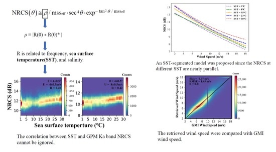
3. Results
3.1. Data Analysis
3.2. Model Design
3.3. Model Validation
4. Discussion
5. Conclusions
Author Contributions
Funding
Institutional Review Board Statement
Informed Consent Statement
Data Availability Statement
Acknowledgments
Conflicts of Interest
References
- Hersbach, H.; Stoffelen, A.; Haan, S.D. An improved C-band scatterometer ocean geophysical model function: CMOD5. J. Geophys. Res. Ocean. 2007, 11, 5767–5780. [Google Scholar] [CrossRef]
- Zhang, B.; Perrie, W.; Vachon, P.W.; Li, X.; Pichel, W.G.; Guo, J.; He, Y. Ocean Vector Winds Retrieval From C-Band Fully Polarimetric SAR Measurements. IEEE Trans. Geosci. Remote Sens. 2012, 50, 4252–4261. [Google Scholar] [CrossRef] [Green Version]
- Freilich, M.H.; Vanhoff, B.A. The Relationship between Winds, Surface Roughness, and Radar Backscatter at Low Incidence Angles from TRMM Precipitation Radar Measurements. J. Atmos. Ocean. Technol. 2003, 20, 549–562. [Google Scholar] [CrossRef]
- Gourrion, J.; Vandemark, D.; Bailey, S.; Chapron, B.; Gommenginger, G. A Two-Parameter Wind Speed Algorithm for Ku-Band Altimeters. J. Atmos. Ocean. Technol. 2002, 19, 2030–2048. [Google Scholar] [CrossRef]
- Hauser, D.; Soussi, E.; Thouvenot, E.; Rey, L. SWIMSAT: A Real-Aperture Radar to Measure Directional Spectra of Ocean Waves from Space—Main Characteristics and Performance Simulation. J. Atmos. Ocean. Technol. 2001, 18, 421–437. [Google Scholar] [CrossRef]
- Barrick, D. Rough Surface Scattering Based on the Specular Point Theory. IEEE Trans. Antennas Propag. 1968, 16, 449–454. [Google Scholar] [CrossRef]
- Jackson, F.C.; Walton, W.T.; Hines, D.E.; Walter, B.A.; Peng, C.Y. Sea surface mean square slope from K u -band backscatter data. J. Geophys. Res. Ocean. 1992, 97, 11411–11427. [Google Scholar] [CrossRef]
- Li, L.; Im, E.; Durden, S.L.; Haddad, Z.S. A Surface Wind Model Based Method to Estimate Rain-Induced Radar Path Attenuation over Ocean. J. Atmos. Ocean. Technol. 2002, 19, 658–672. [Google Scholar] [CrossRef]
- Ngan, T.; Bertrand, C. Combined Wind Vector and Sea State Impact on Ocean Nadir-Viewing Ku- and C-Band Radar Cross-Sections. Sensors 2006, 6, 193–207. [Google Scholar] [CrossRef] [Green Version]
- Tran, N.; Chapron, B.; Vandemark, D. Effect of Long Waves on Ku-Band Ocean Radar Backscatter at Low Incidence Angles Using TRMM and Altimeter Data. IEEE Geosci. Remote Sens. Lett. 2007, 4, 542–546. [Google Scholar] [CrossRef] [Green Version]
- Ren, L.; Yang, J.; Zheng, G.; Wang, J. Wind speed retrieval from Ku-band Tropical Rainfall Mapping Mission precipitation radar data at low incidence angles. J. Appl. Remote Sens. 2016, 10, 016012. [Google Scholar] [CrossRef]
- Bao, Q.; Zhang, Y.; Lang, S.; Lin, M.; Peng, G. Sea Surface Wind Speed Inversion Using the Low Incident NRCS Measured by TRMM Precipitation Radar. IEEE J. Sel. Top. Appl. Earth Obs. Remote Sens. 2016, 9, 5262–5271. [Google Scholar] [CrossRef]
- Panfilova, M.; Karaev, V. Wind Speed Retrieval Algorithm Using Ku-Band Radar Onboard GPM Satellite. Remote Sens. 2021, 13, 4565. [Google Scholar] [CrossRef]
- Chu, X.; He, Y.; Karaev, V.Y. Relationships Between Ku-Band Radar Backscatter and Integrated Wind and Wave Parameters at Low Incidence Angles. IEEE Trans. Geosci. Remote Sens. 2012, 50, 4599–4609. [Google Scholar] [CrossRef]
- Li, X.; Zhang, B.; Mouche, A.; He, Y.; Perrie, W. Ku-Band Sea Surface Radar Backscatter at Low Incidence Angles under Extreme Wind Conditions. Remote Sens. 2017, 9, 474. [Google Scholar] [CrossRef] [Green Version]
- Chu, X.; He, Y.; Chen, G. A new algorithm for wind speed at low incidence angles using TRMM Precipitation Radar data. In Proceedings of the 2010 IEEE International Geoscience & Remote Sensing Symposium, Honolulu, HI, USA, 25–30 July 2010. [Google Scholar] [CrossRef]
- Ren, L.; Yang, J.; Xu, Y.; Zhang, Y.; Zheng, G.; Wang, J.; Dai, J.; Jiang, C. Ocean Surface Wind Speed Dependence and Retrieval From Off-Nadir CFOSAT SWIM Data. Earth Space Sci. 2021, 8, e2020EA001505. [Google Scholar] [CrossRef]
- Vandemark, D.; Chapron, B.; Feng, H.; Mouche, A. Sea Surface Reflectivity Variation With Ocean Temperature at Ka-Band Observed Using Near-Nadir Satellite Radar Data. IEEE Geosci. Remote Sens. Lett. 2016, 13, 510–514. [Google Scholar] [CrossRef]
- Hossan, A.; Jones, W.L. Ku- and Ka-Band Ocean Surface Radar Backscatter Model Functions at Low-Incidence Angles Using Full-Swath GPM DPR Data. Remote Sens. 2021, 13, 1569. [Google Scholar] [CrossRef]
- Panfilova, M.A.; Karaev, V.Y. Evaluation of the boundary wave number for the two-scale model of backscatter of microwaves in Ka- and Ku-band by the sea surface using the Dual-frequency Precipitation Radar data. In Proceedings of the 2016 IEEE International Geoscience and Remote Sensing Symposium (IGARSS), Beijing, China, 10–15 July 2016. [Google Scholar] [CrossRef]
- Bao, Q.; Zhang, Y.; An, W.; Cui, L.; Peng, G. Sea surface wind speed inversion using low incident NRCS. In Proceedings of the IGARSS 2016—2016 IEEE International Geoscience and Remote Sensing Symposium, Beijing, China, 10–15 July 2016. [Google Scholar] [CrossRef]
- Ren, L.; Yang, J.; Jia, Y.; Dong, X.; Wang, J.; Zheng, G. Sea Surface Wind Speed Retrieval and Validation of the Interferometric Imaging Radar Altimeter Aboard the Chinese Tiangong-2 Space Laboratory. IEEE J. Sel. Top. Appl. Earth Obs. Remote Sens. 2018, 11, 4718–4724. [Google Scholar] [CrossRef]
- Yan, Q.; Zhang, J.; Fan, C.; Meng, J. Analysis of Ku- and Ka-Band Sea Surface Backscattering Characteristics at Low-Incidence Angles Based on the GPM Dual-Frequency Precipitation Radar Measurements. Remote Sens. 2019, 11, 754. [Google Scholar] [CrossRef] [Green Version]
- Wang, Z.; Stoffelen, A.; Fois, F.; Verhoef, A.; Zhao, C.; Lin, M.; Chen, G. SST Dependence of Ku- and C-Band Backscatter Measurements. IEEE J. Sel. Top. Appl. Earth Obs. Remote Sens. 2017, 10, 2135–2146. [Google Scholar] [CrossRef]
- Chu, X.; He, Y.; Chen, G. Asymmetry and Anisotropy of Microwave Backscatter at Low Incidence Angles. IEEE Trans. Geosci. Remote Sens. 2012, 50, 4014–4024. [Google Scholar] [CrossRef]
- Stiles, B.W.; Yueh, S.H. Impact of rain on spaceborne Ku-band wind scatterometer data. IEEE Trans. Geosci. Remote Sens. 2002, 40, 1973–1983. [Google Scholar] [CrossRef]
- Weissman, D.E.; Bourassa, M.A. Measurements of the effect of rain-induced sea surface roughness on the satellite scatterometer radar cross section. IEEE Trans. Geosci. Remote Sens. 2008, 46, 2882–2894. [Google Scholar] [CrossRef]
- Portabella, M.; Stoffelen, A.; Lin, W.; Turiel, A.; Verhoef, A.; Verspeek, J.; Ballabrera-Poy, J. Rain Effects on ASCAT-Retrieved Winds: Toward an Improved Quality Control. IEEE Trans. Geosci. Remote Sens. 2012, 50, 2495–2506. [Google Scholar] [CrossRef]
- Lin, W.; Portabella, M.; Zhao, X.; Lang, S. Rain Effects on CFOSAT Scatterometer: Towards an Improved Wind Quality Control. In Proceedings of the IGARSS 2020—2020 IEEE International Geoscience and Remote Sensing Symposium, Waikoloa, HI, USA, 26 September–2 October 2020; pp. 5654–5657. [Google Scholar] [CrossRef]
- Barrick, D.E.; Bahar, E. Rough Surface Scattering Using Specular Point Theory. IEEE Trans. Antennas Propag. 1981, 29, 798–800. [Google Scholar] [CrossRef]
- Weissman, D.E.; Bourassa, M.A. The Influence of Rainfall on Scatterometer Backscatter Within Tropical Cyclone Environments—Implications on Parameterization of Sea-Surface Stress. IEEE Trans. Geosci. Remote Sens. 2011, 49, 4805–4814. [Google Scholar] [CrossRef]
- Contreras, R.F.; Plant, W.J.; Keller, W.C.; Hayes, K.; Nystuen, J. Effects of rain on Ku-band backscatter from the ocean. J. Geophys. Res. Ocean. 2003, 108. [Google Scholar] [CrossRef]
- Ren, L.; Yang, J.; Zheng, G.; Wang, J. A Ku-band wind and rain backscatter model at low-incidence angles using Tropical Rainfall Mapping Mission precipitation radar data. Int. J. Remote Sens. 2017, 38, 1388–1403. [Google Scholar] [CrossRef]


| SST | |||||||||
|---|---|---|---|---|---|---|---|---|---|
| 1 °C | 15.2450 | −0.2689 | −0.0502 | −0.6468 | 0.0351 | 0.0034 | 0.0125 | −0.0012 | −0.00009 |
| 8 °C | 15.8462 | −0.3166 | −0.0488 | −0.7088 | 0.0434 | 0.0032 | 0.0149 | −0.0015 | −0.00009 |
| 15 °C | 16.2395 | −0.3393 | −0.0495 | −0.7403 | 0.0457 | 0.0034 | 0.0160 | −0.0015 | −0.00010 |
| 23 °C | 17.1693 | −0.4589 | −0.0451 | −0.8603 | 0.0683 | 0.0030 | 0.0210 | −0.0025 | −0.00004 |
| 30 °C | 17.1002 | −0.3880 | −0.0498 | −0.8456 | 0.0566 | 0.0032 | 0.0206 | −0.0022 | −0.00004 |
| Coefficient | |||||||||
|---|---|---|---|---|---|---|---|---|---|
| value | 18.5516 | −0.7857 | −0.0452 | −1.1900 | 0.1429 | 0.0023 | 0.0353 | −0.0061 | −0.00004 |
Publisher’s Note: MDPI stays neutral with regard to jurisdictional claims in published maps and institutional affiliations. |
© 2022 by the authors. Licensee MDPI, Basel, Switzerland. This article is an open access article distributed under the terms and conditions of the Creative Commons Attribution (CC BY) license (https://creativecommons.org/licenses/by/4.0/).
Share and Cite
Jiang, C.; Ren, L.; Yang, J.; Xu, Q.; Dai, J. Wind Speed Retrieval Using Global Precipitation Measurement Dual-Frequency Precipitation Radar Ka-Band Data at Low Incidence Angles. Remote Sens. 2022, 14, 1454. https://doi.org/10.3390/rs14061454
Jiang C, Ren L, Yang J, Xu Q, Dai J. Wind Speed Retrieval Using Global Precipitation Measurement Dual-Frequency Precipitation Radar Ka-Band Data at Low Incidence Angles. Remote Sensing. 2022; 14(6):1454. https://doi.org/10.3390/rs14061454
Chicago/Turabian StyleJiang, Chong, Lin Ren, Jingsong Yang, Qing Xu, and Jinyuan Dai. 2022. "Wind Speed Retrieval Using Global Precipitation Measurement Dual-Frequency Precipitation Radar Ka-Band Data at Low Incidence Angles" Remote Sensing 14, no. 6: 1454. https://doi.org/10.3390/rs14061454