
Fast Registration of Terrestrial LiDAR Point Clouds Based on Gaussian-Weighting Projected Image Matching


Abstract
:1. Introduction
1.1. Background
- (1)
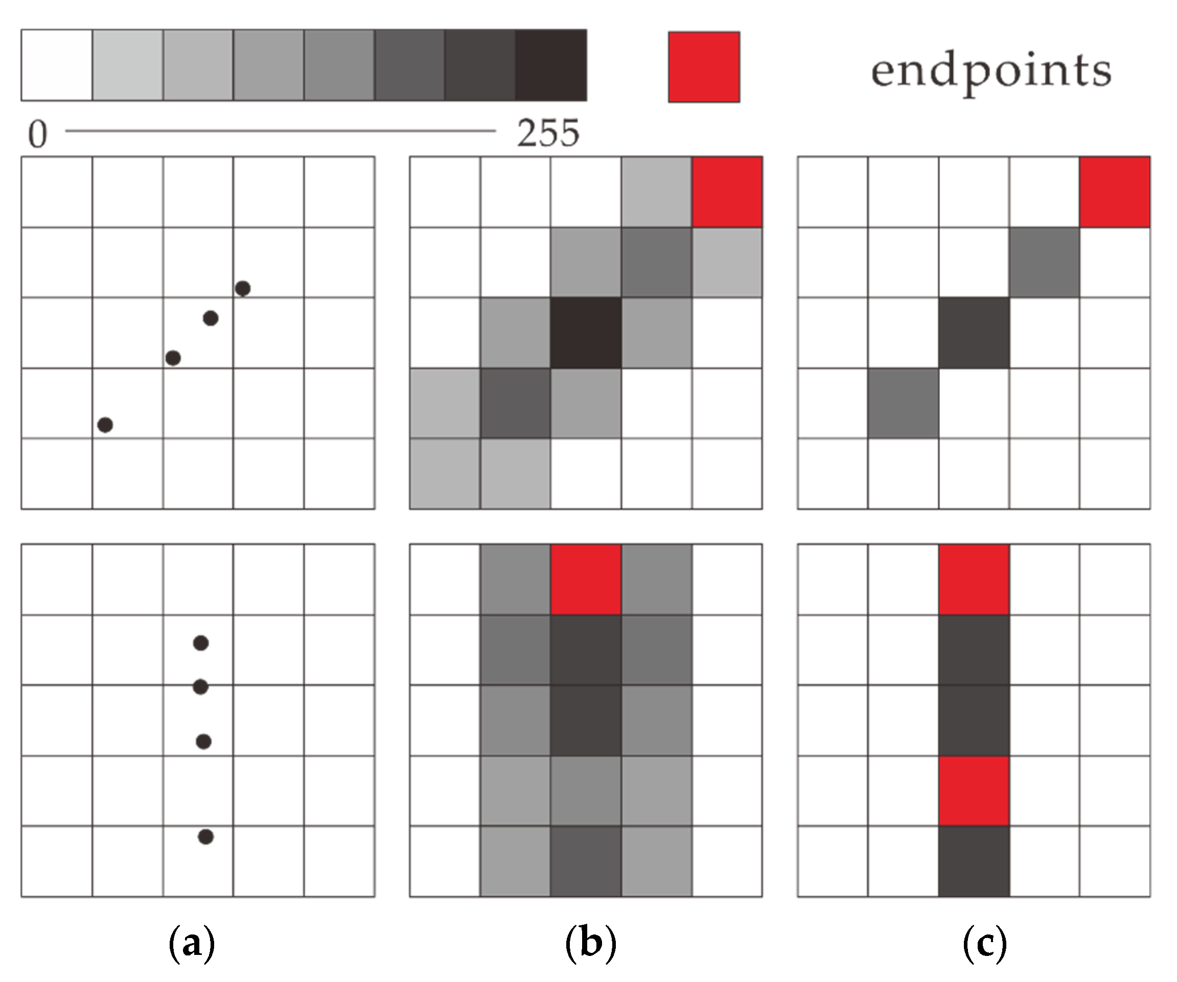
- A Gaussian-weighting projection method is proposed to convert point clouds into grayscale images while preserving salient structural information of the point clouds.
- (2)
- To filter out the negative matches between images, an algorithm is proposed to validate image matching results by extracted line segment endpoints.
1.2. Related Work
2. Materials and Methods
2.1. Gaussian-Weighting Projection
2.2. Endpoint Validated Image Matching
2.2.1. RANSAC Image Matching
| Algorithm 1. RANSAC Image Matching. |
| 1: Macth (Itarget, Isource) |
| 2: SIFT (Itarget, Isource) →n pairs of feature points(Ftarget, Fsource) |
| 3: if (n < 2) return false |
| 4: random (i, j∈[1,n], i≠j) |
| 5: p1 = Ftarget.i, p2 = Ftarget.j |
| 6: p3 = Fsource.i, p4 = Fsource.j |
| 7: Trans |
| 8: RIM = rotation matrix (angle(, )) |
| 9: p3’ = RIM (p3), p4’ = RIM (p4) |
| 10: TIM = dist (midpoint (p1, p2), midpoint (p3’, p4’)) |
| 11: Ts,t ← (RIM, TIM) |
| 12: m = num of dist (Ftarget, Ts,t (Fsource)) < threshold |
| 13: until mmax |
| 14: return Tfinal |
2.2.2. Endpoint Validation
| Algorithm 2. NMS Line Filtering. |
| 1: Filter (parallel lines) |
| 2: collection LA (parallel lines), LF (empty) |
| 3: repeat |
| 4: l = higest voting score(LA) |
| 5: LA.remove(l), LF.add(l) |
| 6: for(l’∈LA) |
| 7: if(dist(l,l’) < threshold) LA.remove(l’) |
| 8: until LA is empty |
| 9: return LF |
2.3. Point Cloud Transformation
2.4. Global Least-Square Optimization
3. Results
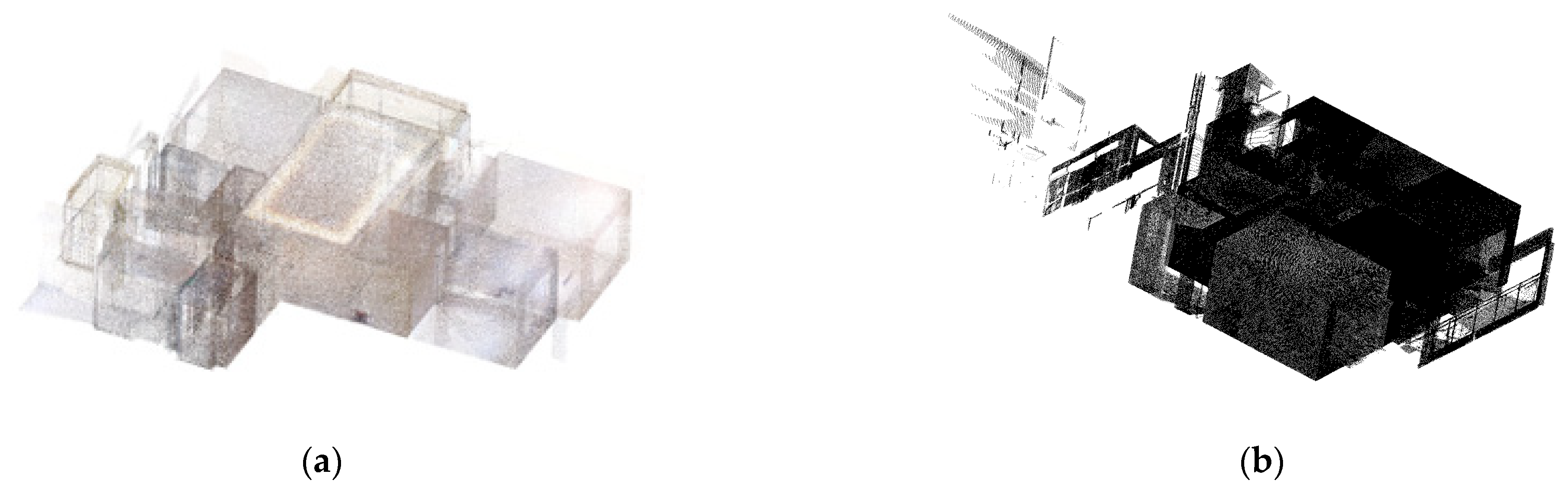
3.1. Dataset
3.2. Evaluation Metrics
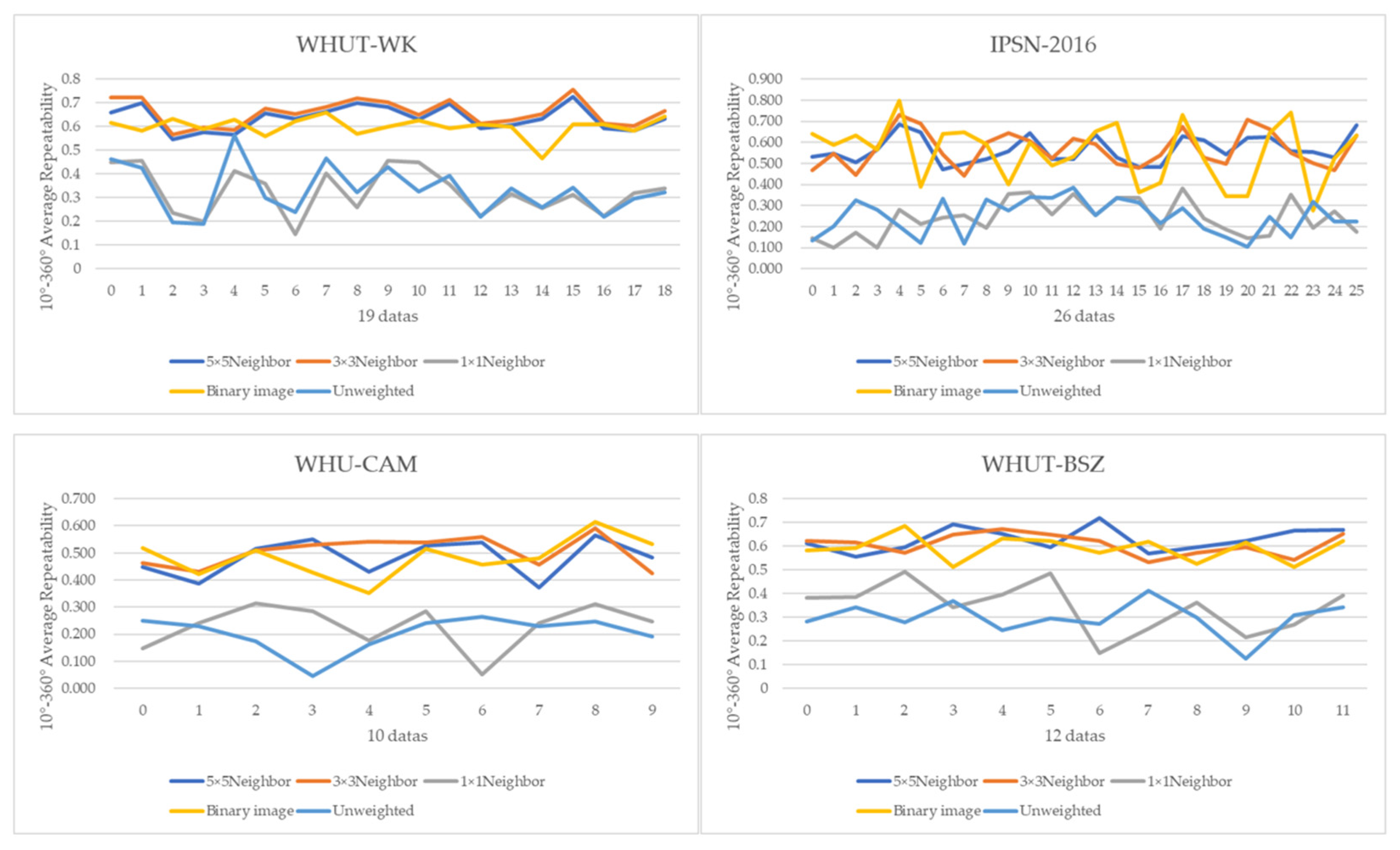
3.2.1. Rotation Invariance of Gaussian-Weighting Projection
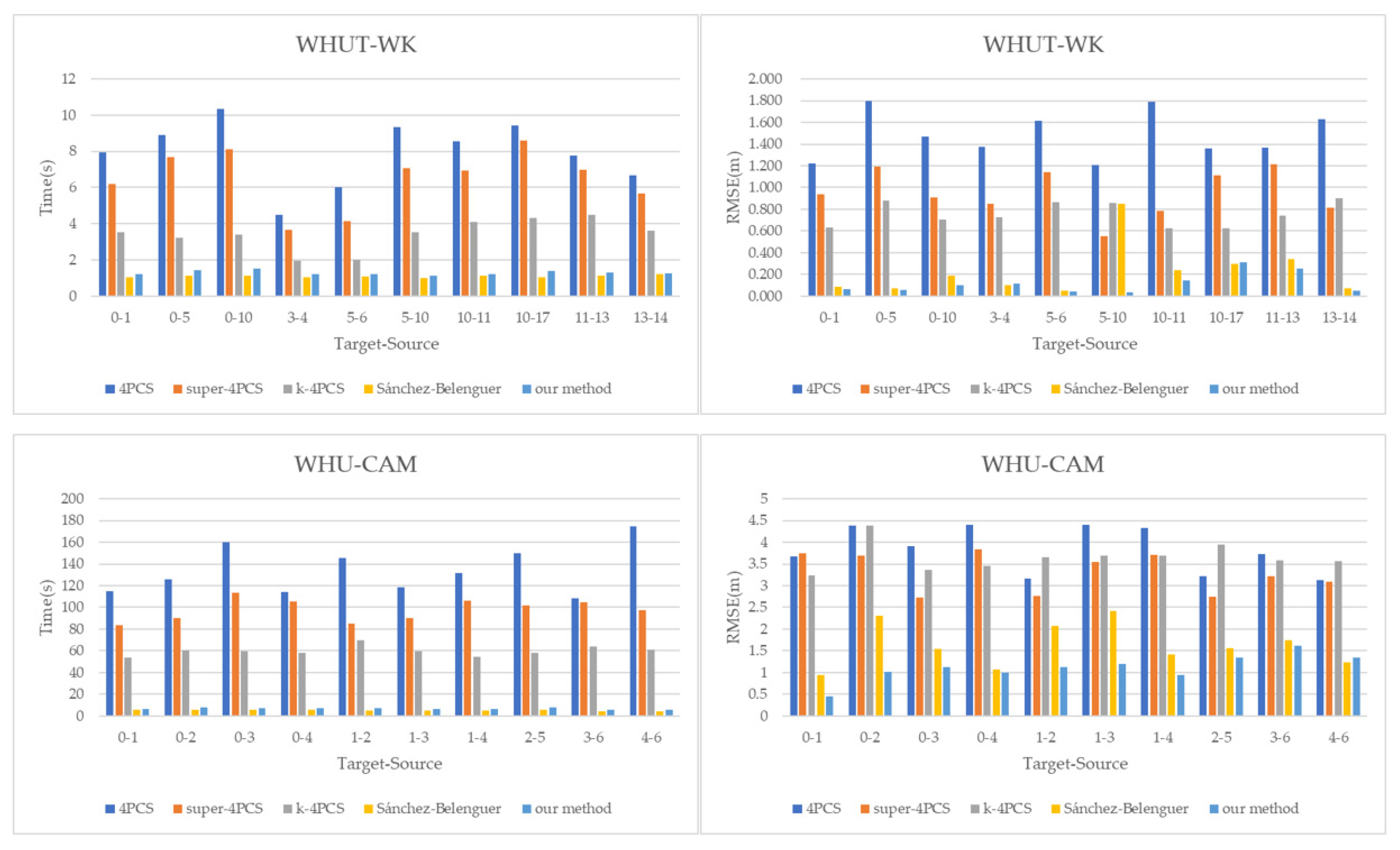
3.2.2. Accuracy and Efficiency of Point Cloud Registration
3.3. Parameter Analysis
3.4. Performance Analysis
3.4.1. Superiority Gaussian-Weighting Projection
3.4.2. Two-Station Cloud Alignment Performance
3.5. Ablation Study
4. Discussion
5. Conclusions
Author Contributions
Funding
Data Availability Statement
Acknowledgments
Conflicts of Interest
References
- Tam, G.K.; Cheng, Z.Q.; Lai, Y.K.; Langbein, F.C.; Liu, Y.; Marshall, D.; Martin, R.R.; Sun, X.F.; Rosin, P.L. Registration of 3D point clouds and meshes: A survey from rigid to nonrigid. IEEE Trans. Vis. Comput. Graph. 2012, 19, 1199–1217. [Google Scholar] [CrossRef] [PubMed] [Green Version]
- Akca, D. Full Automatic Registration of Laser Scanner Points Clouds. Ph.D. Thesis, ETH Zurich, Zurich, Switzerland, 2003. [Google Scholar]
- Al-Durgham, K.; Habib, A.; Kwak, E. RANSAC approach for automated registration of terrestrial laser scans using linear features. In Proceedings of the ISPRS Annals of the Photogrammetry, Remote Sensing and Spatial Information Sciences, Antalya, Turkey, 11–13 November 2013. [Google Scholar]
- Kang, Z.; Li, J.; Zhang, L.; Zhao, Q.; Zlatanova, S. Automatic registration of terrestrial laser scanning point clouds using panoramic reflectance images. Sensors 2009, 9, 2621–2646. [Google Scholar] [CrossRef] [PubMed] [Green Version]
- Kawashima, K.; Yamanishi, S.; Kanai, S.; Date, H. Finding the next-best scanner position for as-built modelling of piping systems. In Proceedings of the International Archives of Photogrammetry, Remote Sensing and Spatial Information Sciences, Riva Del Garda, Italy, 23–25 June 2014. [Google Scholar]
- Besl, P.J.; McKay, N.D. A method for registration of 3-D shapes. IEEE Trans. Patt. Anal. Mach. Intell. 1992, 14, 239–256. [Google Scholar] [CrossRef]
- Frome, A.; Huber, D.; Kolluri, R.; Bülow, T.; Malik, J. Recognizing objects in range data using regional point descriptors. In Proceedings of the European Conference on Computer Vision, Prague, Czech Republic, 11–14 May 2004. [Google Scholar]
- Rusu, R.B.; Blodow, N.; Marton, Z.C.; Beetz, M. Aligning point cloud views using persistent feature histograms. In Proceedings of the IEEE/RSJ International Conference on Intelligent Robots and Systems, Nice, France, 22–26 September 2008. [Google Scholar]
- Rusu, R.B.; Blodow, N.; Beetz, M. Fast point feature histograms (FPFH) for 3D registration. In Proceedings of the IEEE International Conference on Robotics and Automation, Kobe, Japan, 12–17 May 2009. [Google Scholar]
- Rusu, R.B.; Bradski, G.; Thibaux, R.; Hsu, J. Fast 3d recognition and pose using the viewpoint feature histogram. In Proceedings of the IEEE/RSJ International Conference on Intelligent Robots and Systems, Taipei, Taiwan, 18–22 October 2010. [Google Scholar]
- Aiger, D.; Mitra, N.J.; Cohen-Or, D. 4-Points Congruent Sets for Robust Pairwise Surface Registration; ACM: New York, NY, USA, 2008; p. 85. [Google Scholar]
- Mellado, N.; Aiger, D.; Mitra, N.J. Super 4pcs fast global pointcloud registration via smart indexing. Comput. Graph. Forum. 2014, 33, 205–215. [Google Scholar] [CrossRef] [Green Version]
- Mohamad, M.; Rappaport, D.; Greenspan, M. Generalized 4-points congruent sets for 3d registration. In Proceedings of the 2014 International Conference on 3D Vision, Tokyo, Japan, 8–11 December 2014. [Google Scholar]
- Theiler, P.W.; Wegner, J.D.; Schindler, K. Markerless point cloud registration with keypoint-based 4-points congruent sets. In Proceedings of the ISPRS Annals of the Photogrammetry, Remote Sensing and Spatial Information Sciences, Antalya, Turkey, 11–13 November 2013. [Google Scholar]
- Zhong, Y. Intrinsic shape signatures: A shape descriptor for 3D object recognition. In Proceedings of the IEEE International Conference on Computer Vision Workshops, ICCV Workshops 2009, Kyoto, Japan, 27 September–4 October 2009. [Google Scholar]
- Alshawa, M. ICL: Iterative closest line A novel point cloud registration algorithm based on linear features. Ekscentar 2007, 10, 53–59. [Google Scholar]
- Lindeberg, T. Scale Invariant Feature Transform. Scholarpedia 2012, 7, 10491. [Google Scholar] [CrossRef]
- Lowe, D.G. Distinctive image features from scale-invariant keypoints. Int. J. Comput. Vis. 2004, 60, 91–110. [Google Scholar] [CrossRef]
- Lowe, D.G. Object recognition from local scale-invariant features. In Proceedings of the IEEE International Conference on Computer Vision, Kerkyra, Greece, 20–25 September 1999. [Google Scholar]
- Sipiran, I.; Bustos, B. Harris 3D: A robust extension of the Harris operator for interest point detection on 3D meshes. Vis. Comput. 2011, 27, 963–976. [Google Scholar] [CrossRef]
- Harris, C.; Stephens, M. A combined corner and edge detector. In Proceedings of the Alvey Vision Conference, Manchester, UK, 31 August–2 September 1988. [Google Scholar]
- Yew, Z.J.; Lee, G.H. 3dfeat-net: Weakly supervised local 3d features for point cloud registration. In Proceedings of the European Conference on Computer Vision, Munich, Germany, 8–14 September 2018. [Google Scholar]
- Aoki, Y.; Goforth, H.; Srivatsan, R.A.; Lucey, S. Pointnetlk: Robust & efficient point cloud registration using pointnet. In Proceedings of the IEEE Conference on Computer Vision and Pattern Recognition, Long Beach, CA, USA, 15–20 June 2019. [Google Scholar]
- Qi, C.R.; Yi, L.; Su, H.; Guibas, L.J. PointNet++: Deep Hierarchical Feature Learning on Point Sets in a Metric Space. In Proceedings of the Advances in Neural Information Processing Systems, Long Beach, CA, USA, 4–9 December 2017. [Google Scholar]
- Wu, W.; Zhang, Y.; Wang, D.; Lei, Y. SK-Net: Deep learning on point cloud via end-to-end discovery of spatial keypoints. In Proceedings of the AAAI Conference on Artificial Intelligence, New York, NY, USA, 7–12 February 2017. [Google Scholar]
- Wang, Y.; Solomon, J.M. Deep closest point: Learning representations for point cloud registration. In Proceedings of the IEEE/CVF International Conference on Computer Vision, Seoul, Korea, 27 October–2 November 2019. [Google Scholar]
- Xiao, J.; Adler, B.; Zhang, H. 3D point cloud registration based on planar surfaces. In Proceedings of the IEEE International Conference on Multisensor Fusion and Integration for Intelligent Systems, Hamburg, Germany, 13–15 September 2012. [Google Scholar]
- Forstner, W.; Khoshelham, K. Efficient and accurate registration of point clouds with plane to plane correspondences. In Proceedings of the IEEE International Conference on Computer Vision Workshops, Venice, Italy, 22–29 October 2017. [Google Scholar]
- Xiao, J.; Adler, B.; Zhang, J.; Zhang, H. Planar Segment Based Three-dimensional Point Cloud Registration in Outdoor Environments. J. Field Robot. 2013, 30, 552–582. [Google Scholar] [CrossRef]
- Xu, Y.; Boerner, R.; Yao, W.; Hoegner, L.; Stilla, U. Pairwise coarse registration of point clouds in urban scenes using voxel-based 4-planes congruent sets. ISPRS J. Photogramm. Remote Sens. 2019, 151, 106–123. [Google Scholar] [CrossRef]
- Yang, B.; Dong, Z.; Liang, F.; Liu, Y. Automatic registration of large-scale urban scene point clouds based on semantic feature points. ISPRS J. Photogramm. Remote Sens. 2016, 113, 43–58. [Google Scholar] [CrossRef]
- Sumi, T.; Date, H.; Kanai, S. Multiple TLS point cloud registration based on point projection images. In Proceedings of the International Archives of Photogrammetry, Remote Sensing and Spatial Information Sciences, Riva del Garda, Italy, 4–7 June 2018. [Google Scholar]
- Sánchez-Belenguer, C.; Ceriani, S.; Taddei, P.; Wolfart, E.; Sequeira, V. Global matching of point clouds for scan registration and loop detection. Rob. Auton. Syst. 2020, 123, 103324. [Google Scholar] [CrossRef]
- Shi, J. Good Features to Track. In Proceedings of the IEEE Conference on Computer Vision Pattern Recognition, Seattle, WA, USA, 21–23 June 1994. [Google Scholar]
- Li, Z.; Zhang, X.; Tan, J.; Liu, H. Pairwise Coarse Registration of Indoor Point Clouds Using 2D Line Features. ISPRS Int. J. Geo-Inf. 2021, 10, 26. [Google Scholar] [CrossRef]
- Wang, Y.; Zheng, N.; Bian, Z. A Closed-Form Solution to Planar Feature-Based Registration of LiDAR Point Clouds. ISPRS Int. J. Geo-Inf. 2021, 10, 435. [Google Scholar] [CrossRef]
- Ge, X.; Hu, H. Object-based incremental registration of terrestrial point clouds in an urban environment. ISPRS J. Photogramm. Remote Sens. 2020, 161, 218–232. [Google Scholar] [CrossRef]
- Dong, Z.; Liang, F.; Yang, B.; Xu, Y.; Zang, Y.; Li, J.; Wang, Y.; Dai, W.; Fan, H.; Hyyppä, J.; et al. Registration of large-scale terrestrial laser scanner point clouds: A review and benchmark. ISPRS J. Photogramm. Remote Sens. 2020, 163, 327–342. [Google Scholar] [CrossRef]


| Method | 5 × 5 Neighbor | 3 × 3 Neighbor | 1 × 1 Neighbor | Binary Image | Unweighted | |
|---|---|---|---|---|---|---|
| Datasets | ||||||
| WHUT-WK(avg) | 0.635 | 0.658 | 0.325 | 0.600 | 0.332 | |
| WHUT-BSZ(avg) | 0.625 | 0.604 | 0.339 | 0.589 | 0.294 | |
| IPSN-2016(avg) | 0.565 | 0.568 | 0.241 | 0.553 | 0.246 | |
| WHU-CAM (avg) | 0.481 | 0.504 | 0.230 | 0.483 | 0.192 | |
| AVG of all datasets | 0.577 | 0.584 | 0.284 | 0.556 | 0.266 | |
| Datasets (Number of Stations) | Average Error (m)/Number of Alignment Stations | |||
|---|---|---|---|---|
| NGO + NEV | NGO + EV | GO + NEV | GO + EV | |
| WHUT-WK (19) | 5.35/19 | 0.06/10 | 4.21/19 | 0.04/10 |
| WHUT-BSZ (12) | 0.10/12 | 0.10/12 | 0.09/12 | 0.09/12 |
| IPSN-2016 (26) | 3.30/24 | 0.11/21 | 2.61/24 | 0.08/21 |
| IPSN-2017 (47) | 1.86/47 | 1.23/43 | 1.57/47 | 0.98/43 |
| WHU-CAM (10) | 1.08/10 | 1.08/10 | 1.04/10 | 1.04/10 |
| WHU-RES (7) | 0.25/6 | 0.25/6 | 0.23/6 | 0.23/6 |
Publisher’s Note: MDPI stays neutral with regard to jurisdictional claims in published maps and institutional affiliations. |
© 2022 by the authors. Licensee MDPI, Basel, Switzerland. This article is an open access article distributed under the terms and conditions of the Creative Commons Attribution (CC BY) license (https://creativecommons.org/licenses/by/4.0/).
Share and Cite
Xiong, B.; Li, D.; Zhou, Z.; Li, F. Fast Registration of Terrestrial LiDAR Point Clouds Based on Gaussian-Weighting Projected Image Matching. Remote Sens. 2022, 14, 1466. https://doi.org/10.3390/rs14061466
Xiong B, Li D, Zhou Z, Li F. Fast Registration of Terrestrial LiDAR Point Clouds Based on Gaussian-Weighting Projected Image Matching. Remote Sensing. 2022; 14(6):1466. https://doi.org/10.3390/rs14061466
Chicago/Turabian StyleXiong, Biao, Dengke Li, Zhize Zhou, and Fashuai Li. 2022. "Fast Registration of Terrestrial LiDAR Point Clouds Based on Gaussian-Weighting Projected Image Matching" Remote Sensing 14, no. 6: 1466. https://doi.org/10.3390/rs14061466