Prediction of Field-Scale Wheat Yield Using Machine Learning Method and Multi-Spectral UAV Data

Abstract

Accurate prediction of food crop yield is of great significance for global food security and regional trade stability. Since remote sensing data collected from unmanned aerial vehicle (UAV) platforms have the features of flexibility and high resolution, these data can be used as samples to develop regional regression models for accurate prediction of crop yield at a field scale. The primary objective of this study was to construct regional prediction models for winter wheat yield based on multi-spectral UAV data and machine learning methods. Six machine learning methods including Gaussian process regression (GPR), support vector machine regression (SVR) and random forest regression (RFR) were used for the construction of the yield prediction models. Ten vegetation indices (VIs) extracted from canopy spectral images of winter wheat acquired from a multi-spectral UAV at five key growth stages in Xuzhou City, Jiangsu Province, China in 2021 were selected as the variables of the models. In addition, in situ measurements of wheat yield were obtained in a destructive sampling manner for prediction algorithm modeling and validation. Prediction results of single growth stages showed that the optimal model was GPR constructed from extremely strong correlated VIs (ESCVIs) at the filling stage (R² = 0.87, RMSE = 49.22 g/m², MAE = 42.74 g/m²). The results of multiple stages showed GPR achieved the highest accuracy (R² = 0.88, RMSE = 49.18 g/m², MAE = 42.57 g/m²) when the ESCVIs of the flowering and filling stages were used. Larger sampling plots were adopted to verify the accuracy of yield prediction; the results indicated that the GPR model has strong adaptability at different scales. These findings suggest that using machine learning methods and multi-spectral UAV data can accurately predict crop yield at the field scale and deliver a valuable application reference for farm-scale field crop management.

1. Introduction

Accurate prediction of grain crop yield is of great value for the formulation of food policies, the regulation of food prices and agricultural management, and is urgently needed for the development of precision agriculture [1]. Small and medium-sized farms are widely distributed in the world, accounting for more than 80% of global farms, and their food security cannot be guaranteed [2]. Predicting crop yields at small and medium-sized plots can help agricultural producers locate in advance target areas where crop yields are low due to abnormal crop health and low soil fertility. To enable early intervention measures to be taken, precise fertilization and management are required, which represents an effective way to maintain the normal level of crop yield and ensure food security [3]. The traditional method of predicting yield is primarily through field investigation, which is inefficient and even destructive to crops. With the diversity of remote sensing platforms and improvement in the spatial resolution of images, remote sensing techniques have been considered as effective methods for the monitoring of crop growth [4,5]. At present, satellite remote sensing technology is widely used in large-scale agricultural monitoring [6], but it has some shortcomings, such as long revisit periods, coarse resolution and ability to operate in limited meteorological conditions [7,8]. Low-altitude unmanned aerial vehicle (UAV) remote sensing has the advantages of improved spatio-temporal resolution, low operation cost, flexibility and repeatability [9,10]. It can quickly and efficiently acquire centimeter-level remote sensing images of large areas of farmland and effectively assist agricultural operators in management and decision making [11].

Currently, the three typical optical sensors commonly carried by UAV platforms are RGB, multispectral and hyperspectral sensors. RGB cameras are low-cost, but the number of bands is small, and it is difficult to capture complex information contained in the spectrum of the crop canopy [12]. Although hyperspectral sensors have outstanding performance in the high precision characterization of spectral response, they are expensive and involve complicated data processing [13]. Multi-spectral sensors have recently attracted extensive attention from the agricultural quantitative remote sensing community because they are more economical and contain red edge and near-infrared bands, which are important for the estimation of agricultural parameters [14]. The band wavelength of multispectral imaging equipment is generally between 400 and 900 nm, mainly including blue, green, red, red edge and near-infrared. Different vegetation indices (VIs) obtained from different bands have been widely used to determine the values of crop biophysical parameters, which can accurately reflect details of crop growth and the response of the crop to stress (e.g., pests, diseases, temperature, soil, water, etc.) [10]. Many researchers have estimated crop physical and chemical parameters, as well as yield, based on VIs extracted from UAV multi-spectral images, which have achieved good results [15,16,17].

For crop yield prediction, several methods, including process-oriented crop growth models and empirical statistical models [18,19], have recently been developed. Process-oriented crop models are also used to simulate and predict production around the world, such as the world food studies (WOFOST) model [20], the decision support system for agrotechnology transfer (DSSAT) [21], and the agricultural production systems simulator (APSIM) [22]. Although these models are effective in simulating crop yield, they rely on a large number of initial input variables with a priori knowledge, such as climate, soil, and hydrology. Moreover, they are hampered by the high cost of time and labor [23,24]. Traditional statistical regression predicts outputs by developing regression equations between meteorological variables (e.g., temperature, precipitation, solar radiation, etc.) and measured output at different times and different spatial scales [25,26]. These regression results clearly show the impact of climatic factors on yield. The factors that affect yield prediction vary, depending on geographic location, crop varieties and growing seasons [23].

As an immediate successor to statistical regression, machine learning can be used to analyze the hierarchical and non-linear relationships between predictor variables and response variables, and usually performs better than traditional linear regression methods regarding goodness of fit [27]. In addition, machine learning can effectively analyze spectral data and identify crop growth information and is widely used in physiological parameter estimation and crop yield prediction [28,29]. Therefore, many researchers have used UAV remote sensing data and machine learning methods to improve the accuracy of crop yield prediction models. For example, Fu et al. constructed prediction models for winter wheat yield using six machine learning methods including partial least squares regression (PLSR), and found that random forest regression (RFR) had the optimal prediction result in a model constructed using a normalized difference vegetation index (NDVI) (R² = 0.78) [30]. Maimaitijiang et al. used five machine learning methods to develop soybean yield prediction models and found that the highest accuracy was obtained for a deep neural network that provided an R² of 0.72 [31].

Currently, the prediction of many crop yields is based on fixed VIs with a single growth stage of crops [13,32]. Hence, the characteristics of crops at different growth stages are not taken into account[33]. According to previous research, a few studies predict crop yield using an optimal combination of some of the VIs of multiple growth stages. Intuitively determining the optimal VI combination of multiple growth stages can better reflect crop growth law and greatly improve the prediction models of crop yield [34,35]. Furthermore, it is often difficult to predict yield at field scale due to limited surface weather observations on small farms [27]. There are few studies on the stability of yield prediction models at different field scales, so it is difficult to ensure the stability of the model in a larger range of yield prediction. Therefore, the accurate prediction of crop yield at a farm field scale is crucial for optimizing the management of large-scale agricultural operations and improving food security [36].

Since wheat is one of the most widely cultivated food crops in the world and has very high economic value [37], winter wheat was selected for investigation in this study. Based on machine learning methods and the VIs extracted from multi-spectral UAV images, field-scale yield prediction models were developed to better suit the study area and surrounding areas, and the accuracies of the prediction models constructed were subsequently evaluated. The main objectives of this study were to: (1) compare the accuracies of the six selected regression models and to identify the optimal model for single growth stages of winter wheat; (2) identify the prediction model constructed by the combination of the VIs at multiple stages that leads to the best accuracy; (3) verify the performance of the optimal prediction model in larger sampling plots, and also to evaluate the effectiveness of the optimal model in predicting winter wheat yield at field scale.

2. Materials and Methods

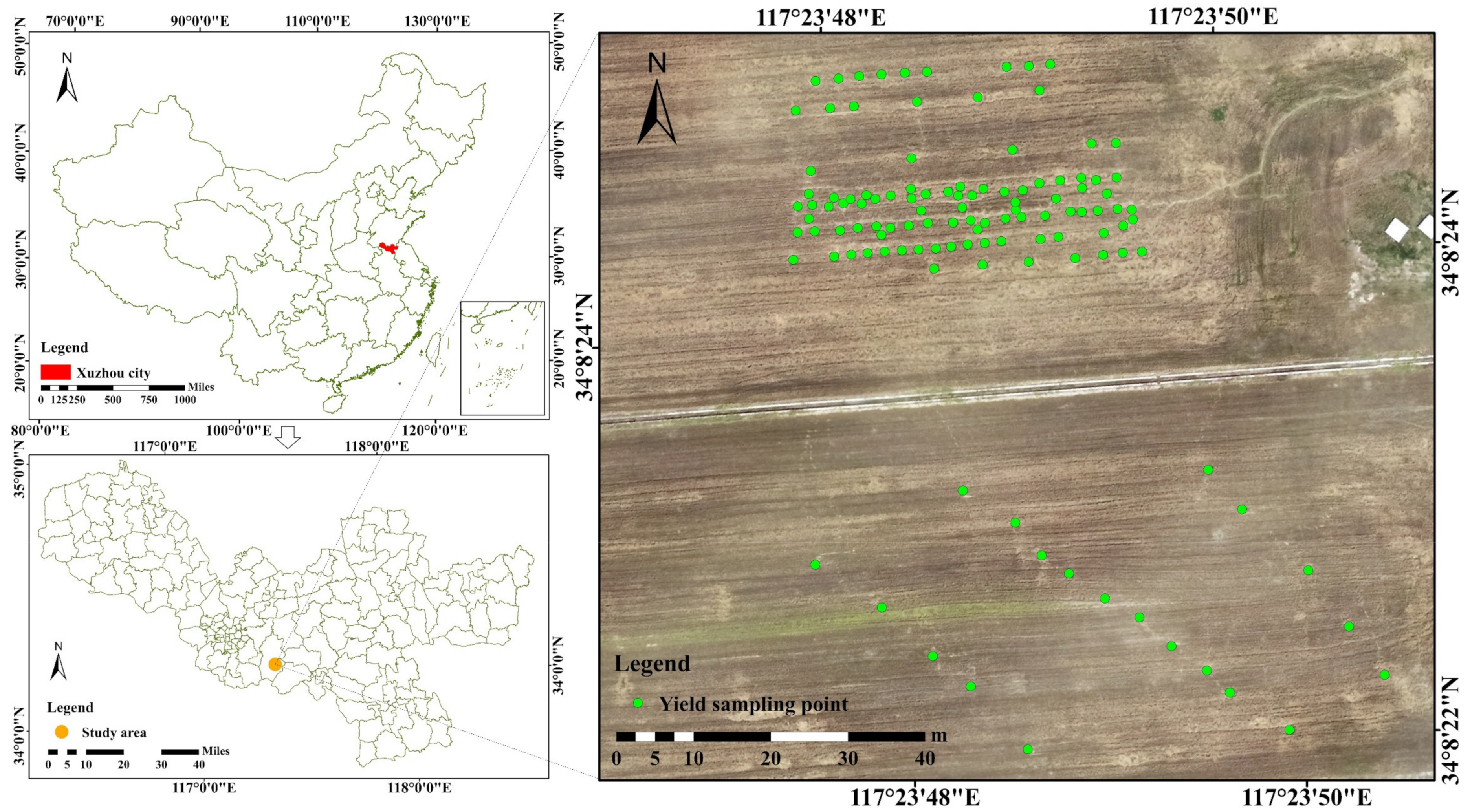
2.1. Study Area

The ground observation experiment was conducted at the Tongshan experimental station (117°23′48″E, 34°8′24″N; Figure 1) in Xuzhou City, Jiangsu province, China. Xuzhou is located in Huang-Huai-Hai Plain, the main winter wheat producing area in China. It is an important grain production base in north China and plays a very important strategic position in China’s grain production pattern. The study area was located in the monsoon climate of medium latitudes, with an average annual temperature of 13.9 °C, an average annual frost-free period of 210 days and average annual precipitation of 868.6 mm. The main soil type in the study area is tidal soil. Note that the main planting structure is the rotation of winter wheat and summer corn. Wheat seeds (Xumai-33) were sown in early October 2020 and the wheat was harvested in early June 2021. An intensive cultivation method was adopted in the study area, and a base fertilizer plus topdressing method was used in fertilization. The basal fertilizer dosage was 1000 kg of organic fertilizer and 30 kg of NPK compound fertilizer (N:P:K = 15:15:15) and 10 kg of urea per mu; the topdressing dosage was 15 kg urea per mu in the middle and late March of 2021.

2.2. Field Data Acquisition

2.2.1. UAV Image Acquisition and Processing

In our experiments, image data were obtained using a multi-rotor UAV (DJI Phantom4 RTK Multispectral) at 100 m altitude with a 5.4 cm spatial resolution (focal length was 5.74 mm, flight speed was 7.5 m/s, the sideways overlap was 60%, the heading overlap was 75%). The UAV images were acquired on 8 April (jointing stage), 19 April (heading stage), 29 April (flowering stage), 20 May (filling stage) and 26 May (milk-ripe stage) in 2021, and the flights were conducted under stable sunlight conditions between 11 a.m. and 1 p.m. The software DJI GS PRO (https://www.dji.com/cn/ground-station-pro/, accessed on 2 June 2021) was used to design the route of the flights and observe the flight status. The multispectral DJI Innovations 4 camera onboard the UAV consisted of an RGB color sensor with a resolution of 1600 × 1300 and five single-band sensors with central wavelengths of 450 ± 16 (blue, B), 560 ± 16 (green, G), 650 ± 16 (red, R), 730 ± 16 (red edge, RE) and 840 ± 26 nm (near-infrared, NIR).

After image data acquisition, the UAV images are required to be preprocessed with image mosaicing and radiometric calibration. The tag image file format (TIFF) images obtained from the UAV were recorded as a set of digital number (DN) values, which needed to be converted into reflectance through radiometric calibration [38]. Before each aerial shooting, the images of a calibration whiteboard (as a reference panel) on the ground were collected for radiometric calibration. Our experiment used the DN values, and the reflectivity of the calibration whiteboard area obtained before the UAV flight, to convert ground DN values into the corresponding reflectivity using the empirical linear correction method [39]. The aerial survey software Pix4Dmapper (Pix4DSA, Co. Ltd., Prilly, Switzerland) was used to complete the radiometric calibration of the multispectral images, and the image mosaic was completed at the same time. Finally, a high-resolution orthophoto of the winter wheat in the study area was obtained.

2.2.2. Yield Data Acquisition

At the mature stage of winter wheat, 119 of 1 m × 1 m quadrats (Figure 1) with uniform growth were randomly selected from the fields in the study area. As shown in Figure 2, all the wheat of the quadrats was harvested (destructive sampling). Moreover, the yield of winter wheat samples was obtained after the processes of threshing, drying to constant weight and weighing (the unit is g/m²). GPS real-time kinematic (RTK) positioning was used to obtain the central position of the sampling squares, and the UAV images of the quadrats region were clipped according to the central position of the quadrats and used to extract the VIs for the modeling of the winter wheat yield.

The frequency distribution of the measured yield data of winter wheat is shown in Figure 3. It can be seen that the spatial heterogeneity of the wheat yield in different quadrats was significant. The lowest and highest yields of the winter wheat samples were 145.9 g/m² and 839.7 g/m², respectively. The values of most of the samples were distributed between 400 and 700 g/m², implying an approximately normal distribution and good representativeness.

2.3. Selection of VIs

It is known that VIs quantitatively indicate crop growth state and can be used for wheat yield prediction [40,41]. In this study, ten VIs obtained from UAV multispectral images were selected to construct winter wheat yield prediction models, and their related information is shown in

Table 1. Selected vegetation indices (VIs) for the yield prediction of the winter wheat.

VI	Formulation	Reference
GRRI	G/R	[44]
GBRI	G/B	[45]
RBRI	R/B	[45]
NDYI	(G − B)/(G + B)	[46]
RVI	NIR/R	[47]
NDVI	(NIR − R)/(NIR + R)	[48]
MTVI	1.2*(1.2*(NIR − G) − 2.5*(R − G))	[49]
EVI2	2.5*(NIR − R)/(NIR + 2.4*R + 1)	[50]
MSAVI2	0.5*((2*NIR + 1) − (sqrt((2*NIR)^2 − 8*(NIR − R))	[51]
TCARI	3*((RE − R) − 0.2*(RE − G)*(RE/R))	[52]

. The ten VIs have been widely used in crop yield prediction [42,43], including green red ratio index (GRRI), green blue ratio index (GBRI), red blue ratio index (RBRI), normalized difference yellowness index (NDYI), NDVI, ratio vegetation index (RVI), modified triangular vegetation index (MTVI), enhanced vegetation index 2 (EVI2), modified soil adjusted vegetation index 2 (MSAVI2) and transformed chlorophyll absorption in reflectance index (TCARI). Each VI value of each quadrat was obtained by substituting the mean reflectivity of each band of the clipped quadrat image into the VI formulation in Table 1.

Each subfigure in Figure 4 shows the variation of each VI extracted from the multispectral images of 119 yield quadrats with the five crop growth stages. It can be seen that the VIs in most of the subfigures (except for the second, third, and fourth subfigures from left to right) showed a gradually decreasing or increasing trend with crop growth, and the VIs at the filling and milky-ripe stages were significantly different from the other stages in the same subfigure. In addition, the VIs at the flowering stage showed a notable difference from the first two stages. These phenomena reflect the changes in crops at different growth stages.

2.4. Machine Learning Methods for Yield Prediction

Six common machine learning algorithms were tested for the identification of the optimal prediction model of wheat yield, including Gaussian process regression (GPR), support vector machine regression (SVR), RFR, decision tree (DT), least absolute shrinkage and selection operator (Lasso), and gradient boost regression tree (GBRT). The hyper-parameters of these models were tuned to improve model accuracy through the GridSearchCV package in Python 3.7.

GPR is a nonlinear regression algorithm conforming to a generalized Gaussian probability distribution [53]. Compared with conventional regression methods, the parameter optimization of GPR is simpler and is often used for regression problems with small samples [54]. In this study, the DotProduct kernel function was applied in the GPR method to construct the yield prediction models. The SVR designs the linear classifier of the maximum decision boundary to ensure the minimum generalization error in the worst case, according to the principle of structural risk minimization [55]. The SVR model uses kernel functions to map the input into a high-dimensional space and then make it linearly separable to balance error minimization and overfitting [25]. In this study, the linear kernel function was applied in the SVR method. The RFR model integrates multiple decision trees through the bagging algorithm idea of ensemble learning, and is suitable for high-dimensional data for feature selection and machine learning [56]. The algorithm is more robust to noise immunity and less prone to overfitting problems [57]. For the RFR model, n_estimators, max_depth, min_samples_split were all optimally adjusted using the GridSearchCV package. Although the DT is a popular and effective modeling algorithm mainly for predicting simple data [58], it can be more easily overfitted compared with the RFR, and provides poor prediction results [59]. The Lasso method obtains a relatively refined model by constructing a penalty function and forcing the sum of the absolute values of some regression coefficients to be within a fixed value and setting some of the other regression coefficients to be zero [60]. Although this method can effectively eliminate significant and high correlation variables, the penalty function may lead to underfitting [27]. The GBRT method is a DT integrated learning algorithm with forward distribution [61]; it builds a new model through the current model and a fitting function to minimize the loss function, thus the accuracy of the model is gradually improved [62,63]. This algorithm can reduce the model learning rate to prevent overfitting, however, the constructed model is sensitive to parameter changes.

2.5. Evaluation Indexes of Models

The procedure followed for the six prediction models for winter wheat yield, constructed based on the ten VIs extracted from UAV multispectral image data and measured yield, is shown by the flowchart in Figure 5. A hold-out method was used to select the training and test samples [64]. All samples were divided into disjoint training and test samples in a ratio of 3:1. At the same time, we used a distribution ratio of training and test samples of roughly 3:1 in different yield intervals, in a similar way to stratified sampling, to avoid the phenomenon of uneven sample distribution. To avoid the influence of an inconsistent order of magnitude of the sample data, all the sample data were standardized before the modeling process started. In this study, the coefficient of determination (R²), root mean square error (RMSE) and mean absolute error (MAE) were selected for the evaluation of the performance of the model, and their formulas are:

$${\mathrm{R}}^2=\frac{\left({{\displaystyle \sum }}_{i=1}^k(y_i-\overline{y}\right)\left(f_i-\overline{f}\right){)}^2}{{{\displaystyle \sum }}_{i=1}^k{\left(y_i-\overline{y}\right)}^2{{\displaystyle \sum }}_{i=1}^k{(f_i-\overline{f})}^2}$$

(1)

$$\mathrm{RMSE}=\sqrt{\frac{1}{k}{\displaystyle \sum }_{i=1}^k{\left(y_i-f_i\right)}^2}$$

(2)

$$\mathrm{MAE}=\frac{1}{k}{\displaystyle \sum }_{i=1}^k\left|y_i-f_i\right|$$

(3)

where i (=1, 2, …, k) is the index of the sample; k is the number of the samples used in the modeling; $y_i$ is the measured winter wheat yield; $\overline{y}$ is the mean of all $y_i$; $f_i$ is the predicted winter wheat yield; $\overline{f}$ is the mean of all $f_i$. The larger the R² value, the higher the accuracy of the model. A small RMSE or MAE value means a small discrepancy between the predicted yield and the measured yield.

3. Results

3.1. Comparison of Model Accuracies at Different Stages

In this study, the measured yield for winter wheat samples (which are mentioned in Section 2.2.2) were taken as the truth of the yield, and the ten VIs at each growth stage were used as the input variables of the selected six regression models. Figure 6 shows the accuracy of the predictions made by these models at each single growth stage. It was found that the results of the GPR model were 0.77 ≤ R² ≤ 0.87, 49.41 g/m² ≤ RMSE ≤ 65.49 g/m² and 42.82 g/m² ≤ MAE ≤ 55.48 g/m². The R², RMSE and MAE values of the SVR and RFR models at the jointing, flowering and filling stages were all larger than 0.72, less than 71.60 g/m² and less than 64.07 g/m², respectively. However, the prediction accuracies of DT, Lasso and GBRT were all low, and the R², RMSE and MAE values at the jointing, heading, flowering and milk-ripe stages were all under 0.71, above 73.40 g/m² and above 63.97 g/m², respectively. These results imply that GPR, SVR and RFR were more suitable for yield prediction than the other three; thus, these three models were considered as the candidates for the identification of the optimal model.

The training results of GPR, SVR and RFR are presented in the form of scatter plots of yield prediction of the models and measured yield at each growth stage, see Figure 7. The plots show good linear fitting between the yield predictions and measurements. The RMSEs and MAEs of the three models were all lower than 78.20 g/m² and 64.07 g/m², respectively, showing high prediction accuracy. Moreover, it was found that GPR outperformed SVR and RFR with respect to comparison of the prediction accuracies of the above three models at the same growth stage. Among the accuracies of the same model at different growth stages, the prediction accuracy at the filling stage was the best.

3.2. Yield Prediction for Multiple Stages

3.2.1. Correlation Analysis

In this section, the Pearson correlation coefficient ($\mathrm{R}$) between each of the ten selected VIs and the yield at each stage is determined, and the correlation is used to identify both the growth stages and the combination of some of the ten VIs that led to the best accuracy. The Pearson correlation coefficient is often used to evaluate the degree of correlation between two variables. Its advantage lies in the averaging of the two variables, which reduces the influence of the numerical difference between the two variables on the similarity of the two variables. The formula of$\mathrm{R}$ between yield and each VI at each growth stage is:

$$\mathrm{R}=\frac{{{\displaystyle \sum }}_{i=1}^k\left(x_i-\overline{x})(y_i-\overline{y}\right)}{\sqrt{{{\displaystyle \sum }}_{i=1}^k{\left(x_i-\overline{x}\right)}^2}\sqrt{{{\displaystyle \sum }}_{i=1}^k{\left(y_i-\overline{y}\right)}^2}}$$

(4)

where i (=1, 2, …, k) is the index of the sample; k is the number of the samples used in the modeling; $x_i$ is the value of the VI at the growth stage; $\overline{x}$ is the mean of all $x_i$;$y_i$ is the measured yield; $\overline{y}$ is the mean of all $y_i$. The closer $\left|R\right|$ is to 1, the stronger the correlation between the VI and the yield. Generally, if the correlation values are in the range 0.8–1.0, 0.6–0.8, 0.4–0.6, 0.2–0.4, and 0.0–0.2, then they are regarded to be an extremely strong correlation, a strong correlation, a moderate correlation, a weak correlation, and a very weak or no correlation, respectively [65].

Figure 8 shows the absolute value of $\mathrm{R}$ between yield and each of the ten VIs at each growth stage. We found that, at the filling stage, the VIs of RBRI, RVI, NDVI, MTVI, EVI2, MSAVI2 and the yield were extremely strong correlated, which can be called extremely strong correlated VIs (ESCVIs). At the flowering stage, RVI, MTVI, EVI2, MSAVI2 were ESCVIs. The VIs of the other three growth stages were mainly moderately or strongly correlated with the yield. It can be concluded that the correlation between each of the VIs and the yield was generally highest at the filling stage, and higher at the flowering stage than the other three stages. This explains why the accuracy of the selected six models at the filling stage was the highest among the five growth stages in Section 3.1. Previous studies have shown that the correlations between each VI and crop yield at the flowering and filling stages are particularly close [66,67], which is consistent with the results in this section.

3.2.2. Yield Prediction for Multiple Stages

To determine the correlation between each VI and crop yield at each growth stage, in this section, the GPR, SVR and RFR methods are used to build yield models for multiple stages and different combinations of the VIs. First, all the VIs at the flowering and filling stages were input into the model training simultaneously. Secondly, the ESCVIs of Section 3.2.1 at either the flowering stage (RVI, MTVI, EVI2, MSAVI2) or the filling stage (RBRI, RVI, NDVI, MTVI, EVI2, MSAVI2) were input into model training. Finally, all the ESCVIs of the two stages were used for the model training. In this experiment, 89 samples were randomly selected for the training phase and the remaining 30 samples were used for the verification phase. The accuracy of the models constructed with two combinations of the VIs at each of the two stages and their merged stages (i.e., flowering and filling stages) are shown in

Table 2. R², RMSE and MAE of the six yield models constructed with different combinations of the VIs at the flowering, filling and flowering and filling stages.

Combination of VIs	All VIs			ESCVIs
Stage\Algorithm	GPR	SVR	RFR	GPR	SVR	RFR
Flowering	0.79 a	0.77 a	0.75 a	0.80 a	0.82 a	0.77 a
	62.60 b	64.34 b	67.66 b	63.46 b	59.26 b	67.07 b
	49.37 c	52.32 c	52.81 c	52.47 c	49.65 c	49.52 c
Filling	0.87 a	0.86 a	0.83 a	0.87 a	0.87 a	0.80 a
	49.41 b	50.55 b	55.51 b	49.22 b	49.33 b	63.12 b
	42.82 c	43.44 c	44.29 c	42.74 c	42.83 c	53.08 c
Flowering & Filling	0.83 a	0.79 a	0.83 a	0.88 a	0.87 a	0.86 a
	58.24 b	63.86 b	56.68 b	49.18 b	50.83 b	52.88 b
	49.77 c	52.56 c	46.36 c	42.57 c	43.34 c	43.42 c

^a represents the value of R², ^b represents the value of RMSE, ^c represents the value of MAE, the unit of RMSE and MAE is g/m²; Flowering & Filling represents the flowering and filling stages considered together; boldface represents the best performance achieved by all yield prediction models.

.

It can be seen from Table 2 that the R², RMSE and MAE values of the GPR, SVR and RFR models were in the range 0.75–0.88, 49.18–67.66 g/m², 42.57–53.08 g/m², respectively. In terms of RMSE and MAE, GPR slightly outperformed SVR at all three stages mentioned in this section. At the flowering stage, SVR effectively improved its performance from R² = 0.77, RMSE = 64.34 g/m² and MAE = 52.32 g/m² to R² = 0.82, RMSE = 59.26 g/m² and MAE = 49.65 g/m² using the ESCVIs (consisting of RVI, MTVI, EVI2, and MSAVI2). Different from the flowering stage, the three models at the filling stage using the ESCVIs (consisting of RBRI, RVI, NDVI, MTVI, EVI2 and MSAVI2) slightly outperformed the models using all the VIs. Moreover, when jointly using VIs at the flowering & filling stages, Table 2 shows that the accuracy of the above three models based on all the VIs was not significantly improved. However, the accuracies of the models based on the ESCVIs were slightly improved at this stage, especially the GPR model (R² = 0.88, RMSE = 49.18 g/m², MAE = 42.57 g/m²) and the RFR model (R² = 0.86, RMSE = 52.88 g/m², MAE = 43.42 g/m²). All the above results imply that the models that were based on the ESCVIs, rather than all the VIs, significantly improved their accuracies at the flowering stage. In addition, the accuracies of the predictions made by the three models were also improved at the filling and flowering & filling stages, but the improvement was insignificant.

3.3. Yield Prediction in Large Plots

To evaluate the adaptability of the optimal model at different scales, ten 3 m × 3 m and seven 5 m × 5 m sampling plots were selected for testing. These plots were in the field shown in Figure 1, and their distribution is shown in Figure 9. To obtain the mean yield of each plot, the three (or five 1 m × 1 m sampling squares) shown in this figure were randomly selected for the sampling of the plot. The mean yield of the three (or five) sampling squares in the plot was used as the reference (or truth) for the yield of the plot. Based on the results presented in Section 3.2 that the GPR model constructed by the ESCVIs at the flowering and filling stages was the optimal model, this model was used to predict the mean yield of winter wheat in each plot; the comparisons between the predicted values and the truth of each plot are shown in

Table 3. Comparison of yield prediction accuracy of the GPR model constructed by combining the ESCVIs at the flowering and filling stages in different sized plots. Boldface represents the best performance.

Plots/Indexes (g/m2)	Mean of Measurements	Mean of Predictions	RMSE	MAE
1 m × 1 m	529.58	532.58	63.44	50.97
3 m × 3 m	554.05	529.72	55.95	38.73
5 m × 5 m	515.83	534.10	39.76	35.48

.

It can be seen from Table 3 that the RMSE of the predicted yields of all the 3 m × 3 m sampling plots was 55.95 g/m², which was smaller than the RMSE of 63.44 g/m² of the 1 m × 1 m sampling squares (see all the green points in Figure 9) by 7.49 g/m². Meanwhile, the MAE of the predicted yields of all the 3 m × 3 m sampling plots was smaller than the MAE of the 1 m × 1 m sampling squares by 12.24 g/m². The yield sampling points in the 5 m × 5 m sampling plots were evenly distributed within the sampling plots, and the RMSE and MAE of the yield prediction were smaller than that of 1 m × 1 m plots by 23.68 g/m² and 15.49 g/m², respectively. The reason is assumed to be that the prediction errors of wheat yield in large sampling plots will cancel each other, which is consistent with previous studies [64]. From Table 3, the difference between the predicted mean yield and the measured mean yield was small, which verifies the strong adaptability of the GPR model constructed by combining the ESCVIs at the flowering and filling stages at different scales.

3.4. Spatial Distribution of Predicted Yield

In this section, the accuracy of the predictions made by the optimal model (i.e., the GPR model constructed by the ESCVIs at the flowering and filling stages) for an area that was expanded from the area covered by the sampling points (in Figure 1) is evaluated. Since the true yield of the expanded area is unknown, the spatial distribution of the predicted yield was compared with that of the UAV orthoimage. Figure 10 shows the results, where a, b, c, d, e, f, and g are the feature areas selected for analysis of their accuracy, and the minimum unit of prediction was 1 m × 1 m. It should be noted that the reason for the selection of the filling stage in (B) is that model accuracy at the filling stage was higher than at the flowering stage.

Comparing (A) and (B) in Figure 10, we found that the spatial characteristics of the yield predictions shown in (A) agree with the (horizontal) line seeding texture of the sowing machine shown in (B), especially in the feature areas b and d. The yield predictions are mainly distributed in the range 400–700 g/m², which is consistent with the measured yields of the region. Those areas where the yield was above 700 g/m² (in orange) were mainly concentrated in the eastern region (areas c, e, and g), while the areas that yielded under 400 g/m² were concentrated in a and f. During the period of sampling, we found that the planting density in the eastern part of the plot was larger than the western part, while the growth in the western part was obviously not as good as in the eastern part. Moreover, bare soil could be directly observed in the f area in Figure 10B. Therefore, the spatial distribution of the predicted yield was roughly consistent with the actual situation.

To some extent, the predicted spatial distribution of yield reflected the yield distribution of winter wheat in farmland. The actual yield of winter wheat was higher in the region with higher yield prediction, which was roughly consistent with the field survey. According to Figure 10, the areas with low yield (area a and f) can be found in advance, associated with insufficient nitrogen application, diseases and insect pests, etc., and prevention and control can be carried out in advance to maintain the normal level of yield and ensure food security.

4. Discussion

Many studies have found that ground spatial heterogeneity and the physiological characteristics of crops vary with crop growth stage [68,69,70]. Figure 6 indicates that the ten selected VIs at different stages may lead to significantly different accuracies of yield predicted by a model, which is consistent with previous studies. The jointing stage is the key growth stage for determining the numbers of panicles and amount of grain, but the VIs at this stage cannot reflect the dry matter accumulation process of yield forming organs, resulting in low prediction accuracy. The filling stage is the stage when starch, protein and other organic matter produced by photosynthesis are transferred from vegetative organs to grains [71]. The VIs at the filling stage directly reflect the final growth state of winter wheat and are closely related to the thousand-grain weight, thus yield prediction accuracy is highest at the filling stage. As can be seen from Figure 7, the R² values for the prediction models constructed by GPR, SVR and RFR machine learning methods at the filling stage were 0.87, 0.86 and 0.83, respectively, showing the highest accuracy among all the stages, which is consistent with previous studies [71,72]. Due to the gradual transfer of nutrients from canopy leaves and stems to grains, chlorophyll content in leaves decreases, and the correlation between the VIs based on red and near-infrared wavelengths and dry matter accumulation in grains decreases, thus the accuracy of the model decreased at the later stage of crops (i.e., the milk-ripe stage)[33].

This study also constructed yield prediction models for the VIs at multiple stages. When all ten VIs were used as the input variables, the accuracy of the models was lower than that of a single stage, which may be caused by the multicollinearity of the input VIs and the low correlation between some of the VIs and the yield. Some studies have also shown that the VIs at all stages have certain errors, thus the accumulated VIs for multiple stages may have accumulated errors in the VI variables, which may decrease model accuracy [73]. It is worth mentioning that in this study, when the ESCVIs at the flowering and filling stages were used as input variables, the yield prediction accuracy was improved to some extent, compared with the same model but at a single stage, which is consistent with previous studies [66,67].

The prediction of wheat yield at the field scale has significant practical significance for wheat production and planting planning. In this study, the spatial resolution of UAV remote sensing data was 5.4 cm, the area size of the sampling square was 1 m², and the growth of wheat in the selected quadrat was relatively uniform. Therefore, the mean of the VIs of the quadrat was adopted for the VIs of the quadrat. It is worth mentioning that 3 m × 3 m and 5 m × 5 m sampling plots have rarely been tested in previous studies. It can be seen from Table 3 that the prediction error will not increase if 1 m² sampling squares fully represent the mean yield of each sampling plot. Thus, the optimal model (i.e., the GPR model constructed by the ESCVIs at the flowering and filling stages) can be applied to the yield predictions at a larger field scale. Previous studies have shown that the larger the spatial scale, the more positive and negative errors of the predictions will be canceled, and the higher the accuracy of the yield predictions [74]. It can be seen that UAV remote sensing data has a high degree of generality, and with increase in field size, the actual yield fluctuates less to a certain extent. Therefore, the yield prediction model has strong adaptability at different field scales, and this study can provide a reference and technical support for farm managers in field management and regulation.

Some uncertainties remain in this study. First, there are uncertainties in data quality, such as GPS RTK recording drift errors in the central position of the sampling squares and artificial harvesting and these measurement errors potentially create uncertainties in yield prediction. Second, different varieties of wheat have different dry matter accumulation [75], and their nitrogen accumulation in grains and various vegetative organs is also different [76]. The accuracy of the yield prediction model may change due to the different accumulation of dry matter and nitrogen. Therefore, yield prediction for different varieties of wheat can be studied in the future. Third, crop yields are affected by many factors, such as climate factors (e.g., temperature, rainfall, light, etc.), soil properties (e.g., PH, organic matter, humidity, etc.), and human management practices (e.g., fertilization, irrigation, pesticides) [77]. Due to small differences in variables at the field scale, this study has not considered these variables for the time being. However, these variables need to be considered in subsequent predictions of crop yield at a larger scale. For example, Han et al. used VIs, climate, soil and other variables to predict the county-level winter wheat yield in various agricultural regions in China [78]. In terms of research scale, the transition from field scale to regional scale should be gradually effected to achieve efficient, high-precision and large-scale crop yield prediction [79].

5. Conclusions

In this study, VIs extracted from multi-spectral UAV data and machine learning methods were used to construct six regression models or algorithms for the prediction of winter wheat yield at the field scale. The results showed that the yield prediction model established at the filling stage outperformed other single-stage models. They also showed that the yield prediction model established at the single stage by GPR, SVR and RFR showed better performance compared with the other three algorithms, among which the GPR model could predict the winter wheat yield more accurately before harvest. The GPR, SVR and RFR models for different stages and from the input of different combinations of some of the VIs were developed and compared. It was found that the optimal yield prediction model of a single stage was established by the ESCVIs of the filling stage. This result showed that if only one observation was provided in the predicted yield area, the best observation time was at the filling stage. Moreover, the GPR model combined with the ESCVIs at the flowering and filling stages was the best performer, i.e., the optimal model. This indicates that, if the yield prediction area can be observed many times, the model combined with the ESCVIs at the flowering and filling stages can improve the accuracy. Furthermore, the optimal model was tested using its predicted yield of large plots compared with the yield measurements, and we found that the optimal model had strong adaptability at different scales. The spatial distribution of wheat yield predicted by the optimal model for the fields studied was also compared with the reference of the UAV orthoimage and the predicted result was found to be reliable.

As indicated above, this study provides a reference and technical support for field management and decision making in small and medium-sized planting areas. However, there is still much to explore in crop yield prediction at the field scale. Regarding the limitations of this study, future work will focus on the following: (1) increasing samples of measured yield data to improve model accuracy and stability; (2) combining more types of crop physiological parameters to improve model accuracy; (3) establishing a cross-regional model to verify the universal applicability of the model; and (4) exploring a combination with satellite imagery to predict crop yield over a wide region possible.

References

1. Mueller, N.D.; Gerber, J.S.; Johnston, M.; Ray, D.K.; Ramankutty, N.; Foley, J.A. Closing yield gaps through nutrient and water management. Nature 2012, 490, 254–257. [Google Scholar] [CrossRef] [PubMed]
2. Samberg, L.H.; Gerber, J.S.; Ramankutty, N.; Herrero, M.; West, P.C. Subnational distribution of average farm size and smallholder contributions to global food production. Environ. Res. Lett. 2016, 11, 124010. [Google Scholar] [CrossRef]
3. Bongiovanni, R.; Lowenberg-Deboer, J. Precision Agriculture and Sustainability. Precis. Agric. 2004, 5, 359–387. [Google Scholar] [CrossRef]
4. Fu, Y.; Yang, G.; Wang, J.; Song, X.; Feng, H. Winter wheat biomass estimation based on spectral indices, band depth analysis and partial least squares regression using hyperspectral measurements. Comput. Electron. Agric. 2014, 100, 51–59. [Google Scholar] [CrossRef]
5. Wang, Y.; Chang, K.; Chen, R.; Lo, J.; Shen, Y. Large-area rice yield forecasting using satellite imageries. Int. J. Appl. Earth Obs. 2010, 12, 27–35. [Google Scholar] [CrossRef]
6. Du, M.; Noguchi, N. Multi-temporal monitoring of wheat growth through correlation analysis of satellite images, unmanned aerial vehicle images with ground variable. IFAC-PapersOnLine 2016, 49, 5–9. [Google Scholar] [CrossRef]
7. Berni, J.A.J.; Zarco-Tejada, P.J.; Suarez, L.; Fereres, E. Thermal and narrowband multispectral remote sensing for vegetation monitoring from an unmanned aerial vehicle. IEEE Trans. Geosci. Remote 2009, 47, 722–738. [Google Scholar] [CrossRef] [Green Version]
8. Yu, N.; Li, L.; Schmitz, N.; Tiaz, L.F.; Greenberg, J.A.; Diers, B.W. Development of methods to improve soybean yield estimation and predict plant maturity with an unmanned aerial vehicle based platform. Remote Sens. Environ. 2016, 187, 91–101. [Google Scholar] [CrossRef]
9. Zhang, C.; Kovacs, J.M. The application of small unmanned aerial systems for precision agriculture: A review. Precis. Agric. 2012, 13, 693–712. [Google Scholar] [CrossRef]
10. Verger, A.; Vigneau, N.; Cheron, C.; Gilliot, J.; Comar, A.; Baret, F. Green area index from an unmanned aerial system over wheat and rapeseed crops. Remote Sens. Environ. 2014, 152, 654–664. [Google Scholar] [CrossRef]
11. Candiago, S.; Remondino, F.; De Giglio, M.; Dubbini, M.; Gattelli, M. Evaluating multispectral images and vegetation indices for precision farming applications from UAV images. Remote Sens. 2015, 7, 4026–4047. [Google Scholar] [CrossRef] [Green Version]
12. Bendig, J.; Yu, K.; Aasen, H.; Bolten, A.; Bennertz, S.; Broscheit, J.; Gnyp, M.L.; Bareth, G. Combining UAV-based plant height from crop surface models, visible, and near infrared vegetation indices for biomass monitoring in barley. Int. J. Appl. Earth Obs. 2015, 39, 79–87. [Google Scholar] [CrossRef]
13. Tao, H.; Feng, H.; Xu, L.; Miao, M.; Yang, G.; Yang, X.; Fan, L. Estimation of the yield and plant height of winter wheat using UAV-based hyperspectral images. Sensors 2020, 20, 1231. [Google Scholar] [CrossRef] [PubMed] [Green Version]
14. Qi, H.; Zhu, B.; Wu, Z.; Liang, Y.; Li, J.; Wang, L.; Chen, T.; Lan, Y.; Zhang, L. Estimation of peanut leaf area index from unmanned aerial vehicle multispectral images. Sensors 2020, 20, 6732. [Google Scholar] [CrossRef]
15. Han, L.; Yang, G.; Dai, H.; Xu, B.; Yang, H.; Feng, H.; Li, Z.; Yang, X. Modeling maize above-ground biomass based on machine learning approaches using UAV remote-sensing data. Plant Methods 2019, 15, 10. [Google Scholar] [CrossRef] [Green Version]
16. Zheng, H.; Li, W.; Jiang, J.; Liu, Y.; Cheng, T.; Tian, Y.; Zhu, Y.; Cao, W.; Zhang, Y.; Yao, X. A comparative assessment of different modeling algorithms for estimating leaf nitrogen content in winter wheat using multispectral images from an unmanned aerial vehicle. Remote Sens. 2018, 10, 2026. [Google Scholar] [CrossRef] [Green Version]
17. Zhou, X.; Zheng, H.B.; Xu, X.Q.; He, J.Y.; Ge, X.K.; Yao, X.; Cheng, T.; Zhu, Y.; Cao, W.X.; Tian, Y.C. Predicting grain yield in rice using multi-temporal vegetation indices from UAV-based multispectral and digital imagery. ISPRS J. Photogramm. 2017, 130, 246–255. [Google Scholar] [CrossRef]
18. Lobell, D.B.; Burke, M.B. On the use of statistical models to predict crop yield responses to climate change. Agric. For. Meteorol. 2010, 150, 1443–1452. [Google Scholar] [CrossRef]
19. Tao, F.; Yokozawa, M.; Zhang, Z. Modelling the impacts of weather and climate variability on crop productivity over a large area: A new process-based model development, optimization, and uncertainties analysis. Agric. For. Meteorol. 2009, 149, 831–850. [Google Scholar] [CrossRef]
20. Van Diepen, C.A.; Wolf, J.; van Keulen, H.; Rappoldt, C. WOFOST: A simulation model of crop production. Soil Use Manag. 1989, 5, 16–24. [Google Scholar] [CrossRef]
21. Jones, J.W.; Hoogenboom, G.; Porter, C.H.; Boote, K.J.; Batchelor, W.D.; Hunt, L.A.; Wilkens, P.W.; Singh, U.; Gijsman, A.J.; Ritchie, J.T. The DSSAT cropping system model. Eur. J. Agron. 2003, 18, 235–265. [Google Scholar] [CrossRef]
22. Keating, B.A.; Carberry, P.S.; Hammer, G.L.; Probert, M.E.; Robertson, M.J.; Holzworth, D.; Huth, N.I.; Hargreaves, J.; Meinke, H.; Hochman, Z.; et al. An overview of APSIM, a model designed for farming systems simulation. Eur. J. Agron. 2003, 18, 267–288. [Google Scholar] [CrossRef] [Green Version]
23. Filippi, P.; Jones, E.J.; Wimalathunge, N.S.; Somarathna, P.D.S.N.; Pozza, L.E.; Ugbaje, S.U.; Jephcott, T.G.; Paterson, S.E.; Whelan, B.M.; Bishop, T.F.A. An approach to forecast grain crop yield using multi-layered, multi-farm data sets and machine learning. Precis. Agric. 2019, 20, 1015–1029. [Google Scholar] [CrossRef]
24. Aghighi, H.; Azadbakht, M.; Ashourloo, D.; Shahrabi, H.S.; Radiom, S. Machine learning regression techniques for the silage maize yield prediction using time-series images of Landsat 8 OLI. IEEE J. Sel. Top. Appl. Earth Obs. Remote Sens. 2018, 11, 4563–4577. [Google Scholar] [CrossRef]
25. Cai, Y.; Guan, K.; Lobell, D.; Potgieter, A.B.; Wang, S.; Peng, J.; Xu, T.; Asseng, S.; Zhang, Y.; You, L.; et al. Integrating satellite and climate data to predict wheat yield in Australia using machine learning approaches. Agric. For. Meteorol. 2019, 274, 144–159. [Google Scholar] [CrossRef]
26. Zhang, Z.; Song, X.; Tao, F.; Zhang, S.; Shi, W. Climate trends and crop production in China at county scale, 1980 to 2008. Theor. Appl. Climatol. 2016, 123, 291–302. [Google Scholar] [CrossRef]
27. Zhang, L.; Zhang, Z.; Luo, Y.; Cao, J.; Xie, R.; Li, S. Integrating satellite-derived climatic and vegetation indices to predict smallholder maize yield using deep learning. Agric. For. Meteorol. 2021, 311, 108666. [Google Scholar] [CrossRef]
28. Cai, Y.; Guan, K.; Peng, J.; Wang, S.; Seifert, C.; Wardlow, B.; Li, Z. A high-performance and in-season classification system of field-level crop types using time-series Landsat data and a machine learning approach. Remote Sens. Environ. 2018, 210, 35–47. [Google Scholar] [CrossRef]
29. Fang, P.; Zhang, X.; Wei, P.; Wang, Y.; Zhang, H.; Liu, F.; Zhao, J. The classification performance and mechanism of machine learning algorithms in winter wheat mapping using Sentinel-2 10 m resolution imagery. Appl. Sci. 2020, 10, 5075. [Google Scholar] [CrossRef]
30. Fu, Z.; Jiang, J.; Gao, Y.; Krienke, B.; Wang, M.; Zhong, K.; Cao, Q.; Tian, Y.; Zhu, Y.; Cao, W.; et al. Wheat growth monitoring and yield estimation based on multi-rotor unmanned aerial vehicle. Remote Sens. 2020, 12, 508. [Google Scholar] [CrossRef] [Green Version]
31. Maimaitijiang, M.; Sagan, V.; Sidike, P.; Hartling, S.; Esposito, F.; Fritschi, F.B. Soybean yield prediction from UAV using multimodal data fusion and deep learning. Remote Sens. Environ. 2020, 237, 111599. [Google Scholar] [CrossRef]
32. Kefauver, S.C.; Vicente, R.; Vergara-Diaz, O.; Fernandez-Gallego, J.A.; Kerfal, S.; Lopez, A.; Melichar, J.P.E.; Serret Molins, M.D.; Araus, J.L. Comparative UAV and field phenotyping to assess yield and nitrogen use efficiency in hybrid and conventional barle. Front. Plant Sci. 2017, 8, 1733. [Google Scholar] [CrossRef]
33. Yue, J.; Yang, G.; Li, C.; Li, Z.; Wang, Y.; Feng, H.; Xu, B. Estimation of winter wheat above-ground biomass using unmanned aerial vehicle-based snapshot hyperspectral sensor and crop height improved models. Remote Sens. 2017, 9, 708. [Google Scholar] [CrossRef] [Green Version]
34. Mkhabela, M.S.; Bullock, P.; Raj, S.; Wang, S.; Yang, Y. Crop yield forecasting on the Canadian Prairies using MODIS NDVI data. Agric. For. Meteorol. 2011, 151, 385–393. [Google Scholar] [CrossRef]
35. Rudorff, B.F.T.; Batista, G.T. Spectral response of wheat and its relationship to agronomic variables in the tropical region. Remote Sens. Environ. 1990, 31, 53–63. [Google Scholar] [CrossRef] [Green Version]
36. Cui, Z.; Zhang, H.; Chen, X.; Zhang, C.; Ma, W.; Huang, C.; Zhang, W.; Mi, G.; Miao, Y.; Li, X.; et al. Pursuing sustainable productivity with millions of smallholder farmers. Nature 2018, 555, 363. [Google Scholar] [CrossRef]
37. Curtis, T.; Halford, N.G. Food security: The challenge of increasing wheat yield and the importance of not compromising food safety. Ann. Appl. Biol. 2014, 164, 354–372. [Google Scholar] [CrossRef] [Green Version]
38. Zhang, X.; Zhang, K.; Sun, Y.; Zhao, Y.; Zhuang, H.; Ban, W.; Chen, Y.; Fu, E.; Chen, S.; Liu, J.; et al. Combining spectral and texture features of UAS-based multispectral images for maize leaf area index estimation. Remote Sens. 2022, 14, 331. [Google Scholar] [CrossRef]
39. Baugh, W.M.; Groeneveld, D.P. Empirical proof of the empirical line. Int. J. Remote Sens. 2008, 29, 665–672. [Google Scholar] [CrossRef]
40. Saeed, U.; Dempewolf, J.; Becker-Reshef, I.; Khan, A.; Ahmad, A.; Wajid, S.A. Forecasting wheat yield from weather data and MODIS NDVI using Random Forests for Punjab province, Pakistan. Int. J. Remote Sens. 2017, 38, 4831–4854. [Google Scholar] [CrossRef]
41. Johnson, M.D.; Hsieh, W.W.; Cannon, A.J.; Davidson, A.; Bedard, F. Crop yield forecasting on the Canadian Prairies by remotely sensed vegetation indices and machine learning methods. Agric. For. Meteorol. 2016, 218, 74–84. [Google Scholar] [CrossRef]
42. Bolton, D.K.; Friedl, M.A. Forecasting crop yield using remotely sensed vegetation indices and crop phenology metrics. Agric. For. Meteorol. 2013, 173, 74–84. [Google Scholar] [CrossRef]
43. Xue, J.; Su, B. Significant remote sensing vegetation indices: A review of developments and applications. J. Sens. 2017, 2017, 1353691. [Google Scholar] [CrossRef] [Green Version]
44. Verrelst, J.; Schaepman, M.E.; Koetz, B.; Kneubuehler, M. Angular sensitivity analysis of vegetation indices derived from CHRIS/PROBA data. Remote Sens. Environ. 2008, 112, 2341–2353. [Google Scholar] [CrossRef]
45. Sellaro, R.; Crepy, M.; Ariel Trupkin, S.; Karayekov, E.; Sabrina Buchovsky, A.; Rossi, C.; Jose Casal, J. Cryptochrome as a sensor of the blue/green ratio of natural radiation in arabidopsis. Plant Physiol. 2010, 154, 401–409. [Google Scholar] [CrossRef] [Green Version]
46. Sulik, J.J.; Long, D.S. Spectral considerations for modeling yield of canola. Remote Sens. Environ. 2016, 184, 161–174. [Google Scholar] [CrossRef] [Green Version]
47. Zhou, L.; Chen, N.; Chen, Z.; Xing, C. ROSCC: An efficient remote sensing observation-sharing method based on cloud computing for soil moisture mapping in precision agriculture. IEEE J. Sel. Top. Appl. Earth Obs. Remote Sens. 2016, 9, 5588–5598. [Google Scholar] [CrossRef]
48. Qi, J.; Kerr, Y.H.; Moran, M.S.; Weltz, M.; Huete, A.R.; Sorooshian, S.; Bryant, R. Leaf area index estimates using remotely sensed data and BRDF models in a semiarid region. Remote Sens. Environ. 2000, 73, 18–30. [Google Scholar] [CrossRef] [Green Version]
49. Haboudane, D.; Miller, J.R.; Pattey, E.; Zarco-Tejada, P.J.; Strachan, I.B. Hyperspectral vegetation indices and novel algorithms for predicting green LAI of crop canopies: Modeling and validation in the context of precision agriculture. Remote Sens. Environ. 2004, 90, 337–352. [Google Scholar] [CrossRef]
50. Jiang, Z.; Huete, A.R.; Didan, K.; Miura, T. Development of a two-band enhanced vegetation index without a blue band. Remote Sens. Environ. 2008, 112, 3833–3845. [Google Scholar] [CrossRef]
51. Miller, G.J.; Morris, J.T.; Wang, C. Estimating aboveground biomass and its spatial distribution in coastal wetlands utilizing planet multispectral imagery. Remote Sens. 2019, 11, 2020. [Google Scholar] [CrossRef] [Green Version]
52. Haboudane, D.; Miller, J.R.; Tremblay, N.; Zarco-Tejada, P.J.; Dextraze, L. Integrated narrow-band vegetation indices for prediction of crop chlorophyll content for application to precision agriculture. Remote Sens. Environ. 2002, 81, 416–426. [Google Scholar] [CrossRef]
53. Rasmussen, C.E. Gaussian processes in machine learning. In Lecture Notes in Artificial Intelligence; Bousquet, O., VonLuxburg, U., Ratsch, G., Eds.; Advanced Lectures On Machine Learning; Springer: Berlin, Germany, 2004; Volume 3176, pp. 63–71. [Google Scholar] [CrossRef] [Green Version]
54. Verrelst, J.; Pablo Rivera, J.; Gitelson, A.; Delegido, J.; Moreno, J.; Camps-Valls, G. Spectral band selection for vegetation properties retrieval using Gaussian processes regression. Int. J. Appl. Earth Obs. 2016, 52, 554–567. [Google Scholar] [CrossRef]
55. Dong, L.; Du, H.; Han, N.; Li, X.; Zhu, D.; Mao, F.; Zhang, M.; Zheng, J.; Liu, H.; Huang, Z.; et al. Application of convolutional neural network on lei bamboo above-ground-biomass (AGB) estimation using Worldview-2. Remote Sens. 2020, 12, 958. [Google Scholar] [CrossRef] [Green Version]
56. Rhee, J.; Im, J. Meteorological drought forecasting for ungauged areas based on machine learning: Using long-range climate forecast and remote sensing data. Agric. For. Meteorol. 2017, 237, 105–122. [Google Scholar] [CrossRef]
57. Breiman, L. Random forests. Mach. Learn. 2001, 45, 5–32. [Google Scholar] [CrossRef] [Green Version]
58. Rafique, R.; Islam, S.M.R.; Kazi, J.U. Machine learning in the prediction of cancer therapy. Comput. Struct. Biotechnol. J. 2021, 19, 4003–4017. [Google Scholar] [CrossRef]
59. Podgorelec, V.; Kokol, P.; Stiglic, B.; Rozman, I. Decision trees: An overview and their use in medicine. J. Med. Syst. 2002, 26, 445–463. [Google Scholar] [CrossRef]
60. Tibshirani, R. Regression shrinkage and selection via the lasso: A retrospective. J. R. Stat. Soc. B 2011, 73, 273–282. [Google Scholar] [CrossRef]
61. Friedman, J.H. Greedy function approximation: A gradient boosting machine. Ann. Stat. 2001, 29, 1189–1232. [Google Scholar] [CrossRef]
62. Liu, L.; Ji, M.; Buchroithner, M. Combining partial least squares and the gradient-boosting method for soil property retrieval using visible near-infrared shortwave infrared spectra. Remote Sens. 2017, 9, 1299. [Google Scholar] [CrossRef] [Green Version]
63. Hong, T.; Pinson, P.; Fan, S.; Zareipour, H.; Troccoli, A.; Hyndman, R.J. Probabilistic energy forecasting: Global Energy Forecasting Competition 2014 and beyond. Int. J. Forecast. 2016, 32, 896–913. [Google Scholar] [CrossRef] [Green Version]
64. Yadav, S.; Shukla, S. Analysis of k-fold cross-validation over hold-out validation on colossal datasets for quality classification. In Proceedings of the 2016 IEEE 6th International Conference On Advanced Computing (IACC), Bhimavaram, India, 27–28 February 2016; pp. 78–83. [Google Scholar] [CrossRef]
65. Pearson, E.S.; Snow, B.A.S. Tests for rank correlation coefficients. Biometrika 1962, 49, 185–191. [Google Scholar] [CrossRef]
66. Labus, M.P.; Nielsen, G.A.; Lawrence, R.L.; Engel, R.; Long, D.S. Wheat yield estimates using multi-temporal NDVI satellite imagery. Int. J. Remote Sens. 2002, 23, 4169–4180. [Google Scholar] [CrossRef]
67. Shanahan, J.F.; Schepers, J.S.; Francis, D.D.; Varvel, G.E.; Wilhelm, W.W.; Tringe, J.M.; Schlemmer, M.R.; Major, D.J. Use of remote-sensing imagery to estimate corn grain yield. Agron. J. 2001, 93, 583–589. [Google Scholar] [CrossRef] [Green Version]
68. Lai, Y.R.; Pringle, M.J.; Kopittke, P.M.; Menzies, N.W.; Orton, T.G.; Dang, Y.P. An empirical model for prediction of wheat yield, using time-integrated Landsat NDVI. Int. J. Appl. Earth Obs. 2018, 72, 99–108. [Google Scholar] [CrossRef]
69. Son, N.T.; Chen, C.F.; Chen, C.R.; Minh, V.Q.; Trung, N.H. A comparative analysis of multitemporal MODIS EVI and NDVI data for large-scale rice yield estimation. Agric. For. Meteorol. 2014, 197, 52–64. [Google Scholar] [CrossRef]
70. Bendig, J.; Bolten, A.; Bennertz, S.; Broscheit, J.; Eichfuss, S.; Bareth, G. Estimating biomass of barley using crop surface models (CSMs) derived from UAV-based RGB imaging. Remote Sens. 2014, 6, 10395–10412. [Google Scholar] [CrossRef] [Green Version]
71. Guan, K.; Wu, J.; Kimball, J.S.; Anderson, M.C.; Frolking, S.; Li, B.; Hain, C.R.; Lobe, D.B. The shared and unique values of optical, fluorescence, thermal and microwave satellite data for estimating large-scale crop yields. Remote Sens. Environ. 2017, 199, 333–349. [Google Scholar] [CrossRef] [Green Version]
72. Royo, C.; Aparicio, N.; Villegas, D.; Casadesus, J.; Monneveux, P.; Araus, J.L. Usefulness of spectral reflectance indices as durum wheat yield predictors under contrasting Mediterranean conditions. Int. J. Remote Sens. 2003, 24, 4403–4419. [Google Scholar] [CrossRef]
73. Wenliang, Z.; Zhen, H.; Junping, H. Remote sensing estimation for winter wheat yield in Henan based on the MODIS-NDVI data. Geogr. Res. 2012, 31, 2310–2320. [Google Scholar] [CrossRef]
74. Gallego, F.J. Remote sensing and land cover area estimation. Int. J. Remote Sens. 2004, 25, 3019–3047. [Google Scholar] [CrossRef]
75. Dordas, C. Variation in dry matter and nitrogen accumulation and remobilization in barley as affected by fertilization, cultivar, and source-sink relations. Eur. J. Agron. 2012, 37, 31–42. [Google Scholar] [CrossRef]
76. Zhang, Y.; Sun, N.; Hong, J.; Zhang, Q.; Wang, C.; Xue, Q.; Zhou, S.; Huang, Q.; Wang, Z. Effect of source-sink manipulation on photosynthetic characteristics of flag leaf and the remobilization of dry mass and nitrogen in vegetative organs of wheat. J. Integr. Agric. 2014, 13, 1680–1690. [Google Scholar] [CrossRef] [Green Version]
77. Taylor, J.A.; McBratney, A.B.; Whelan, B.M. Establishing management classes for broadacre agricultural production. Agron. J. 2007, 99, 1366–1376. [Google Scholar] [CrossRef]
78. Han, J.; Zhang, Z.; Cao, J.; Luo, Y.; Zhang, L.; Li, Z.; Zhang, J. Prediction of winter wheat yield based on multi-source data and machine learning in China. Remote Sens. 2020, 12, 236. [Google Scholar] [CrossRef] [Green Version]
79. Wang, X.; Huang, J.; Feng, Q.; Yin, D. Winter wheat yield prediction at county level and uncertainty analysis in main wheat-producing regions of China with deep learning approaches. Remote Sens. 2020, 12, 1744. [Google Scholar] [CrossRef]
Figure 1. Overview of the study area (the green points represent the centers of the sampling squares of winter wheat).
Remotesensing 14 01474 g001
Figure 2. Process of wheat yield acquisition. (a) Determination of 1 m × 1 m sampling squares. (b) Harvest of the wheat in sampling squares. (c) Drying of the sampled wheat. (d) Threshing of the sampled wheat. (e) Removal of impurities from the threshed wheat. (f) Determination of dry weight of the sampled wheat.
Remotesensing 14 01474 g002
Figure 3. Distribution of the yield of the sampled wheat.
Remotesensing 14 01474 g003
Figure 4. Variation of the vegetation indices (VIs) at five growth stages (I: jointing stage; II: heading stage; III: flowering stage; IV: filling stage; V: milk-ripe stage). IQR represents the interquartile range of each VI calculated from all the sampling squares.
Remotesensing 14 01474 g004
Figure 5. Flowchart of yield models construction in this study.
Remotesensing 14 01474 g005
Figure 6. R2, RMSE and MAE of six models for winter wheat in the sampling squares at each growth stage (the unit of RMSE and MAE is g/m2; I: jointing stage; II: heading stage; III: flowering stage; IV: filling stage; V: milk-ripe stage). The error bars represent the percentage error of 5%.
Remotesensing 14 01474 g006
Figure 7. Scatter plots of the measured and predicted yield of the GPR, SVR and RFR models in the sampling square at each growth stage of winter wheat. Each point represents one sampling square (A: GPR, B: SVR, C: RFR; I: jointing stage, II: heading stage, III: flowering stage, IV: filling stage, V: milk-ripe stage).
Remotesensing 14 01474 g007
Figure 8. R between yield and each of the ten selected VIs for each growth stage of winter wheat at the sampling square scale (I: jointing stage, II: heading stage, III: flowering stage, IV: filling stage, V: milk-ripe stage).
Remotesensing 14 01474 g008
Figure 9. Distribution of ten 3 m × 3 m and seven 5 m × 5 m wheat yield sampling plots for testing.
Remotesensing 14 01474 g009
Figure 10. (A) Spatial distribution of winter wheat yield predicted from the GPR model constructed by the ESCVIs at the flowering and filling stages in the area studied. (B) Mosaic result of UAV RGB image in the area studied at the filling stage. a, b, c, d, e, f and g are the seven feature areas selected for comparisons of (A,B).
Remotesensing 14 01474 g010