Effects of UAV-LiDAR and Photogrammetric Point Density on Tea Plucking Area Identification

Abstract

High-cost data collection and processing are challenges for UAV LiDAR (light detection and ranging) mounted on unmanned aerial vehicles in crop monitoring. Reducing the point density can lower data collection costs and increase efficiency but may lead to a loss in mapping accuracy. It is necessary to determine the appropriate point cloud density for tea plucking area identification to maximize the cost–benefits. This study evaluated the performance of different LiDAR and photogrammetric point density data when mapping the tea plucking area in the Huashan Tea Garden, Wuhan City, China. The object-based metrics derived from UAV point clouds were used to classify tea plantations with the extreme learning machine (ELM) and random forest (RF) algorithms. The results indicated that the performance of different LiDAR point density data, from 0.25 (1%) to 25.44 pts/m² (100%), changed obviously (overall classification accuracies: 90.65–94.39% for RF and 89.78–93.44% for ELM). For photogrammetric data, the point density was found to have little effect on the classification accuracy, with 10% of the initial point density (2.46 pts/m²), a similar accuracy level was obtained (difference of approximately 1%). LiDAR point cloud density had a significant influence on the DTM accuracy, with the RMSE for DTMs ranging from 0.060 to 2.253 m, while the photogrammetric point cloud density had a limited effect on the DTM accuracy, with the RMSE ranging from 0.256 to 0.477 m due to the high proportion of ground points in the photogrammetric point clouds. Moreover, important features for identifying the tea plucking area were summarized for the first time using a recursive feature elimination method and a novel hierarchical clustering-correlation method. The resultant architecture diagram can indicate the specific role of each feature/group in identifying the tea plucking area and could be used in other studies to prepare candidate features. This study demonstrates that low UAV point density data, such as 2.55 pts/m² (10%), as used in this study, might be suitable for conducting finer-scale tea plucking area mapping without compromising the accuracy.

1. Introduction

Tea (Camellia Sinensis), a broad-leaved perennial evergreen shrub, is widely cultivated and consumed around the world and is an economically significant crop for global agriculture [1]. The main tea-producing countries include China, India, Kenya, Sri Lanka, and Turkey; hence, the tea production industry holds a vital socioeconomic position in these countries [2]. At present, fewer management measures derived from spatial and temporal information have been developed for tea plantations than for other croplands [3]. To ensure the healthy growth of tea trees and to improve the yield and quality of tea, it is necessary to accurately monitor the distribution and condition of tea plantations to develop targeted management measures [4].

Remote sensing techniques have greater potential for surveying and mapping tea plantations than traditional methods [5]. Specifically, remote sensing techniques provide quantitative, spatially explicit information in a timely and cost-effective way that can be used for vegetation mapping or even continuous monitoring of croplands across large areas [6,7,8,9]. Imai et al. [10] mapped countrywide trees outside forests in Switzerland based on remote sensing data. Maponya et al. [11] used Sentinel-2 time series data to classify crop types before harvest. In recent years, remote sensing technology has been used for tea plantation monitoring and extraction. Increasing numbers of remote sensing platforms (satellite, airborne, and ground-based) and sensors (spectral, radar, LiDAR, photogrammetry, etc.) are becoming available for tea plantation monitoring, and their use depends on the scale and purpose of the study. Rao et al. [12] evaluated the application and utility of satellite IRS LISS III images in predicting the yields of tea plantations in India. Bian et al. [13] predicted the foliar biochemistry of tea based on hyperspectral. Chen and Chen [14] identified the plucking points of tea leaves using photogrammetry data. However, traditional remote sensing techniques can neither detect the detailed characteristics of forest canopy structures in three dimensions nor can they monitor tea plants at a finer scale, such as the plucking area of a tea plantation, one of the most important indicators [15].

Unmanned aerial vehicles paired with digital cameras and/or LiDAR scanners can capture fine-resolution horizontal and vertical information about the target objects at a relatively low-cost and with high mobility [16,17], making UAV-derived remotely sensed data an alternative source of information to aircrafts and satellite data in natural resources (such as forestry and agriculture) and ecosystems [18,19,20]. Jin et al. [21] evaluated the ability of UAV data to estimate field maize biomass. Wang et al. [22] estimated the aboveground biomass of the mangrove forests on northeast Hainan Island in China using UAV-LiDAR data. Scheller et al. [23] used UAV equipment to map near-surface methane concentrations in a high-arctic fen. However, few studies have applied UAV-derived remotely sensed data to the mapping and estimation of tea plantations, especially in terms of the assessment of the plucking area of tea plantations. Zhang et al. [24] investigated the potential of UAV remote sensing for mapping the tea plucking areas.

Accurately mapping tea plucking areas is important for managing tea plantations and predicting the tea yield. Due to the elongated shapes and low heights of tea plantations (typical width of 0.5–1.5 m and height of 0.5–2 m), accurate mapping of tea plucking areas using UAV remotely sensed data is possible [24]. However, several essential problems remain to be addressed, for example, (1) whether the point cloud density affects the DTM accuracy in tea gardens; (2) how LiDAR and photogrammetric point clouds with different point densities perform; (3) what is the optimal point cloud density for mapping tea plucking areas considering the trade-off between mapping accuracy and cost (Figure 1). These issues determine the efficiency and cost of data acquisition and processing and, therefore, the transferability and usefulness of UAV in the remote sensing of tea plantations.

Data acquisition parameters, such as the flying altitude and pulse repetition frequency, have been explored and examined to achieve highly cost-effective and accurate results in other forests [25], while trade-offs were considered between the density of point clouds and measurement accuracy [26]. For these studies considering LiDAR point density optimization, such as Singh et al. [27] and Liu et al. [28], the main focuses were the forest structure and biomass estimation. LiDAR sensors mounted on UAVs emit laser pulses and detect return signals to measure the temporal distance between the target and the sensor and directly acquire horizontal and vertical structural information about the plant canopy [29]. The acquisition cost and difficulty of LiDAR point clouds are higher than the digital aerial photogrammetry point clouds derived from optical imagery is usual [30]. Digital aerial photogrammetry can also measure forest upper canopy information accurately by use of the 99th percentile of height, the canopy cover (CC), and the mean tree height and can perform plant identification and on-ground biomass estimation, though it has limited ability to capture vertical structure information under the tree canopy [31]. Therefore, UAV digital aerial photogrammetry could be used as an alternative to UAV LiDAR when LiDAR scanners are difficult to access [32]. The vegetation features derived from point clouds, such as the canopy height model (CHM), are closely related to the digital terrain model (DTM), since CHM = DSM (digital surface model) = DTM. Accurate DTM is crucial for forest inventory and crop monitoring from LiDAR and especially from image-based data [33]. The density of point clouds has a significant effect on the accuracy of the DTM when calculated using the interpolation of ground points [34]. Therefore, it makes sense to estimate the accuracy of DTMs generated from point clouds with different densities.

In this study, we examined the effects of different LiDAR and photogrammetric point densities on tea plantation identification in the Huashan Tea Garden, Wuhan City, China. We first evaluated the error and accuracy of DTMs derived from point cloud data (LiDAR and photogrammetric) with different densities. The extreme learning machine and random forest algorithms were used to distinguish tea plucking areas from surrounding land covers. Important point cloud metrics for tea plucking area identification was explored by a novel hierarchical clustering-correlation method. Finally, we conducted a trade-off analysis between the mapping accuracy and cost for the application of UAV-derived data to the mapping of tea plantations.

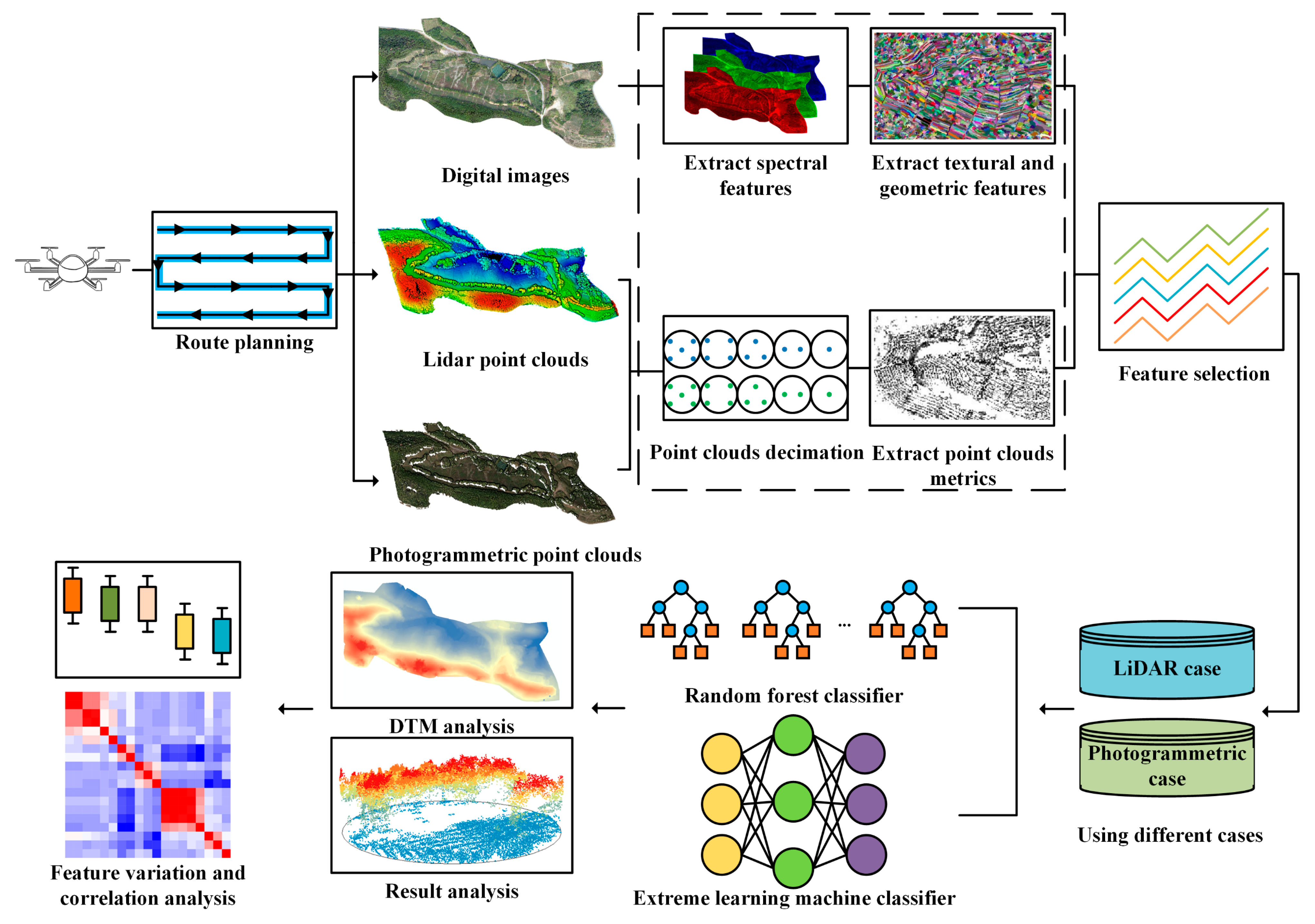
2. Materials and Methods

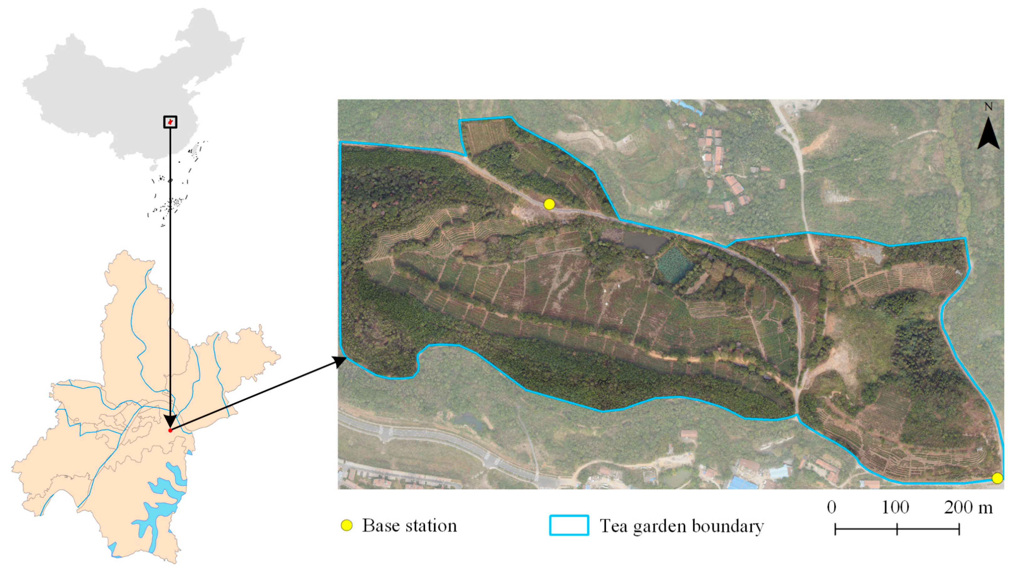
2.1. Study Area

This study was conducted in Huashan Tea Garden, Wuhan City, China (114°30′36.11″E, 30°33′50.39″N) (Figure 2). The study area has a subtropical monsoon climate with an annual temperature of 15.8–17.5 °C and an annual precipitation of 1150–1450 mm. The study area was 35.25 ha in size, with an elevation ranging from 8.1 to 83.51 m above sea level, high in the southwest and low in the northeast. In the Huashan Tea Garden, the local specialty green tea “Huashan Tender Bud” is produced, and the garden is also an ecological park where the public has the opportunity to observe and experience tea plucking.

2.2. UAV Data and Processing

2.2.1. LiDAR Data

LiDAR data were collected on 1 October 2019 by a Velodyne LiDAR VLP-16 Puck sensor (Velodyne LiDAR Inc., San Jose, CA, USA), which was mounted on a DJI M600 UAV (DJI, Shenzhen, China). The sensor was small (103 × 72 mm) and weighed 830 g. With 16 scanning channels and a wavelength of 903 nm, the sensor had a measuring range of 100 m and a range accuracy of 3 cm. We performed three flights in the study area with an altitude of approximately 60 m above ground level and a flight speed of 5 m/s. The average point density was 25.44 pts/m².

Before obtaining forest structural information from the point clouds, some preprocessing was required to create a digital terrain model (DTM) of the study area. First, the point clouds were classified as ground or nonground points using an improved progressive triangulated irregular network (TIN) densification filtering algorithm [35]. Second, a 0.1 m DTM was generated using ground returns and standard preprocessing routines [36]. Additionally, a digital surface model (DSM) with a spatial resolution of 0.1 m was generated. Then, a 0.1 m canopy height model (CHM) was generated by subtracting the DTM from the DSM. LiDAR data processing was performed using POSPac UAV 8.1 software (Applanix, Richmond Hill, ON, Canada) and LiDAR360 software (GreenValley, Beijing, China).

2.2.2. Photogrammetric Data

Digital imagery was acquired using an EOS 5D camera mounted on a DJI M600 UAV on 1 October 2019. We performed one flight at an altitude of 300 m above ground level. The imagery was 3-band (red, green, and blue) with a spatial resolution of 0.1 m. Image-based point clouds were generated using image-matching algorithms [37]. In this study, Pix4Dmapper software (Pix4D, Prilly, Switzerland) was used to generate photogrammetric point clouds. This software uses static images to generate point clouds. The point clouds were generated based on automatic tie points (ATPs), which are 3D points that are automatically detected and matched in the images and used to compute 3D positions. The Pix4D-derived point clouds record the horizontal, vertical, and color information of each point. The photogrammetric point density was 22.27 pts/m². The data processing was consistent with the LiDAR point clouds, resulting in the formation of the DTM, DSM, and CHM, all with spatial resolutions of 0.1 m.

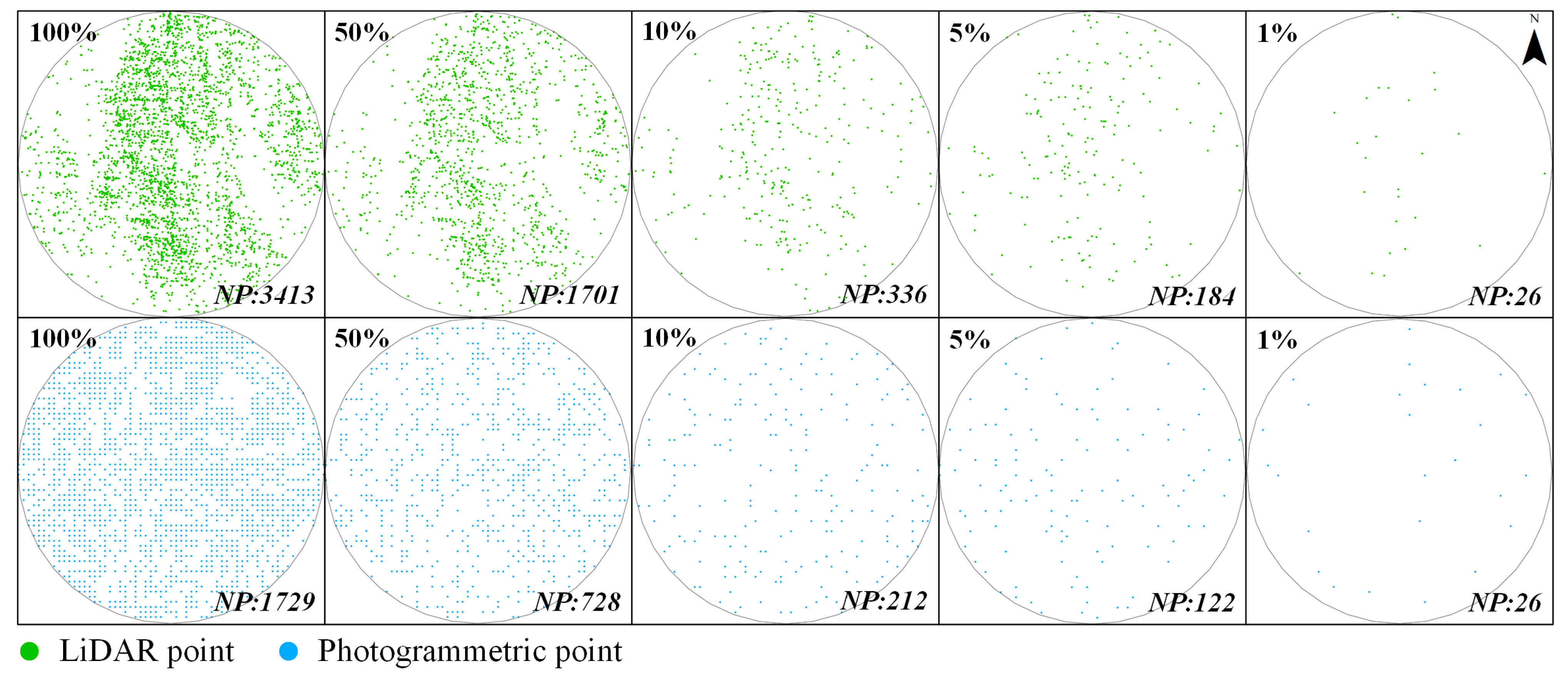
2.3. Point Cloud Data Decimation and Feature Extraction

LiDAR and photogrammetric point clouds were decimated from the original point densities (25.44 and 22.27 pts/m²) to lower densities of 50% (12.71 and 9.72 pts/m²), 10% (2.55 and 2.46 pts/m²), 5% (1.27 and 1.65 pts/m²), and 1% (0.25 and 0.36 pts/m²) of the original densities (Figure 3) using the “Decimate LAS File(s) by percent” utility developed at the Boise Center Aerospace Laboratory, Boise, Idaho (BCAL LiDAR Tools, 2013) [27]. We selected this point cloud reduction approach over other approaches, such as the given number of points or points spacing, for two reasons. Firstly, this approach ensured consistency between the two types of point clouds; secondly, it maintained a similar spatial distribution in the decimated point clouds to in the original point clouds.

We extracted 34 commonly used LiDAR/photogrammetric metrics (i.e., 21 for height, 3 for canopy volume, and 10 for density) using LiDAR360 software (GreenValley, Beijing, China), based on previous studies related to crops and forests [38,39,40]. The digital images were segmented into individual objects to obtain the corresponding feature parameters for the object-based image analysis. In addition to containing spectral information, object-based digital images also provide internal spatial information such as geometric and textural features [41]. We extracted 10 optical features using eCognition Developer 9.0.1 (Trimble, Sunnyvale, CO, USA) software.

Table 1. List of metrics derived from the UAV-LiDAR/photogrammetric point clouds.

LiDAR Metrics		Implication
Height metrics	HMean	Mean of heights
	HSD, HVAR	Standard deviation of heights and variance of heights
	HAAD	Average absolute deviation of heights
	HIQ	Interquartile distance of percentile height, H75th–H25th
	Percentile heights (H1, H5, H10, H20, H25, H30, H40, H50, H60, H70, H75, H80, H90, H95, and H99)	Height percentiles. Point clouds are sorted according to the elevation. Fifteen height percentile metrics ranging from 1% to 99% height
	Canopy height model value	Value of CHM: $\mathrm{CHM}=\mathrm{DSM}-\mathrm{DTM}$
Canopy volume metrics	CC0.2m	Canopy cover above 0.2 m
	Gap	Canopy volume-related metric
	Leaf area index	Dimensionless quantity that characterizes plant canopies
Density metrics	Canopy return density (D0, D1, D2, D3, D4, D5, D6, D7, D8, and D9)	The proportion of points above the quantiles to the total number of points

and

Table 2. List of features derived from the UAV digital imagery.

Feature	Implication
Spectral mean values (RGB)	The average spectral luminance of all pixels in a wavelength band within an image object
Brightness	Reflects the total spectral luminance difference among image objects
Length/width	Represented by a minimal outsourcing rectangle
Shape index	Used to reflect the smoothness of image object boundaries
Textural feature	Entropy, contrast, homogeneity, and correlation calculated through the gray-level co-occurrence matrix (GLCM) with a distance of 1 [42]. The GLCM is a matrix used to count the correlations between the gray levels of two pixels at a given spacing and orientation in an image

show the point cloud metrics and digital imagery features used in this study, respectively.

2.4. Classification Algorithms and Feature Selection

2.4.1. Classification Algorithms

The extreme learning machine and random forest algorithms were used to classify tea plantations and surrounding land covers into four classes (tea, building, water, vegetation (non-tea)) using UAV-derived data (including imagery and point cloud data with different densities). The extreme learning machine (ELM) is an algorithm proposed by Huang et al. [43,44] with the ability to operate quickly and with a good generalization performance that can be applied to regression and classification problems. The ELM is a feedforward neural network with a simple three-layer structure: input layer, hidden layer, and output layer. If we let $n$ be the number of input layer nodes, $r$ be the number of hidden layer nodes, and $c$ be the number of output layer nodes, the output ($O_j$) of $N$ training samples can be calculated using ELM with the following equation [45]:

$$O_j={\displaystyle \sum }_{i=1}^r{\beta }_i\ast g\left(w_i\ast x_j+b_i\right), j=1, 2,\dots ,N$$

(1)

where $x_j$ is the jth training sample, $w_i$ is the weight vector connecting the $i$th hidden node to the input nodes, ${\beta }_i$ is the weight vector connecting the $i$th hidden node to the output nodes, $g\left(x\right)$ is an activation function, and $b_i$ is the threshold of the $i$th hidden node. Previous research has demonstrated that we just need to set the number of hidden nodes and not change the input weights or the threshold of the hidden layer [46]. This results in only one optimal solution. In this study, the number of hidden nodes was set to 300, and the sigmoid function was used as the activation function.

The random forest (RF) algorithm was chosen in this study because it has been successfully applied in previous studies on the classification of tree species [47] and crops [48].

2.4.2. Feature Selection

An RF-based recursive feature elimination (RFE) algorithm was used to select the features from optical imagery and point clouds with different densities. This algorithm comprises a recursive process and compares the cross-validated classification performance of feature data sets as the number of features is reduced [49,50]. The key of RFE is to iteratively build the training model; then, the best feature data set is retained based on the out-of-bag error [49]. We implemented the RFE algorithm using the Python 3.6 programming language and the RFECV function from the scikit-learn 0.23.2 library. Two hyper-parameters are crucial in the RFECV function: step and cv. The step parameter controls the number of features to be removed at each iteration, and the cv parameter determines the number of folds used for cross-validation. In this study, both were set to the default values (step = 1 and cv = 3).

To systematically assess the performance of LiDAR and photogrammetric point clouds with different densities when mapping the plucking area of tea plantations, two cases of tea plucking area identification were designed based on different combinations of UAV remotely sensed data: the LiDAR case, which consisted of a combination of LiDAR metrics and optical imagery features, and the photogrammetric case, which consisted of a combination of photogrammetric metrics and optical imagery features. Figure 4 shows a schematic graph of the point cloud performance comparison using two cases.

2.5. Accuracy Assessment

The produced DTMs and thematic maps both needed to be assessed. We randomly selected 100 points in the original LiDAR point cloud from the bare ground areas as a validation sample set. The Z-values of the sample points were considered to represent the true elevation values of the ground and were used as an independent data set to assess the vertical error in the DTMs. The mean absolute error (MAE) and root mean square error (RMSE) were calculated to evaluate the global accuracy of the DTMs.

A classification confusion matrix, including the overall classification accuracy (OA) and Kappa coefficient, was used to evaluate the classification accuracy [51]. A set of 5076 samples was randomly selected and collected based on the field survey results and optical images after multiresolution segmentation. The samples were divided into a training set, and a validation set with a ratio of 7:3 to evaluate the classification accuracy.

Additionally, an area-based accuracy assessment method was applied to tea (refers to the tea plucking area) and non-tea areas (i.e., building, water, and vegetation areas) to measure the level of similarity between the classification results and reference data (maps from visual interpretation) by three indicators (

Table 3. Area-based accuracy assessment equations.

Indicator	Equations
ABUA	(|C∩R|)/(|C|)
ABPA	(|C∩R|)/(|R|)
ABOA	$\left(\right|\mathrm{C}{\displaystyle \cap }$$\mathrm{R}\left|\right)/\left(\right|\mathrm{C}{\displaystyle \cup }$R|)

C is the area of the classification results, and R is the area of the visually interpreted reference results.

), namely, the area-based user’s accuracy (ABUA), the area-based producer’s accuracy (ABPA), and the area-based overall accuracy (ABOA) [52]. In particular, ABOA was defined as the ratio between the correctly classified area (both classes) and the total area of observation. The visual interpretation results from the digital imagery with a spatial resolution of 0.1 m were considered to be true cover types [53]. We randomly generated 10 circular areas with a 30 m radius in the study area to calculate the area-based accuracy according to the method developed by Whiteside et al. [54] (Figure 5).

3. Results

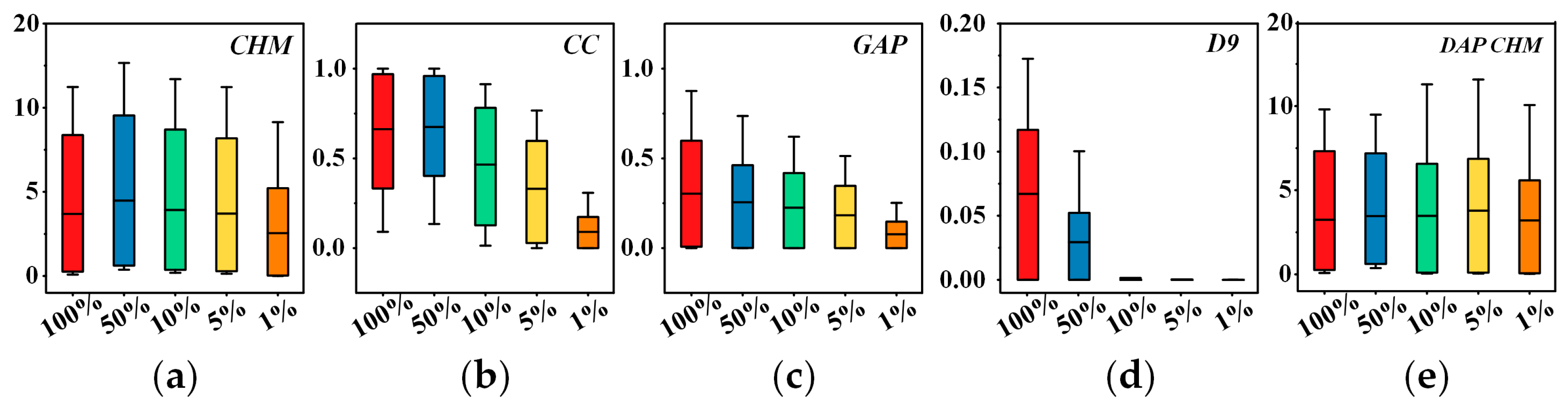
3.1. Point Density Effect on the DTM

The densities of the ground returns of LiDAR point clouds ranged from 0.08 to 0.84 points/m², and the densities of the ground returns of photogrammetric point clouds ranged from 0.17 to 1.16 points/m² (

Table 4. Summary of the point cloud return densities.

Type		Density of All Returns (pts/m2)	Density of Ground Returns (pts/m2)
LiDAR 1	100	25.44	0.84
	50	12.71	0.65
	10	2.55	0.35
	5	1.27	0.24
	1	0.25	0.08
Photogrammetric 2	100	22.27	1.16
	50	9.72	1.13
	10	2.46	0.71
	5	1.65	0.55
	1	0.36	0.17

¹ Percentage of original LiDAR data. ² Percentage of original photogrammetric data.

).

For DTMs generated from point clouds with different densities, the MAEs for LiDAR and photogrammetric data ranged from 0.038 to 0.735 m and from 0.23 to 0.274 m, respectively (

Table 5. Statistics of errors for DTMs of the tea plantation with different point densities.

Type		Density of Ground Returns (pts/m2)	MAE (m)	RMSE (m)
LiDAR 1	100	0.84	0.038	0.060
	50	0.65	0.051	0.072
	10	0.35	0.059	0.087
	5	0.24	0.337	1.884
	1	0.08	0.735	2.253
Photogrammetric 2	100	1.16	0.23	0.256
	50	1.13	0.241	0.266
	10	0.71	0.244	0.268
	5	0.55	0.236	0.261
	1	0.17	0.274	0.477

1 m DTMs were interpolated by the triangulated irregular network (TIN) interpolation algorithm. ¹ Percentage of original LiDAR data. ² Percentage of original photogrammetric data.

). The RMSEs ranged from 0.060 to 2.253 m for LiDAR data and from 0.256 to 0.477 m for photogrammetric data. Overall, the DTM error increased significantly when the original LiDAR data were decimated to 5% and 1%, while the error of the photogrammetric data varied slightly when the point densities were reduced.

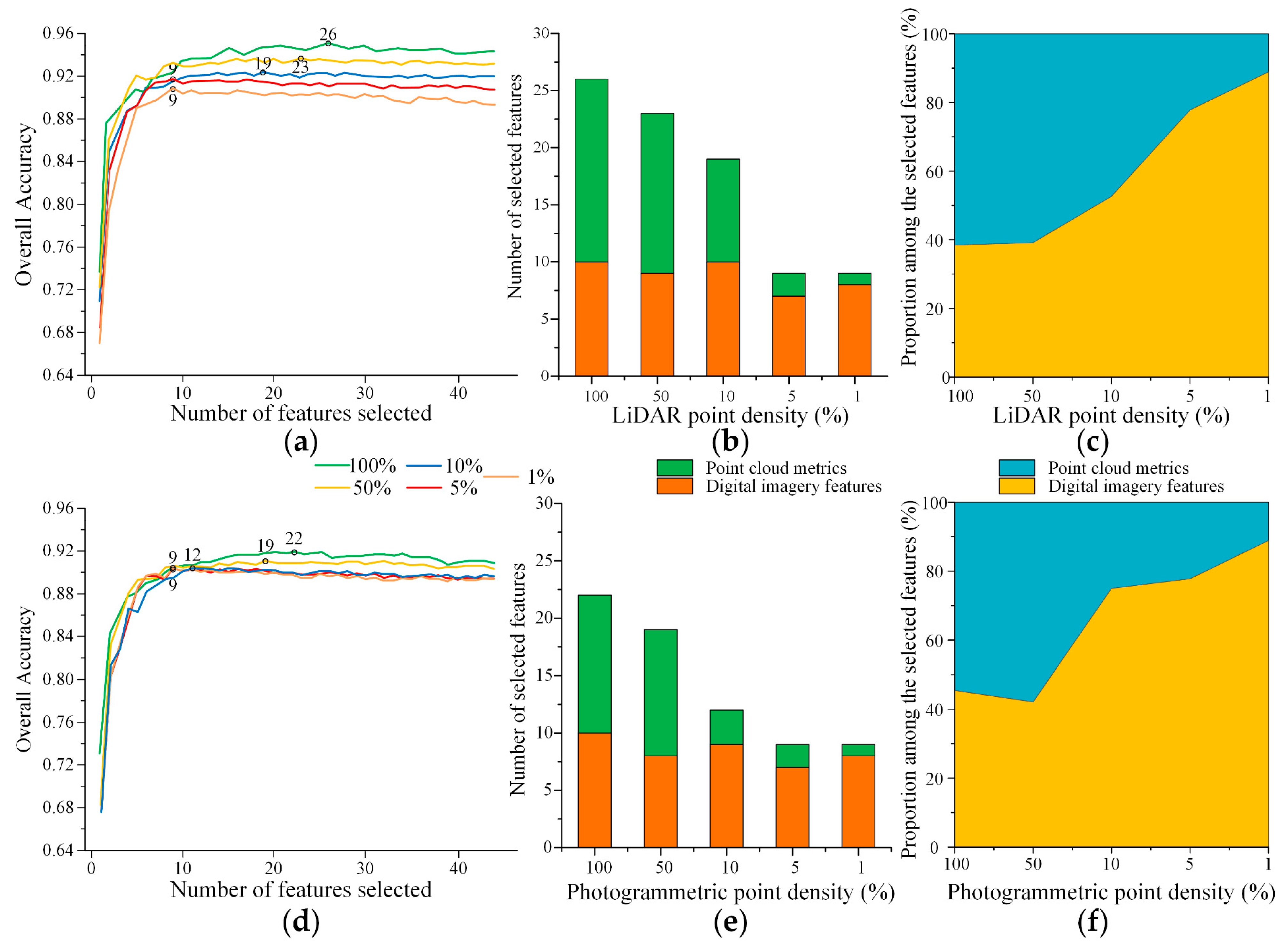
3.2. Point Density Effect on Feature Selection

Point clouds can provide a wealth of horizontal and vertical information about plants [24]. Reducing the point density dilutes the vertical complexity, resulting in a reduction in the importance of some point cloud metrics [27]. Figure 6 shows the feature selection results and performances with different point densities. The numbers (Figure 6b,e) and percentages (Figure 6c,f) of point clouds and image features are also presented.

Table 6. List of selected features for the LiDAR case with different LiDAR point densities.

LiDAR 1	Point Density (point/m2)	Number of Selected Features	Description of Selected Features
100	25.44	26 (16)	Red band, green band, blue band, brightness, length/width, shape index, entropy, contrast, homogeneity, correlation, D0, D9, LAI (leaf area index), Gap, CC0.2m, H10, H80, H90, H95, H99, HVAR, HIQ, HAAD, HMean, HSD, and CHM
50	12.71	23 (14)	Red band, green band, blue band, brightness, length/width, shape index, entropy, contrast, homogeneity, D8, LAI, Gap, CC0.2m, H20, H25, H40, H50, H60, H70, H75, HVAR, HMean, and CHM
10	2.55	19 (9)	Red band, green band, blue band, brightness, length/width, shape index, entropy, contrast, homogeneity, correlation, D1, D3, LAI, Gap, CC0.2m, H30, H40, HVAR, and CHM
5	1.27	9 (2)	Red band, green band, blue band, brightness, length/width, shape index, entropy, Gap, and CHM
1	0.25	9 (1)	Red band, green band, blue band, brightness, length/width, shape index, entropy, contrast, and CHM

The value in parentheses beside the number of selected features indicates the number of LiDAR features. ¹ Percentage of original LiDAR data.

and

Table 7. List of selected features for the photogrammetric case with different photogrammetric point densities.

Photogrammetric 1	Point Density (point/m2)	Number of Selected Features	Description of Selected Features
100	22.27	22 (12)	Red band, green band, blue band, brightness, length/width, shape index, entropy, contrast, homogeneity, correlation, Gap, CC0.2m, H10, H80, H90, H95, H99, HIQ, HAAD, HMean, HSD, and CHM
50	9.72	19 (11)	Red band, green band, blue band, brightness, length/width, shape index, entropy, contrast, LAI, Gap, CC0.2m, H20, H25, H50, H60, H70, HVAR, HMean, and CHM
10	2.46	12 (3)	Red band, green band, blue band, brightness, length/width, shape index, entropy, contrast, homogeneity, Gap, CC0.2m, and CHM
5	1.65	9 (2)	Red band, green band, blue band, brightness, length/width, shape index, entropy, Gap, and CHM
1	0.36	9 (1)	Red band, green band, blue band, brightness, length/width, shape index, entropy, contrast, and CHM

The value in parentheses beside the number of selected features indicates the number of photogrammetric features. ¹ Percentage of original photogrammetric data.

summarize the selected features from the digital imagery and point cloud data with different densities.

With the decimation of the point cloud density, the number of selected features decreased. The optimal numbers of features were 26, 23, 19, 9, and 9 for the LiDAR case and 22, 19, 12, 9, and 9 for the photogrammetric case. Regarding the LiDAR case, LiDAR metrics describing the top morphological characteristics of the canopy, such as H70 and H95, gradually disappeared as the point cloud density decimated. Additionally, HVAR and HSD, which describe the overall distribution characteristics of the canopy, persisted even when the point density was reduced to 10% (2.55 pts/m²) of the original point density. CHM and GAP were also always considered important. For the photogrammetric case, the point cloud features showed a precipitous reduction as the density reduced to 10% of the original point density, but CHM was always regarded as significant.

3.3. Point Density Effect on Classification Accuracy

3.3.1. Algorithm Accuracy Assessment

The classification accuracy levels of the LiDAR and photogrammetric cases performed with the RF and ELM algorithms are presented in

Table 8. Summary of classification accuracy levels using the RF and ELM based on the validation sample set.

Data	Percentage of Point Densities	RF	ELM
		OA (Kappa)	OA (Kappa)
LiDAR	100	94.39% (0.91)	93.44% (0.91)
	50	93.80% (0.90)	92.98% (0.89)
	10	93.01% (0.88)	92.27% (0.87)
	5	91.93% (0.86)	90.89% (0.85)
	1	90.65% (0.85)	89.78% (0.85)
Photogrammetric	100	91.58% (0.86)	90.07% (0.86)
	50	91.04% (0.85)	89.74% (0.84)
	10	90.55% (0.84)	89.25% (0.83)
	5	90.64% (0.84)	88.57% (0.83)
	1	90.55% (0.84)	88.32% (0.83)

. The overall classification accuracy using optical images was 87.65%.

Overall, the classification accuracy levels reduced as the point density was decimated and the variation was within 4%. The RF-based and ELM-based classifications performed similarly regarding the overall classification accuracy, and the RF produced a higher level of accuracy than the ELM. The highest level of accuracy (94.39%) was achieved by the LiDAR case with the 100% density point cloud using the RF algorithm.

For the LiDAR case, the RF algorithm produced a high level of accuracy (OA: 93.01–94.39% and kappa: 0.88–0.91) when the point density was 100%, 50%, and 10% that of the original data, and a similar trend existed when using the ELM algorithm (OA: 92.27–93.44% and kappa: 0.87–0.91). However, when the LiDAR point density decreased to 5%, there was a significant reduction in the OA (>1%) and kappa (>0.2) for both the RF and ELM. For photogrammetric case, the OA and kappa reduced slightly as the point density decimated (OA: 90.55–91.58% and kappa: 0.84–0.86 for RF; OA: 88.32–90.07% and kappa: 0.83–0.86 for ELM).

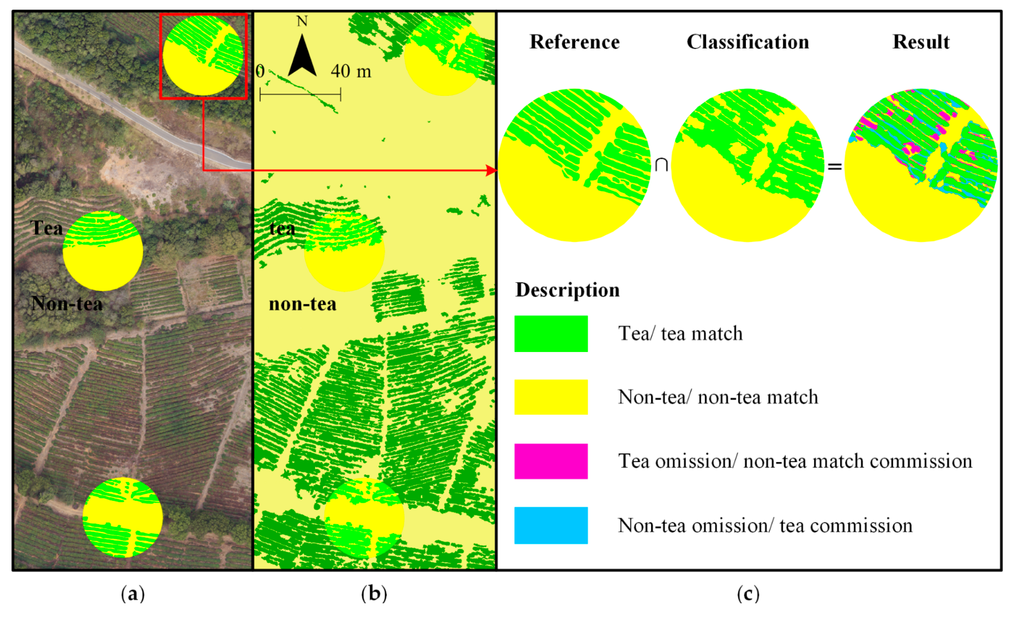
3.3.2. Area-Based Accuracy Assessment

The main strength of this method is its intuitive and visual evaluation of the classification result, especially for tea plucking areas.

Table 9. Summary of the area-based descriptive statistics as percentages (%) using the RF algorithm. ABUA: area-based user’s accuracy; ABPA: area-based producer’s accuracy; ABOA: area-based overall accuracy.

Density 1	Class	LiDAR			Photogrammetric
		ABUA	ABPA	ABOA	ABUA	ABPA	ABOA
100	tea	78.46	85.07	87.63	76.42	74.34	84.32
	non-tea	92.57	88.81		87.91	89.05
50	tea	76.56	86.22	87.01	74.41	80.12	83.58
	non-tea	92.99	87.36		90.15	86.85
10	tea	75.86	79.87	85.49	73.84	73.60	83.04
	non-tea	90.14	87.87		87.42	87.55
5	tea	72.79	72.61	82.64	72.52	71.86	82.11
	non-tea	87.29	87.40		86.59	86.96
1	tea	72.05	71.04	81.47	71.56	70.79	81.57
	non-tea	86.41	85.75		86.25	86.69

¹ Percentage of original point cloud data.

and

Table 10. Summary of the area-based descriptive statistics as percentages (%) using the ELM algorithm. ABUA: area-based user’s accuracy; ABPA: area-based producer’s accuracy; ABOA: area-based overall accuracy.

Density 1	Class	LiDAR			Photogrammetric
		ABUA	ABPA	ABOA	ABUA	ABPA	ABOA
100	tea	76.54	82.92	86.64	76.93	74.83	84.54
	non-tea	92.61	88.42		88.02	89.17
50	tea	74.74	84.24	86.43	72.87	78.47	83.04
	non-tea	93.12	89.74		88.47	85.23
10	tea	75.83	79.46	85.42	73.74	73.43	83.12
	non-tea	90.11	90.55		87.61	87.75
5	tea	72.98	72.85	82.59	72.86	72.19	82.48
	non-tea	87.17	87.24		86.98	87.36
1	tea	72.28	71.20	81.58	70.98	70.21	81.28
	non-tea	86.02	86.53		87.11	86.53

¹ Percentage of original point cloud data.

show the area-based accuracy assessment for the classification results of both the LiDAR and photogrammetric cases using the RF and ELM algorithms.

For the LiDAR case, the ABOA values of RF and ELM were high (85.49–87.63% and 85.42–86.64%, respectively) when the point densities were 100%, 50%, and 10% of the original data. However, when the point densities decreased to 5% and 1% of those in the original data, there was a significant reduction in the ABOA (with 3–5% accuracy loss). Regarding the photogrammetric case, the ABOA reduced slightly as the point density was decimated, ranging from 84.32% to 81.57% for the RF and from 84.54% to 81.28% for the ELM. The accuracy variation among densities was not significant, which is consistent with the results from Section 3.3.1. In addition, the ABPA and ABUA values of tea were lower than those of non-tea.

3.4. Cost–Benefit Comparison

The inferred time and economic costs required to map the plucking area of a 100 ha tea garden four times (such as monitoring changes over the four seasons) are listed in

Table 11. Time and economic costs required for the LiDAR case and photogrammetric case used for mapping the plucking area of a 100 ha tea garden four times.

Component	Detailed Costs
	Photogrammetric Case					LiDAR Case
Flight height (m)	60	90	120	200	300	60	90	120	200	300
Point cloud density (pts/m2)	22.27	9.72	2.46	1.65	0.36	25.44	12.71	2.55	1.27	0.25
Scanning width (m)	100	150	200	334	500	100	150	200	334	500
Time consumed (hour)	12.80	8.53	6.40	3.83	2.56	44.80	29.86	22.40	13.41	8.96
Cost (USD)	2560	1706	1280	766	512	44,800	29,860	22,400	13,410	8960
Cost (USD per ha)	25.60	17.06	12.80	7.66	5.12	448	299	224	134	90

for the photogrammetric case and LiDAR case at different flight heights. Each flight had the same lateral overlap ratio (50%). The costs were estimated in USD/km² based on the average price of the rental service provided for mapping and surveying fields in China: ~USD 1000 per hour for the LiDAR case and ~USD 200 per hour for the photogrammetric case. With an increase in flight height from 60 to 300 m, the time required to map a 100 ha tea garden four times reduced from 12.80 to 2.56 h using the photogrammetric case and from 44.80 to 8.96 h using the LiDAR case. Furthermore, the LiDAR case required more time and greater economic cost than the photogrammetric case (time consumed: 44.80 vs. 12.80 h and cost: USD 448 vs. 25.60 per ha at a flight height of 60 m in our study). The time and economic costs of the LiDAR method for mapping a 100 ha tea garden were four and 17 times greater than those required for the photogrammetric method overall.

4. Discussion

This is the first study to focus on examining the effects of UAV-LiDAR and photogrammetric point density on tea plucking area identification. The optimal point density of LiDAR data in combination with optical imagery for tea plucking area identification were determined for the first time. Our study has significant and practical meaning for the regular monitoring and precise management of tea plantations. The results of this study could help other scrub researchers and managers to choose the appropriate UAV equipment and flight parameters according to their needs. Additionally, our results reveal that the height metrics are the most important metrics, confirming the applicability of vertical information in classifying tea plants from surrounding vegetation.

4.1. Performance of LiDAR and Photogrammetric Data

In this study, we used a DJI M600 multi-rotor UAV, which provided a suitable platform for the LiDAR sensor by maintaining stability during the flight mission [55]. Then, a lightweight LiDAR sensor (Velodyne Puck VLP-16) and a digital camera (EOS 5D) were mounted on the UAV to collect point clouds and images.

The results demonstrate that UAV point cloud data are suitable for mapping tea plucking area at a finer scale. When different densities of LiDAR point clouds (100%, 50%, 10%, 5%, and 1% of the original point clouds) were used, the RMSEs of the DTM were 0.060, 0.072, 0.087, 1.884, and 2.253 m, respectively. For photogrammetric point clouds, the RMSEs of DTM were 0.256, 0.266, 0.268, 0.261, and 0.477 m. This indicated that as the point cloud density decreased, there was a significant increase in the error of the DTMs generated by LiDAR data, while the accuracy levels of the DTMs generated from photogrammetric data did not change much. One reason for this is that when the photogrammetric point cloud was generated by the image matching algorithm, more ground points were extracted and maintained to ensure the matching process was completed [56,57]. As a consequence, there was no significant reduction in the accuracy of the DTM with a high proportion of ground points in the photogrammetric point clouds. However, the LiDAR data were capable of achieving a higher level of accuracy (root mean square error < 10 cm; mean absolute error < 10 cm) in comparison with the photogrammetry point clouds, indicating that LiDAR data may be more suitable for producing a precise DTM in a tea garden.

The advantage of the LiDAR case was that it was able to obtain accurate point clouds with sufficient information about the vertical structures, resulting in highly accurate predicted metrics and classification results (OA = 94.39% and ABOA = 87.63% for RF; OA = 93.44% and ABOA = 86.64% for ELM). However, the photogrammetric case was shown to be advantageous in terms of time and economic costs. It is possible for a working team of three people to map a 100 ha tea garden within 3.2 h using the photogrammetric case at a flight altitude of 60 m, while this team would spend 11.2 h if the LiDAR case was used at the same flight altitude. Additionally, compared with the LiDAR case, the financial benefits afforded by the photogrammetric case are obvious. With a flight height of 60 m, the cost for mapping the plucking area of a 100 ha tea garden four times would be USD 42,200 cheaper for the photogrammetric case than for the LiDAR case (Table 11); however, with the development of LiDAR scanners, the cost of the LiDAR case will be lower. For instance, the DJI Livox Mid40 laser scanner costs only USD 600, which could significantly improve the cost–benefit of the LiDAR case.

Overall, the use of photogrammetric point clouds for capturing upper canopy and terrain surface information was demonstrated to be competitive. However, several major limitations also exist. Firstly, photogrammetric point clouds have a low sensitivity to low intensity return signals [58], resulting in a large proportion of internal canopy information being missed in areas of dense canopy as shown in Figure 7. This might lead to biases in the generation of the point cloud metrics. Secondly, the photogrammetric case must set more flight lines than the LiDAR case at the same flight height due to the narrow field of view of an ordinary digital camera, while with increasing flight lines, more time is needed, and there may be more errors in the measurement. However, the photogrammetric case still can be used as an alternative to UAV LiDAR when LiDAR scanners are not available or funds are limited.

4.2. Point Cloud Density Effect on Mapping Tea Plucking Areas

Previous studies have demonstrated the effects of point density on the estimation of forest structural attributes [27]. It was found that the use of the optimized point density can maintain the mapping accuracy of urban tree species (Liu et al. [59]). This study enriched the research on LiDAR and photogrammetric point cloud density in tea plantation mapping. Our results suggest that reducing the point density may be a viable solution for minimizing data collection costs and overcoming operational efficiency challenges while maintaining the desired accuracy of tea plucking area identification.

In this study, we found that LiDAR data with point densities of 2.55–25.44 pts/m² can be used to carry out cost-effective point cloud data acquisition and processing for tea plantations over a large area to generate a DTM with a high level of accuracy and to identify tea plucking areas precisely. The LiDAR point density within this range had little effect on the DTM generation (Table 5) and classification accuracy (Table 8, Table 9 and Table 10). The contributions of LiDAR data persisted even when the point density was reduced to 10% (2.55 pts/m²) of the original point density as shown in Figure 6b. We found that at a point density of 10%, there were still nine LiDAR features selected. Figure 8 represents five typical features of reduced point cloud densities and indicates that with a decrease in point density, there are no significant differences in CHM values or digital aerial photogrammetry (DAP) CHM values, while CC, GAP, and D9 showed a significant decreasing tendency as the density drops to 10% (2.55 pts/m²). Overall, the carrying information of point cloud features was shown to be largely invariant to point density changes at moderate to high densities. In particular, density metrics were found to be more sensitive to changes in point density, which is consistent with previous studies [26,60]. Height metrics and canopy volume metrics were relatively unaffected until the point densities dropped below 2.55 pts/ m². This explains why the classification accuracy changed slightly when the point density decreased from 100% to 10%. These findings are consistent with those of Cățeanu and Ciubotaru [61], who found that the reduction of LiDAR data to a certain extent did not affect the DTM or classification accuracy. Therefore, LiDAR data could be reduced without significantly impacting the accuracy of tea plantation mapping.

Regarding photogrammetric point clouds, Figure 7 shows that the vertical information in photogrammetric data was less than that in the LiDAR data. When the point density decreased from 100% to 10%, only three photogrammetric features remained (Table 7), which demonstrates that the decimation of point clouds also reduced the carrying information in photogrammetric point clouds. This explains why the accuracy of the photogrammetric case was lower than that of the LiDAR case.

To explore the specific role of each feature and to provide candidate features for subsequent studies, we proposed a hierarchical clustering-correlation method. We calculated the distances and hierarchical relationships among the features selected by the LiDAR case with a point density of 10% (the most cost-effective LiDAR point density in this study) as shown in Figure 9. The 19 features could be clustered into nine major categories at the 15 height (distance) level. H40, H30, D3, D1, and HVAR belong to one category; the width and shape index belong to one category; the red band, brightness, green band, blue band, Gap, and GLCM correlation belong to one category; and the other six features (i.e., LAI, CHM, CC, GLCM contrast, GLCM homogeneity, and GLCM entropy) were in a category each. Each feature subset or group in the hierarchical cluster plot had specific contributions to tea plucking area identification. The results suggest that the LiDAR metrics and texture features derived from optical imagery are important for tea plucking area mapping, which is consistent with the results of Weinmann et al. [62] and Liu, Coops, Aven, and Pang [59]. The correlation matrix heatmap shows the magnitude of Pearson’s correlation coefficient between two features and extends the information ascertained in the hierarchical clustering analysis [63]. Features in the same category are strongly correlated with each other, while features in different categories usually have low levels of correlation. Therefore, we suggest that the selection of features with close clustering groups (e.g., H30, H40, D1, and D4) should be reduced and features from different categories should be selected to ensure the selected features contain abundant information for classification. This hierarchical clustering-correlation diagram of important features reveals candidate features for tea plantation identification and provides a feature selection scheme that could be used in subsequent studies to improve efficiency.

At present, the relatively high cost of UAV-LiDAR systems is a major obstacle to their use in forest and agriculture applications [64,65]. Flight height was found to be the major factor influencing the point cloud density in the LiDAR and photogrammetric cases [66]. A flight height lower than 120 m (point density not less than 2.55 pts/m²) is suggested for the LiDAR case when used in tea plucking area identification. If the flight height is set to 120 m (an assumption) instead of 60 m using the same LiDAR scanner applied in this study, the method will be cost-effective (USD 12.80 cheaper per ha) while maintaining the mapping accuracy to the extent possible (only ~1% accuracy loss). The detection range of the LiDAR sensor needs to be considered when increasing the flight altitude. Currently, plenty of LiDAR sensors have long detection range greater than 120 m such as RIEGL miniVUX-1UAV (330 m) and Alpha Prime VLS-128 (200 m). Moreover, we also need to note that although the LiDAR sensor may theoretically generate a high-enough point density at increased altitudes, the number and accuracy of returns may be nonlinearly affected with increasing altitude, and the flight altitude should be adjusted appropriately based on the actual situation.

5. Conclusions

This study evaluated the performance of LiDAR and photogrammetric point cloud data with different densities in mapping the tea plucking area in the Huashan Tea Garden in China by using ELM and RF algorithms. We focused on screening significant features in LiDAR and photogrammetric cases with different point densities and establishing the linkages between point densities and variations in the DTM and classification accuracy. The LiDAR point cloud density was found to have a significant influence on the DTM and classification accuracy, while the photogrammetric point cloud density had a limited effect on the DTM and classification accuracy. However, the LiDAR point density had little effect on the feature selection and the accuracy levels of the DTM and classification when the density ranged from 100% (25.44 pts/m²) to 10% (2.55 pts/m²) of the original point density. LiDAR case performed best for tea plucking area identification, achieving an accuracy of 94.39% using the RF algorithm (ABOA = 87.63%) and 93.44% using the ELM algorithm (ABOA = 86.64%). Important features for tea plucking area identification were explored by a novel hierarchical clustering-correlation method: CHM and Gap were identified as the most important features from Lidar and photogrammetric cases with different densities.

This study demonstrates that reducing the point cloud density used in tea plucking area mapping is a feasible solution to (1) conduct mapping more efficiently, (2) reduce the cost of data acquisition, and (3) ensure accuracy as much as possible. The analysis of photogrammetric point clouds generated from UAV imagery demonstrates their potential for mapping the plucking area of tea plantations and shows that the density of the photogrammetric point has a low impact on accuracy and can, therefore, improve the operational efficiency. It can be used as an alternative to LiDAR point clouds in situations where equipment limitations exist.

References

1. Wang, B.; Li, J.; Jin, X.; Xiao, H. Mapping tea plantations from multi-seasonal Landsat-8 OLI imageries using a random forest classifier. J. Indian Soc. Remote Sens. 2019, 47, 1315–1329. [Google Scholar] [CrossRef]
2. Wambu, E.W.; Fu, H.Z.; Ho, Y.S. Characteristics and trends in global tea research: A Science Citation Index Expanded-based analysis. Int. J. Food Sci. Technol. 2017, 52, 644–651. [Google Scholar] [CrossRef]
3. Zhang, M.; Yonggen, C.; Dongmei, F.; Qing, Z.; Zhiqiang, P.; Kai, F.; Xiaochang, W. Temporal evolution of carbon storage in Chinese tea plantations from 1950 to 2010. Pedosphere 2017, 27, 121–128. [Google Scholar] [CrossRef]
4. Zhu, J.; Pan, Z.; Wang, H.; Huang, P.; Sun, J.; Qin, F.; Liu, Z. An improved multi-temporal and multi-feature tea plantation identification method using Sentinel-2 imagery. Sensors 2019, 19, 2087. [Google Scholar] [CrossRef] [Green Version]
5. Teke, M.; Deveci, H.S.; Haliloglu, O.; Gurbuz, S.Z.; Sakarya, U. A Short Survey of Hyperspectral Remote Sensing Applications in Agriculture; IEEE: New York, NY, USA, 2013; pp. 171–176. [Google Scholar]
6. Peña, J.M.; Gutiérrez, P.A.; Hervás-Martínez, C.; Six, J.; Plant, R.E.; López-Granados, F. Object-based image classification of summer crops with machine learning methods. Remote Sens. 2014, 6, 5019–5041. [Google Scholar] [CrossRef] [Green Version]
7. Csillik, O.; Kumar, P.; Mascaro, J.; O’Shea, T.; Asner, G.P. Monitoring tropical forest carbon stocks and emissions using Planet satellite data. Sci. Rep. 2019, 9, 17831. [Google Scholar] [CrossRef] [Green Version]
8. Lama, G.F.C.; Sadeghifar, T.; Azad, M.T.; Sihag, P.; Kisi, O. On the Indirect Estimation of Wind Wave Heights over the Southern Coasts of Caspian Sea: A Comparative Analysis. Water 2022, 14, 843. [Google Scholar] [CrossRef]
9. Sadeghifar, T.; Lama, G.; Sihag, P.; Bayram, A.; Kisi, O. Wave height predictions in complex sea flows through soft-computing models: Case study of Persian Gulf. Ocean Eng. 2022, 245, 110467. [Google Scholar] [CrossRef]
10. Imai, M.; Kurihara, J.; Kouyama, T.; Kuwahara, T.; Fujita, S.; Sakamoto, Y.; Sato, Y.; Saitoh, S.I.; Hirata, T.; Yamamoto, H.; et al. Radiometric calibration for a multispectral sensor onboard RISESAT microsatellite based on lunar observations. Sensors 2021, 21, 15. [Google Scholar] [CrossRef]
11. Maponya, M.G.; Van Niekerk, A.; Mashimbye, Z.E. Pre-harvest classification of crop types using a Sentinel-2 time-series and machine learning. Comput. Electron. Agric. 2020, 169, 105164. [Google Scholar] [CrossRef]
12. Rao, N.; Kapoor, M.; Sharma, N.; Venkateswarlu, K. Yield prediction and waterlogging assessment for tea plantation land using satellite image-based techniques. Int. J. Remote Sens. 2007, 28, 1561–1576. [Google Scholar]
13. Bian, M.; Skidmore, A.K.; Schlerf, M.; Wang, T.; Liu, Y.; Zeng, R.; Fei, T. Predicting foliar biochemistry of tea (Camellia sinensis) using reflectance spectra measured at powder, leaf and canopy levels. ISPRS J. Photogramm. Remote Sens. 2013, 78, 148–156. [Google Scholar] [CrossRef]
14. Chen, Y.-T.; Chen, S.-F. Localizing plucking points of tea leaves using deep convolutional neural networks. Comput. Electron. Agric. 2020, 171, 105298. [Google Scholar] [CrossRef]
15. Næsset, E.; Gobakken, T. Estimation of above- and below-ground biomass across regions of the boreal forest zone using airborne laser. Remote Sens. Environ. 2008, 112, 3079–3090. [Google Scholar] [CrossRef]
16. Puliti, S.; Ene, L.T.; Gobakken, T.; Næsset, E. Use of partial-coverage UAV data in sampling for large scale forest inventories. Remote Sens. Environ. 2017, 194, 115–126. [Google Scholar] [CrossRef]
17. Saponaro, M.; Agapiou, A.; Hadjimitsis, D.G.; Tarantino, E. Influence of Spatial Resolution for Vegetation Indices’ Extraction Using Visible Bands from Unmanned Aerial Vehicles’ Orthomosaics Datasets. Remote Sens. 2021, 13, 3238. [Google Scholar] [CrossRef]
18. Torresan, C.; Berton, A.; Carotenuto, F.; Di Gennaro, S.F.; Gioli, B.; Matese, A.; Miglietta, F.; Vagnoli, C.; Zaldei, A.; Wallace, L. Forestry applications of UAVs in Europe: A review. Int. J. Remote Sens. 2017, 38, 2427–2447. [Google Scholar] [CrossRef]
19. Lama, G.F.C.; Crimaldi, M.; Pasquino, V.; Padulano, R.; Chirico, G.B. Bulk Drag Predictions of Riparian Arundo donax Stands through UAV-Acquired Multispectral Images. Water 2021, 13, 1333. [Google Scholar] [CrossRef]
20. Song, K.; Brewer, A.; Ahmadian, S.; Shankar, A.; Detweiler, C.; Burgin, A.J. Using unmanned aerial vehicles to sample aquatic ecosystems. Limnol. Oceanogr. Meth. 2017, 15, 1021–1030. [Google Scholar] [CrossRef]
21. Jin, S.; Su, Y.; Song, S.; Xu, K.; Hu, T.; Yang, Q.; Wu, F.; Xu, G.; Ma, Q.; Guan, H. Non-destructive estimation of field maize biomass using terrestrial lidar: An evaluation from plot level to individual leaf level. Plant Methods 2020, 16, 69. [Google Scholar] [CrossRef]
22. Wang, D.; Wan, B.; Liu, J.; Su, Y.; Guo, Q.; Qiu, P.; Wu, X. Estimating aboveground biomass of the mangrove forests on northeast Hainan Island in China using an upscaling method from field plots, UAV-LiDAR data and Sentinel-2 imagery. Int. J. Appl. Earth Obs. Geoinf. 2020, 85, 101986. [Google Scholar] [CrossRef]
23. Scheller, J.H.; Mastepanov, M.; Christensen, T.R. Toward UAV-based methane emission mapping of Arctic terrestrial ecosystems. Sci. Total Environ. 2022, 819, 153161. [Google Scholar] [CrossRef] [PubMed]
24. Zhang, Q.; Wan, B.; Cao, Z.; Zhang, Q.; Wang, D. Exploring the potential of unmanned aerial vehicle (UAV) remote sensing for mapping plucking area of tea plantations. Forests 2021, 12, 1214. [Google Scholar] [CrossRef]
25. Næsset, E. Effects of different sensors, flying altitudes, and pulse repetition frequencies on forest canopy metrics and biophysical stand properties derived from small-footprint airborne laser data. Remote Sens. Environ. 2009, 113, 148–159. [Google Scholar] [CrossRef]
26. Jakubowski, M.K.; Guo, Q.; Kelly, M. Tradeoffs between lidar pulse density and forest measurement accuracy. Remote Sens. Environ. 2013, 130, 245–253. [Google Scholar] [CrossRef]
27. Singh, K.K.; Chen, G.; McCarter, J.B.; Meentemeyer, R.K. Effects of LiDAR point density and landscape context on estimates of urban forest biomass. ISPRS J. Photogramm. Remote Sens. 2015, 101, 310–322. [Google Scholar] [CrossRef] [Green Version]
28. Liu, K.; Shen, X.; Cao, L.; Wang, G.; Cao, F. Estimating forest structural attributes using UAV-LiDAR data in Ginkgo plantations. ISPRS J. Photogramm. Remote Sens. 2018, 146, 465–482. [Google Scholar] [CrossRef]
29. Dubayah, R.O.; Sheldon, S.; Clark, D.B.; Hofton, M.A.; Blair, J.B.; Hurtt, G.C.; Chazdon, R.L. Estimation of tropical forest height and biomass dynamics using lidar remote sensing at La Selva, Costa Rica. J. Geophys. Res. Biogeosci. 2010, 115, G00E09. [Google Scholar] [CrossRef]
30. Iglhaut, J.; Cabo, C.; Puliti, S.; Piermattei, L.; O’Connor, J.; Rosette, J. Structure from motion photogrammetry in forestry: A review. Curr. For. Rep. 2019, 5, 155–168. [Google Scholar] [CrossRef] [Green Version]
31. Filippelli, S.K.; Lefsky, M.A.; Rocca, M.E. Comparison and integration of lidar and photogrammetric point clouds for mapping pre-fire forest structure. Remote Sens. Environ. 2019, 224, 154–166. [Google Scholar] [CrossRef]
32. Lin, J.; Wang, M.; Ma, M.; Lin, Y. Aboveground tree biomass estimation of sparse subalpine coniferous forest with UAV oblique photography. Remote Sens. 2018, 10, 1849. [Google Scholar] [CrossRef] [Green Version]
33. Jurjević, L.; Liang, X.; Gašparović, M.; Balenović, I. Is field-measured tree height as reliable as believed–Part II, A comparison study of tree height estimates from conventional field measurement and low-cost close-range remote sensing in a deciduous forest. ISPRS J. Photogramm. Remote Sens. 2020, 169, 227–241. [Google Scholar] [CrossRef]
34. Cao, L.; Coops, N.C.; Sun, Y.; Ruan, H.; Wang, G.; Dai, J.; She, G. Estimating canopy structure and biomass in bamboo forests using airborne LiDAR data. ISPRS J. Photogramm. Remote Sens. 2019, 148, 114–129. [Google Scholar] [CrossRef]
35. Zhao, X.; Guo, Q.; Su, Y.; Xue, B. Improved progressive TIN densification filtering algorithm for airborne LiDAR data in forested areas. ISPRS J. Photogramm. Remote Sens. 2016, 117, 79–91. [Google Scholar] [CrossRef] [Green Version]
36. White, J.C.; Tompalski, P.; Coops, N.C.; Wulder, M.A. Comparison of airborne laser scanning and digital stereo imagery for characterizing forest canopy gaps in coastal temperate rainforests. Remote Sens. Environ. 2018, 208, 1–14. [Google Scholar] [CrossRef]
37. Leberl, F.; Irschara, A.; Pock, T.; Meixner, P.; Gruber, M.; Scholz, S.; Wiechert, A. Point clouds. Photogramm. Eng. Remote Sens. 2010, 76, 1123–1134. [Google Scholar] [CrossRef]
38. Kim, S.; McGaughey, R.J.; Andersen, H.-E.; Schreuder, G. Tree species differentiation using intensity data derived from leaf-on and leaf-off airborne laser scanner data. Remote Sens. Environ. 2009, 113, 1575–1586. [Google Scholar] [CrossRef]
39. Ritchie, C.J.; Evans, L.D.; Jacobs, D.; Everitt, H.J.; Weltz, A.M. Measuring Canopy Structure with an Airborne Laser Altimeter. Trans. ASAE 1993, 36, 1235–1238. [Google Scholar] [CrossRef]
40. Qiu, P.; Wang, D.; Zou, X.; Yang, X.; Xie, G.; Xu, S.; Zhong, Z. Finer resolution estimation and mapping of mangrove biomass using UAV LiDAR and worldview-2 data. Forests 2019, 10, 871. [Google Scholar] [CrossRef] [Green Version]
41. Haralick, R.M. Statistical and structural approaches to texture. Proc. IEEE 1979, 67, 786–804. [Google Scholar] [CrossRef]
42. Wang, D.; Wan, B.; Qiu, P.; Su, Y.; Guo, Q.; Wang, R.; Sun, F.; Wu, X. Evaluating the performance of Sentinel-2, Landsat 8 and Pléiades-1 in mapping mangrove extent and species. Remote Sens. 2018, 10, 1468. [Google Scholar] [CrossRef] [Green Version]
43. Huang, G.-B.; Zhu, Q.-Y.; Siew, C.-K. Extreme learning machine: Theory and applications. Neurocomputing 2006, 70, 489–501. [Google Scholar] [CrossRef]
44. Huang, G.-B.; Zhu, Q.-Y.; Siew, C.-K. Extreme learning machine: A new learning scheme of feedforward neural networks. In Proceedings of the 2004 IEEE International Joint Conference on Neural Networks (IEEE Cat. No. 04CH37541), Budapest, Hungary, 25–29 July 2004; pp. 985–990. [Google Scholar]
45. Han, M.; Liu, B. Ensemble of extreme learning machine for remote sensing image classification. Neurocomputing 2015, 149, 65–70. [Google Scholar] [CrossRef]
46. Moreno, R.; Corona, F.; Lendasse, A.; Graña, M.; Galvão, L.S. Extreme learning machines for soybean classification in remote sensing hyperspectral images. Neurocomputing 2014, 128, 207–216. [Google Scholar] [CrossRef]
47. Shang, X.; Chisholm, L.A. Classification of Australian native forest species using hyperspectral remote sensing and machine-learning classification algorithms. IEEE J. Sel. Top. Appl. Earth Observ. Remote Sens. 2013, 7, 2481–2489. [Google Scholar] [CrossRef]
48. Hariharan, S.; Mandal, D.; Tirodkar, S.; Kumar, V.; Bhattacharya, A.; Lopez-Sanchez, J.M. A novel phenology based feature subset selection technique using random forest for multitemporal PolSAR crop classification. IEEE J. Sel. Top. Appl. Earth Observ. Remote Sens. 2018, 11, 4244–4258. [Google Scholar] [CrossRef] [Green Version]
49. Pham, L.T.H.; Brabyn, L. Monitoring mangrove biomass change in Vietnam using SPOT images and an object-based approach combined with machine learning algorithms. ISPRS J. Photogramm. Remote Sens. 2017, 128, 86–97. [Google Scholar] [CrossRef]
50. Granitto, P.M.; Furlanello, C.; Biasioli, F.; Gasperi, F. Recursive feature elimination with random forest for PTR-MS analysis of agroindustrial products. Chemom. Intell. Lab. Syst. 2006, 83, 83–90. [Google Scholar] [CrossRef]
51. Ghosh, A.; Joshi, P.K. A comparison of selected classification algorithms for mapping bamboo patches in lower Gangetic plains using very high resolution WorldView 2 imagery. Int. J. Appl. Earth Obs. Geoinf. 2014, 26, 298–311. [Google Scholar] [CrossRef]
52. Kamal, M.; Phinn, S.; Johansen, K. Object-based approach for multi-scale mangrove composition mapping using multi-resolution image datasets. Remote Sens. 2015, 7, 4753–4783. [Google Scholar] [CrossRef] [Green Version]
53. Congalton, R.G. A review of assessing the accuracy of classifications of remotely sensed data. Remote Sens. Environ. 1991, 37, 35–46. [Google Scholar] [CrossRef]
54. Whiteside, T.; Boggs, G.; Maier, S. Area-based validity assessment of single- and multi-class object-based image analysis. In Proceedings of the 15th Australasian Remote Sensing and Photogrammetry Conference, Alice Springs, Australia, 13–17 September 2010. [Google Scholar]
55. Wallace, L.; Lucieer, A.; Watson, C.; Turner, D. Development of a UAV-LiDAR system with application to forest inventory. Remote Sens. 2012, 4, 1519–1543. [Google Scholar] [CrossRef] [Green Version]
56. Zhang, Z.; Gerke, M.; Vosselman, G.; Yang, M.Y. Filtering photogrammetric point clouds using standard LiDAR filters towards dtm generation. ISPRS Ann. Photogramm. Remote Sens. Spatial Inf. Sci. 2018, IV-2, 319–326. [Google Scholar] [CrossRef] [Green Version]
57. Barbasiewicz, A.; Widerski, T.; Daliga, K. The analysis of the accuracy of spatial models using photogrammetric software: Agisoft Photoscan and Pix4D. In Proceedings of the E3S Web of Conferences, Avignon, France, 4–5 June 2018; p. 00012. [Google Scholar]
58. Ma, Q.; Su, Y.; Guo, Q. Comparison of canopy cover estimations from airborne LiDAR, aerial imagery, and satellite imagery. IEEE J. Sel. Top. Appl. Earth Observ. Remote Sens. 2017, 10, 4225–4236. [Google Scholar] [CrossRef]
59. Liu, L.; Coops, N.C.; Aven, N.W.; Pang, Y. Mapping urban tree species using integrated airborne hyperspectral and LiDAR remote sensing data. Remote Sens. Environ. 2017, 200, 170–182. [Google Scholar] [CrossRef]
60. Næsset, E. Effects of different flying altitudes on biophysical stand properties estimated from canopy height and density measured with a small-footprint airborne scanning laser. Remote Sens. Environ. 2004, 91, 243–255. [Google Scholar] [CrossRef]
61. Cățeanu, M.; Ciubotaru, A. The effect of lidar sampling density on DTM accuracy for areas with heavy forest cover. Forests 2021, 12, 265. [Google Scholar] [CrossRef]
62. Weinmann, M.; Jutzi, B.; Hinz, S.; Mallet, C. Semantic point cloud interpretation based on optimal neighborhoods, relevant features and efficient classifiers. ISPRS J. Photogramm. Remote Sens. 2015, 105, 286–304. [Google Scholar] [CrossRef]
63. Kučerová, D.; Vivodová, Z.; Kollárová, K. Silicon alleviates the negative effects of arsenic in poplar callus in relation to its nutrient concentrations. Plant Cell Tissue Organ Cult. 2021, 145, 275–289. [Google Scholar] [CrossRef]
64. Mandlburger, G.; Pfennigbauer, M.; Schwarz, R.; Flöry, S.; Nussbaumer, L. Concept and performance evaluation of a novel UAV-borne topo-bathymetric LiDAR sensor. Remote Sens. 2020, 12, 986. [Google Scholar] [CrossRef] [Green Version]
65. Hu, T.; Sun, X.; Su, Y.; Guan, H.; Sun, Q.; Kelly, M.; Guo, Q. Development and performance evaluation of a very low-cost UAV-LiDAR system for forestry applications. Remote Sens. 2021, 13, 77. [Google Scholar] [CrossRef]
66. Jurjević, L.; Gašparović, M.; Liang, X.; Balenović, I. Assessment of close-range remote sensing methods for DTM estimation in a lowland deciduous Forest. Remote Sens. 2021, 13, 2063. [Google Scholar] [CrossRef]
Figure 1. An illustration of a UAV-LiDAR data collection scheme in the Huashan Tea Garden (the study area). The UAV flight height affects the point cloud density and acquisition efficiency. Each flight had the same lateral overlap ratio (50%), and the number of flight lines was determined by the flight height.
Remotesensing 14 01505 g001
Figure 2. Location of the study area (the Huashan Tea Garden) in Wuhan City, China.
Remotesensing 14 01505 g002
Figure 3. Illustration of percentage-based LiDAR and photogrammetric point cloud decimation. The radius was 5 m, and NP denotes the number of points.
Remotesensing 14 01505 g003
Figure 4. A schematic graph of the point cloud performance comparison with LiDAR and photogrammetric cases.
Remotesensing 14 01505 g004
Figure 5. Illustration of the tea and non-tea area-based accuracy assessment: (a) digital imagery with a spatial resolution of 0.1 m; (b) thematic map produced using the random forest algorithm; (c) the classes produced from the area intersection process.
Remotesensing 14 01505 g005
Figure 6. Variation in the overall accuracy with different numbers of features selected by the RF-based RFE algorithm and the details of the selected features for the LiDAR case (ac) and photogrammetric case (df).
Remotesensing 14 01505 g006
Figure 7. Illustration of percentage-based UAV point cloud data density reduction.
Remotesensing 14 01505 g007
Figure 8. Variations of the LiDAR and photogrammetric features with reduced point densities: (ad) LiDAR features; (e) photogrammetric features.
Remotesensing 14 01505 g008
Figure 9. Hierarchical cluster plot and correlation matrix heatmap of important features in the LiDAR case with a point density of 10%. The 10% point density was the most cost-effective LiDAR point density found in this study. The upper graph represents hierarchical construction and distance among features; the below graph portrays pairwise correlation between features.
Remotesensing 14 01505 g009