Robust Object Categorization and Scene Classification over Remote Sensing Images via Features Fusion and Fully Convolutional Network

Abstract

The latest visionary technologies have made an evident impact on remote sensing scene classification. Scene classification is one of the most challenging yet important tasks in understanding high-resolution aerial and remote sensing scenes. In this discipline, deep learning models, particularly convolutional neural networks (CNNs), have made outstanding accomplishments. Deep feature extraction from a CNN model is a frequently utilized technique in these approaches. Although CNN-based techniques have achieved considerable success, there is indeed ample space for improvement in terms of their classification accuracies. Certainly, fusion with other features has the potential to extensively improve the performance of distant imaging scene classification. This paper, thus, offers an effective hybrid model that is based on the concept of feature-level fusion. We use the fuzzy C-means segmentation technique to appropriately classify various objects in the remote sensing images. The segmented regions of the image are then labeled using a Markov random field (MRF). After the segmentation and labeling of the objects, classical and CNN features are extracted and combined to classify the objects. After categorizing the objects, object-to-object relations are studied. Finally, these objects are transmitted to a fully convolutional network (FCN) for scene classification along with their relationship triplets. The experimental evaluation of three publicly available standard datasets reveals the phenomenal performance of the proposed system.

1. Introduction

Recent advances in imaging technology have demonstrated that remote sensing (RS) imagery now has a higher resolution than reported previously. RS images are currently being employed in a variety of research disciplines, including object categorization [1], image reconstruction [2], change detection analysis [3], land-use classification [4], scene classification [5], and environmental monitoring [6]. Scene classification for RS images is crucial in practical applications since it aims to assign a scene category to each RS image on the basis of its semantic information.

Scene classification for RS images, which attempts to assign a scene category to each RS image on the basis of its semantic content, is critical in practical applications. Generally, accurate aerial scene classification requires excellent feature extraction. Apart from classic methods based on hand-crafted features [7], recent years have seen incredible performances achieved through deep convolutional neural network (CNN)-based approaches [8]. Moreover, CaffeNet [9], AlexNet [10], VGG Net [11], GoogLeNet [12], and ResNet [13] are all regularly used CNN models. Thus, CNNs have exhibited an exceptional capacity to extract discriminative features from aerial scenes. Despite the outstanding results obtained using CNN-based approaches, the task of extracting useful features from aerial scene imagery continues to face several difficulties.

To begin, in comparison to natural scenes, aerial scene images exhibit a significant degree of intraclass diversity. Specifically, items belonging to the same scene type may appear in a variety of sizes and orientations. Additionally, the appearance of the same scene may be altered owing to the varied imaging environments, such as the height of the equipment for image capturing and the solar altitude. Secondly, scene images from distinct classes may contain identical items and structural differences, resulting in a minor degree of interclass dissimilarity. In general, a strong depiction of aerial imagery is critical for gaining a competitive edge in this field. As a result, the features that we employ and how we apply them are becoming increasingly significant in the domain of aerial scene classification.

In this paper, we present an efficacious framework to significantly enhance the classification accuracy for remote sensing imagery. Initially, we incorporate a fuzzy C-means segmentation to partition the scene into homogeneous regions as segments of different objects in the scene. After segmentation, a Markov random field (MRF) model is adopted as a postprocessing and labeling technique. During postprocessing, the segmented regions of the image are more clearly segregated as disconnected parts are converted to connected components and, finally, unique labels are assigned to segmented objects using the probabilistic approach. Once the segments have been labeled, they can be used to extract features using classical and CNN-based methods. As a deep feature extractor, we deploy a pretrained CNN while super-pixel patterns, spectral-spatial features (SSFs), and Haralick texture features are extracted as classical features. A parallel feature fusion is incorporated to fuse all the extracted features. The fused feature set is transmitted to multiple kernel learning (MKL) for object categorization in the remote sensing imagery. These categorized objects are then analyzed for the object-to-object relationship (OOR) present in the scene imagery. Finally, these relationships triplets and categorized objects are fed to a fully convolutional network (FCN) for scene classification. We evaluated our system over three publicly available datasets. Moreover, the comparison of our results with various state-of-the-art (SOTA) methods demonstrates significant improvements over other SOTA techniques. The key contributions of this research are as follows:

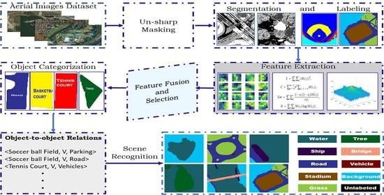
• We employed MRF as a postprocessing and labeling technique after segmentation to avoid the challenges encountered during segmentation while using other segmentation techniques, i.e., accurate scene classification.
• CNN and classical features including Haralick features, spectral-spatial features, and super-pixel patterns are fused to improve the classification accuracy.
• MKL-based categorization significantly enhances the performance of object categorization.
• Probability-based OOR relations are introduced to contextually analyze the relationship between the objects present in the remote sensing scenes.
• After object categorization and OOR exploration, FCN is applied for the remote scene classification.

The rest of the paper is organized as follows: Section 2 discusses related works. Section 3 provides an overview of the proposed method, which includes segmentation, labeling, feature extraction, and their fusion. Section 4 gives the details of the datasets used, the experimental design, and the outcomes. Lastly, in Section 5, we provide the conclusions of this study.

2. Related Work

Exploring the locations among several objects, their calibration and positioning, and the impact of scenic imagery are complicated issues in the domain of aerial and remote sensing images. We conducted a literature review across multiple domains, including object categorization, object segmentation, labeling, and scene classification to develop appropriate dynamics and metrics for the presented approach.

2.1. Object Categorization

The area of object categorization involves various challenges for researchers, including locating objects, detecting and analyzing their relationships, finding occluded components, and separating classes for desirable outcomes. Over the last decade, the bag-of-features model has undoubtedly been the most popular and effective paradigm for imagery categorization and classification. Numerous intriguing works have focused on the bag-of-features concept [14]. Martin et al. [15] developed a Bayesian inference model to assess each object’s previous knowledge to track several objects. It then revised the potential mass function to allow for more precise object recognition and convergence rate for accurate classification. In [16], they offered a unique class-specific illustration technique for object categorization. Initially, they used a Gaussian mixture model (GMM) to describe the features of images inside that class. Image and GMM models were then compared in terms of their respective Euclidean distances, which were utilized to represent each image. This was achieved by concatenating the representations of all the classes. In this method, they could express an image by combining the class-specific features, as well as the visual components. In [17], an effective technique was presented to classify the indoor–outdoor scenes by employing multi-object categorization. They used two different approaches to segment the images, and then object categorization was performed using multiple kernel learning (MKL) by considering local descriptors with the combination of signatures of a specific region. After finding the object relationships, they applied multiclass logistic regression to classify the scenes.

Wong et al. [18] presented an approach for online object detection and classification of the image’s object classes. They proposed using kernel learning to rapidly track all the objects in a scene rather than relying on past knowledge of a single object. The Neovision2 tower benchmark dataset was used to develop a biologically inspired approach for detecting an object’s contours and motion. Sumbul et al. [19] developed methods that incorporated the attention of a multisource region network that computed the pre-source feature illustration and was then distributed across the network’s members on the basis of their representations of object locations. They employed multispectral approaches to achieve better accuracy.

2.2. Scene Classification

Previously published research utilized low-level cues to categorize objects and scenes. These low-level cues include histograms of gradients [20], statistical analysis of structural information for texture discrimination [21], GIST [22], and scale-invariant feature transform (SIFT) [23]. However, these solutions depended on technical expertise and expert knowledge to generate feature representations, which have limits when it comes to representing large amounts of scene data. To overcome the shortcomings of low-level feature-based classification approaches, several approaches have been devised to improve the efficiency of scene classification by aggregating the collected local low-level visual cues into a mid-level scene illustration. One of the most extensively used systems based on mid-level visual features is bag of visual words (BoVW) [24]. It constructs a visual dictionary using k-means clustering, and mid-level visual information is extracted and achieved through feature encoding. Their model used BoVW and its advanced versions to classify scenes on numerous occasions. Additionally, some other mid-level features based on traditional approaches exist, including spatial pyramid matching [25], improved fisher kernel [26], and vectors of locally aggregated descriptors [27].

However, previously described approaches, which rely on low- and mid-level features retrieved from RS imagery, are not particularly sophisticated and, hence, cannot adequately reflect the semantic information contained in images. Recent research has demonstrated that deep learning approaches, particularly CNN, perform exceptionally well in computer vision applications due to their great feature extraction capacity. Additionally, RS image scene classification falls under the category of high-level image processing tasks that are strongly connected to computer vision. RS images have a poor resolution at an early stage, and the scenes to be identified are large-area land cover, in contrast to natural images used in computer vision, which focus on small-scale items. As a result, it has trouble incorporating deep learning-based algorithms into the categorization of RS image scenes. However, the RS images now have a high spatial resolution, while the disparity amongst RS and natural images has also been minimized; hence, the possibility of incorporating different remote sensing visualization techniques into image processing has increased. Numerous CNN-based algorithms for scene classification have been introduced recently [28]. Rather than relying on low- and mid-level cues, CNN-based approaches may extract hierarchical features from RS images. Additionally, the majority of CNN-based approaches make use of models that have been pretrained on ImageNet [29], including AlexNet [10], VGG [11], ResNet [13], and DenseNet [30]. Hu et al. [31] validated the efficiency of CNN models utilizing convolutional layer features. Li et al. suggested a unique filter bank in [32] for simultaneously capturing local and global data in order to improve the results of classification. They investigated the effect of various training procedures on the categorization process. Their system includes three different training approaches: feature extraction and fine-tuning through a pretrained CNN framework, and fully trained networks. The experimental findings revealed that, when compared to the other two procedures, the fine-tuning strategy achieved a better classification accuracy.

3. Proposed System Methodology

This section demonstrates a novel object categorization and scene classification (OCSC) model that categorizes the objects present in the remote scene imagery. Moreover, it classifies the scenes on the basis of these categorized objects. Initially, a remote sensing image is considered for segmentation by employing fuzzy C-means (FCM) algorithms. Then, these segmented objects are further processed to improve the segments and labeled via MRF. The labeled objects are then analyzed for feature extraction by CNN, while classical features including Haralick features, SSFs, and super-pixel patterns are also extracted. After the fusion of these extracted features, MKL is applied to categorize the unique objects in the remote scene images. Once the categories of the objects are separated, the OOR is computed on the basis of probability triplets. Finally, these OOR probabilities and object categories are taken as the input of FCN for remote sensing scene classification. Figure 1 illustrates the hierarchal view of our system.

3.1. Preprocessing Stage

Un-sharp masking [33] for image sharpening is performed during preprocessing to provide an enhanced image with sharp edges. Three parameters are used to produce un-sharp masking: amount, radius, and threshold. The amount parameter is used to adjust the contrast between the edges and is typically specified as a percentage. Radius defines the thickness of the edge and can be increased. A threshold is used to control the image’s brightness level. We set the radius and amount parameters to 0.75% and 1.25%, respectively, during our study. The following formula can be used to obtain a sharper image:

$$I_{sh}=I_o+\left(I_o-I_b\right)\times amt,$$

(1)

where $I_{sh}$ represents the sharpened image, $I_o$ specifies the original image, a blurred image is represented by $I_b$ and $amt$ is to describe the amount parameter which denotes the strength of the sharpening effect.

3.2. Object Segmentation via Fuzzy C-Means

This section describes the fuzzy C-means (FCM) approach [34,35] for segmentation. Initially, homologous components are spotted on the basis of pixels that are considered data points, consistent with the method. Rather than being assigned to a single defined cluster, each pixel demonstrating a fuzzy logic is then considered to be a member of numerous clusters. By iteratively minimizing the objective function, the FCM fragments the image. Additionally, these features constrain ideal image clusters by reducing cluster weights using the squared error objective function $A_N\left(P,Q\right)$ as follows:

$$A_N\left(P,Q\right)={{\displaystyle \sum }}_{i=1}^c{{\displaystyle \sum }}_{j=1}^n{p}_{ij}^r{\left|x_j-q_i\right|}^2,$$

(2)

where $n$ illustrates the number of data points with $r$ real numbers in the i-th cluster, c denotes the clusters, $p_{ij}^r$ reflects the membership of $x_j$ pixels in the i-th cluster, and $q_i$ expresses the centroid of the cluster.

$$p_{ij}=\frac{1}{{{\displaystyle \sum }}_{k=1}^c{\left(\frac{\left|x_j-q_i\right|}{{\left|x_j-q_k\right|}^2}2\right)}^{\frac{1}{r-1}}},$$

(3)

$$p_{ij}\in \left[0,1\right], \mathrm{for} i=\left[1,\dots ,c\right],$$

(4)

$$q_i=\frac{{{\displaystyle \sum }}_{j=1}^n{p}_{ij}^r{x}_j}{{{\displaystyle \sum }}_{j=1}^n{p}_{ij}^r},$$

(5)

where $A_N\left(P,Q\right)$, the distance between each pixel and the cluster center, may be calculated using $P$ and $Q$. When the minimal distance from the pixel to the cluster center is observed, a high membership value is allocated to the well-suited pixel. Using the typical FCM approach, a high level of computational complexity is produced because of the analysis of spatial values at each iteration that is used to quantify the distance from the cluster center to the relevant pixel in an image. Figure 2 shows the outcomes of segmenting the images from the UCM dataset.

3.3. Labeling via Markov Random Field

A Markov random field (MRF) [36,37] can be described in formal terms by a set of sites S = {1, …, N}. These are N pixel places. A collection of random variables ${\left\{w_n\right\}}_{n=1}^N$ and a set of neighbors ${\left\{{\mathcal{N}}_n\right\}}_{n=1}^N$ are connected with each of the N locations. To qualify as a Markov random field, the model must adhere to the following Markov property:

$$\mathrm{Pr}\left(w_n\mid w_{\mathcal{S}\backslash n}\right)=\mathrm{Pr}\left(w_n\mid w_{{\mathcal{N}}_n}\right).$$

(6)

As a result, a Markov random field (MRF) can be considered to be an undirected model that specifies the conditional probabilities of variables as a product of potential functions such that

$$\mathrm{Pr}\left(w\right)=\frac{1}{Z}{{\displaystyle \prod }}_{j=1}^J{\varphi }_j\left[{\mathrm{w}}_{{\mathcal{C}}_j}\right],$$

(7)

where ϕ_j [•] is the j-th potential function, which never yields a negative value. This value is determined by the state of a subset of the variables ${\mathcal{C}}_j$ ⊂ {1, …, N}. This subset is referred to as a clique in this context. The partition function, denoted by $Z$, is a normalizing constant that ensures the resulting probability distribution is correct. We used MRF for postprocessing of segmented regions. The segmented regions having discontinuities are initially connected by considering the multiple key points on boundaries and connecting these key points to accurately separate the segmented regions. Then, these regions with a boundary around the connected regions having pixels with similar features are grouped together and assigned a unique label. Figure 3 illustrates the results of MRF labeling on a selection of images from the AID. Figure 3 illustrates the results of MRF labeling on a selection of images from the AID.

3.4. Feature Extraction

To categorize the objects in remote sensing imagery, various classical and deep features are analyzed. Classical features including Haralick texture features, SSFs, and super-pixel patterns are computed on the basis of statistical techniques while deep learning-based features are extracted using a pretrained CNN model. This section covers the feature computation, fusion, and selection processes in detail.

3.4.1. CNN Features

To extract CNN features [38], VGG-16 (a pretrained CNN model) is incorporated. Deng et al. [39] trained this model on the ImageNet dataset. The model is simple and comprises an input layer and 13 convolutional layers. The input layer considers the images with dimensions of 320 × 320 × 3 as input. There are also five pooling layers (max pooling) following the three fully connected layers. The window size for max-pooling is 2 × 2. The rectified linear unit (ReLU) is used as an activation function in hidden layers. To extract effective CNN features, a transfer learning method is applied that exploits the already learned features to make the model useful as compared to training a new model from scratch. The general architecture of CNN features extraction is shown in Figure 4.

3.4.2. Haralick Features

Remote sensing images of several objects may appear identical in color but have distinct texture patterns. This inspired us to integrate texture features that behave as local descriptors. To obtain texture features, we used a cooccurrence matrix. The four local features are derived from a matrix of cooccurrences termed Haralick features [40]. Haralick assumed that this matrix contains texture information, and texture features are subsequently computed from this matrix. The cooccurrence matrix contains 14 factors; however, only four are commonly used. These four texture features, energy ($E$), contrast ($C$), correlation ($\mathrm{Cor}$), and entropy ($H$), are computed mathematically by the following equations:

$$E={{\displaystyle \sum }}_i{{\displaystyle \sum }}_j{(M\left(i,j\right))}^2,$$

(8)

$$C={{\displaystyle \sum }}_{k=0}^{m-1}{k}^2{{\displaystyle \sum }}_{\left|i-j\right|=k}M\left(i,j\right),$$

(9)

$$\mathrm{Cor}={{\displaystyle \sum }}_i{{\displaystyle \sum }}_j\frac{\left(i-{\mu }_i\right)\left(j-{\mu }_j\right)M\left(i,j\right)}{{\sigma }_i{\sigma }_j},$$

(10)

$$H={{\displaystyle \sum }}_i{{\displaystyle \sum }}_{j}M\left(i,j\right)\log \left(M\left(i,j\right)\right).$$

(11)

It was demonstrated that these four parameters were sufficient to produce acceptable results in a classification test. These four parameters are listed with their values in

Table 1. Attribute values of different Haralick features for labeled objects compared with GT with errors on AID.

Objects	Evaluation	Features
		Contrast	Energy	Entropy	Correlation
Tennis Court	GT	121,334	0.2151	0.2053	0.8905
	SG	130,774	0.2108	0.2175	0.8917
	ER	±9440	±0.0043	±0.0122	±0.0012
Ship	GT	191,428	0.1919	0.4401	0.7926
	SG	191,854	0.1961	0.4458	0.7811
	ER	±426	±0.0042	±0.0057	±0.0115
Soccer Field	GT	169,883	0.7205	0.3933	0.4577
	SG	160,125	0.7163	0.3875	0.4612
	ER	±9758	±0.0042	±0.0058	±0.0035
Vehicles	GT	102,657	0.4229	0.3166	0.5926
	SG	108,941	0.4195	0.3192	0.5933
	ER	±6284	±0.0034	±0.0026	±0.0007

GT = ground truth; SG = segmented; ER = error.

.

3.4.3. Spectral–Spatial Features (SSFs)

Mathematical morphology [41] is one of the well-known paradigms that equips operators with the ability to generate high-quality SSFs [42]. Erosion and dilation are basic mathematical morphology operations that examine an image’s geometrical structures by comparing them to small patterns called structuring elements.

Attribute filters (AF): Various flat regions of the image, or areas of the image that have comparable gray levels are used to extract various types of information, specified by the feature names. An image’s equivalent tree representation can be used to effectively build attribute filters as in [43]. By applying a threshold to all of the image’s mapped values, the following sets of higher- and lower-level sets (i.e., flat zones) are created that can be further classified into subcategories:

$$\begin{array}{c}U\left(f\right)=\left\{X:X\in Con\mathcal{C}omp\left(\left[f\ge \lambda \right]\right),\lambda \in Z\right\}\\ L\left(f\right)=\{X:X\in Con\mathcal{C}omp([f<\lambda ]),\lambda \in Z\}\end{array},$$

(12)

where $Con\mathcal{C}omp$ denotes the connected components of the generic image. An inclusion relationship [33] exists between the interconnected components that are obtained by either the lowest- or the highest-level sets.

Attribute profiles (APs): APs define a generic collection of profiles that make use of the attribute filter’s flexibility to conduct a more thorough investigation of the scene.

Extended attribute profiles: Because hyperspectral sensors acquire data across many spectral bands, extended attribute profiles (EAPs) based on morphological attribute filters are used to analyze hyperspectral high-resolution images. The EAPs are based on the application of the APs to hyperspectral data.

$$EAP=\left\{AP\left(P{C}_1\right),AP\left(P{C}_2\right),\dots ,AP\left(P{C}_c\right)\right\},$$

(13)

where $PC$ denotes one principal component obtained by applying principal component analysis to the data.

Extended multi-attribute profiles (EMAPs): Many features can be used to extract spatial elements more effectively; hence, EMAPs combine multiple EAPs into a single data structure.

$$\left.EMAP=\{EA{P}_{a_1},EA{P}_{a_2}^{\prime },\dots ,EA{P}_{a_m}^{\prime }\right\}.$$

(14)

The spatial information extraction in the EMAP is substantially more powerful than a single EAP; however, processing these features incurs a substantial cost in terms of computation, as the max-tree and min-tree are generated just once for each $PC$ and are processed with various attributes at multiple stages. The visual results of SSFs over areal images are presented in Figure 5.

3.4.4. Super-Pixel Pattern

We present a method for creating super-pixels following [44] that is faster and more memory-effective than current approaches. It demonstrates state-of-the-art boundary conformance and enhances the segmentation efficiency. Simple linear iterative clustering is a modification of k-means for super-pixel creation, with two critical differences: the first one is reducing optimization time by narrowing the search area based on super-pixel size, which leads to significantly fewer distance calculations, and the second one describes that there is no dependence of the number of super-pixels k on how many pixels N there are; hence, the complexity is reduced to a linear function. It is possible to regulate the size and coherence of the super-pixels using color and spatial distance combined as a weighted distance metric.

Super-pixels correspond to clusters in color-image plane space. This causes an issue in determining the distance measure $Dis{t}_F$. To compute the distance between a pixel i and cluster center $C_k$, distance measure $Dis{t}_F$ is used. A color space ${[l a b]}^{\mathrm{T}}$ having a range of known values is considered for color representation of every pixel. The pixel’s position${\left[\begin{array}{c}x\hspace{0.17em}\hspace{0.17em}\hspace{0.17em}\hspace{0.17em}y\end{array}\right]}^T$, on the other hand, may take a range of values that vary according to the size of the image. We need to compute two distances, i.e., normalized color distance and spatial distance. We then combine these two distances into a single measure by their respective maximum distances within a cluster, $No{r}_{spt}$ and $No{r}_{col}$. In doing so, $Dis{t}_F$ is written as

$$\begin{array}{c}dis{t}_{col}=\sqrt{{\left(l_j-l_i\right)}^2+{\left(a_j-a_i\right)}^2+{\left(b_j-b_i\right)}^2},\\ dis{t}_{spt}=\sqrt{{\left(x_j-x_i\right)}^2+{\left(y_j-y_i\right)}^2},\\ Dis{t}_F=\sqrt{{\left(\frac{d_c}{No{r}_{col}}\right)}^2+{\left(\frac{d_s}{No{r}_{spt}}\right)}^2}.\end{array}$$

(15)

Results of super-pixel patterns computed over some remote sensing images from UCM dataset are presented in Figure 6.

3.5. Feature Fusion

The CNN, Haralick features, SSFs, and super-pixel patterns are computed separately as $Featur{e}_{CNN}$, $Featur{e}_{Haralick}$, $Featur{e}_{SS}$, and $Featur{e}_{SP}$, respectively. All these feature vectors are merged as in [45] to form a complete fused feature vector and normalized before fusion, to ensure that the individual feature vectors elements do not surpass other elements. Once normalization is performed, the CNN, Haralick, SSF, and super-pixel patterns are pooled to form a complete fused feature vector.

$$Featur{e}_F=\left[Featur{e}_{CNN} Featur{e}_{Haralick} Featur{e}_{SS} Featur{e}_{SP}\right].$$

(16)

A high-dimensional feature vector is obtained as a result of the two-level decomposition of complex images while feature analysis is executed. Consequently, an inadequate classification is witnessed when the input feature vectors have high dimensions. Therefore, reducing the size of feature vectors is important in order to reduce computational costs and improve performance. For the purpose, GA-based [46] feature selection is employed to obtain the reduced dimensional feature vector $Featur{e}_{Fin}$:

$$Featur{e}_{Fin}=GA\left[Featur{e}_F\right].$$

(17)

3.6. Object Categorization: Multiple Kernel Learning

The proposed system employs MKL [17] to achieve object categorization on the basis of multiple regions and signatures of the regions in complex remote sensing imagery, as shown in Figure 7. During object categorization, an image $I$ having a number of $c$ clusters obtained from the segmented and labeled objects that are presented in various distinct colors is taken to extract descriptor $D_I$, which describes the region R of the image I. Now, to compute the signature $x_I$, a function $f_R$ from local descriptors $D_I$ as $f_R:D_I\to x_I$ is incorporated. Mathematically, $f_R$ can be written as follows:

$$Cente{r}_c=\frac{1}{\left|c\right|}{{\displaystyle \sum }}_I{{\displaystyle \sum }}_i{D}_{icI},$$

(18)

$${\mu }_c=\frac{1}{\left|c\right|}{{\displaystyle \sum }}_I{{\displaystyle \sum }}_i\left(D_{icI}-Cente{r}_c\right){\left(D_{icI}-Cente{r}_c\right)}^{\top },$$

(19)

$${\mu }_{I,c}={{\displaystyle \sum }}_i\left(D_{icI}-Cente{r}_c\right){\left(D_{icI}-Cente{r}_c\right)}^{\top }-{\mu }_c,$$

(20)

where $Cente{r}_c$ represent clusters center c, entire descriptors are described by |c| in the clusters c for all the images from a class, descriptors of image I that belong to cluster c are shown as $D_{icI}$, and the mean of those centered descriptors belonging to c is denoted by ${\mu }_c$, while ${\mu }_{j,c}$is the signature computed from the image I. Then, a vector $VE{C}_{I,C}$ is obtained from ${\mu }_{I,c}$. The computation of signature vector $x_I$ of image I for all c is performed by the concatenation of all $VE{C}_{I,C}$.

$$VE{C}_I=\left(VE{C}_{I,1}\dots VE{C}_{I,C}\right).$$

(21)

3.7. Probability-Based Object-to-Object Relations (OORs)

After recognition of multiple objects in a complex scene, the relationship between these objects is identified. To enhance the scene recognition performance, object-to-object relations (OORs) [47] are computed on the basis of contextual information regarding objects. As complex scenes comprise multiple co-occurring visual features, these OORs significantly recognize patterns to understand the scenes. For instance, a car is likely to be seen on roads instead of the sky or water, while a ship is likely to be in the sea or water instead of on roads. To determine the OORs, several features and relative positions of the objects are considered. Initially, to find the weight of the $j$-th target object for $j \in \left\{1, 2, \dots , n\right\}$ with respect to another relevant $i^{}$-th object for $i\in \left\{1, 2, \dots , n\right\}$, a dot product is computed as follows:

$$w_t\left(j,i\right)=\frac{f_j\cdot f_i}{d\left(j,i\right)},$$

(22)

where the visual cures of the $j^{}$-th and $i^{}$-th object are represented by $f_j$ and $f_i$, respectively. The distance between the $j^{}$-th and $i^{}$-th object is denoted by (j, i). Lastly, to determine the relation of the $j^{}$-th object with other objects, the following expression is used:

$$R_j={{\displaystyle \sum }}_i{w}_t\left(j,i\right)\cdot f_i^n,$$

(23)

where the visual features of the $i^{}$-th object are denoted by $f_i^n$. While the relations are computed between the objects, the scene labels are predicted by the classifier on the basis of these OORs. Figure 8 presents a schematic view of OORs.

3.8. Scene Recognition: Fully Convolutional Network

Once the OOR is determined, object triplets and probabilities are forwarded to the FCN that classifies the scenes by incorporating the object category and contextual relationship between those objects. FCN [48] is an architecture that is mostly used for semantic segmentation. FCN employs locally connected layers, including convolution, pooling, and up-sampling, in a variety of ways. Avoiding dense layers results in fewer parameters (i.e., making the networks faster to train). Additionally, because all connections are local, an FCN can be used with varying image sizes. The network is composed of a down-sampling path for extracting and interpreting context, as well as an up-sampling path for localization.

A fully convolutional network (FCN) with the following hyperparameters is used to classify the remote sensing scenes: a learning rate of 0.01, a batch size of 16, and 32 conv_block1 filters, 64 conv_block2 filters, 128 conv_block3 filters, 264 conv_block4 filters, and 512 conv_block5 filters. Although we could choose a learning rate with a floating-point value between 0.0001 and 0.1, a learning rate of 0.01 led to the best results during our training process for remote scene classification over the benchmark datasets under consideration, i.e., UCM, AID, and RESISC45 datasets. Similarly, the batch size can range from 1–100, but the power of 2 is mostly chosen as the batch size; we chose 16 (2⁴) following its better performance during training. Figure 9 depicts the results of scene classification on a benchmark dataset.

4. Experimental Results

To evaluate the training/testing performance of the proposed model, we used the leave-one-out cross-validation method on three publicly available datasets: AID, RESIEC45 dataset, and UCM dataset.

4.1. Datasets Description

4.1.1. Aerial Images Dataset

The Aerial Images Dataset (AID) [49] is a newly created large-scale aerial image collection. The AID comprises 30 classes having 10,000 images. Each class is composed of 200–400 images, and every image contains at least two objects and at most eight objects. The dataset covers the following aerial scene types: airport, bare land, baseball field, beach, bridge, center, church, commercial, dense residential, desert, farmland, forest, industrial, meadow, medium residential, mountain, park, parking, playground, pond, port, railway station, resort, river, school, sparse residential, square, stadium, and viaduct. Figure 10 presents some example images from the AID.

4.1.2. RESISC45 Dataset

The RESISC45 dataset [50] is one of the well-known benchmarks for remote sensing image scene classification. This dataset was created by Northwestern Polytechnical University (NWPU); therefore, it is also named NWPU-RESISC45, and it consists of 31,500 remote sensing images of 45 various scene classes. Each class comprises 700 images with a minimum of two and maximum of 10 objects in each class. These classes are airplane, airport, basketball diamond, baseball court, beach, bridge, forest, golf course, etc. Figure 11 shows a few classes of he f NWPU-RESISC45 dataset.

4.1.3. UCM Dataset

The UCM dataset [51] is a benchmark that is publicly available for research purposes. The dataset comprises 21 classes with 100 images in each class. The number of objects in each class may vary from two to seven depending on the class scenario. The dimensions of the images are 256 × 256 pixels. For several cities across the country, the USGS National Map Urban Area Imagery collection was used to manually extract the imagery. The classes are labeled as agricultural, airplane, baseball diamond, beach, buildings, chaparral, dense residential, forest, freeway, golf course, harbor, intersection, medium residential, mobile home park, overpass, parking lot, river, runway, sparse residential, storage tanks, and tennis court. Figure 12 illustrates a few examples of the UCM dataset.

4.2. Experimental Evaluation

In this section, we present the recognition accuracies based on the confusion matrices computed over three complex datasets: the AID, UCM dataset, and RESISC45 dataset. For OCSC, we used an FCN as a classifier, and the proposed system was evaluated by the leave-one-subject-out (LOSO) cross-validation technique. Figure 13 demonstrates the results over the UCM dataset with an average of 98.75% scene classification accuracy. Figure 14 presents a classification accuracy of 97.73% over the AID, and Figure 15 demonstrates an average accuracy of 96.57% over the RESISC45 dataset.

Class-wise accuracies may be studied with the color code against each class label on the left of the graph, which is specified for the corresponding class. The mixture of different colors on the right denotes different classes present in the result which may be encoded as misclassification. Misclassification is interpreted as a color in the graph line above that specific class, which is a false positive (FP), or a color in the mixture below the original class, which is a false negative (FN). For instance, the FL class in the AID shows both FPs and FNs in the graph along with correct predictions, where CH and DS are FPs, while FR and IN are FNs shown in the graph.

The recognition results of the UCM dataset show that GC, HB, and PG had lower accuracies compared to other scene classes. However, the overall recognition accuracy was better and comparable with other state-of-the-art methods. There are a total of 21 classes in the UCM dataset; out of those, we achieved remarkable performance on 18 classes, while the other three classes had good results, nearly equivalent to other existing methods.

Similar to the UCM dataset, we observed better performance over the AID compared to other SOTA techniques, as presented in Figure 14. Most of the classes demonstrated remarkable results in terms of accuracy. Higher accuracy was achieved by more than 20 classes including RV, SQ, SM, ST, and VD, while some other classes (DR, DS, FL, and PD) still need improvement. For instance, the IN class achieved an accuracy of 90% as shown in Figure 14, which demonstrates that 2% of cases were incorrectly recognized as FL and 8% of cases were misclassified as “DS”. Likewise, class-wise accuracies may be studied with the color against each class label on the left of the graph, where a mixture of different colors on the right denotes misclassification.

Analogous to that of the UCM and AID, the OCSC model demonstrated excellent performance when evaluated over the RESISC45 dataset. Figure 15 illustrates that most of the classes depicted exceptional performance in terms of recognition accuracy including PG and MW with accuracies of 99%, where MW was misclassified 1% of the time as MK, while the lowest accuracy was noted for the CL class, where CL was misclassified as CM, DR, and DS 9%, 8%, and 4% of the time, respectively.

In this section, experimental evaluation was performed on benchmarks including the AID, UCM dataset, and RESISC45 dataset. At first, the CNN and classical features (i.e., SSFs, Haralick features, and super-pixel patterns) were given to the most commonly used classifier artificial neural network (ANN), and its results were obtained. Then, the same features were given to a deep belief network (DBN) for recognition. Finally, a comparison of the recognition results using conventional approaches with that of the proposed OCSC model using FCN was performed.

Table 2. Scene classification results against three classifiers on AID.

Classes	ANN			DBN			FCN (Ours)
	Precision	Recall	F1 Score	Precision	Recall	F1 Score	Precision	Recall	F1 Score
AP	0.768	0.732	0.75	0.811	0.855	0.832	0.901	0.977	0.937
BL	0.883	0.765	0.82	0.754	0.815	0.783	0.965	0.965	0.965
BB	0.691	0.813	0.747	0.688	0.755	0.72	0.824	0.972	0.892
BH	0.724	0.798	0.759	0.617	0.845	0.713	0.977	0.911	0.943
BR	0.817	0.841	0.829	0.754	0.933	0.834	0.899	0.931	0.917
CC	0.677	0.875	0.763	0.725	0.841	0.779	0.891	0.889	0.89
CM	0.755	0.839	0.795	0.697	0.798	0.744	0.915	0.787	0.846
DR	0.695	0.759	0.726	0.711	0.899	0.794	0.872	0.854	0.911
DT	0.786	0.698	0.739	0.695	0.884	0.778	0.928	0.971	0.949
FL	0.695	0.764	0.728	0.654	0.815	0.726	0.971	0.892	0.93
FR	0.754	0.856	0.802	0.632	0.856	0.727	0.915	0.977	0.945
IN	0.655	0.813	0.725	0.719	0.796	0.756	0.811	0.892	0.85
MW	0.771	0.792	0.781	0.705	0.862	0.776	0.913	0.928	0.92
MR	0.798	0.733	0.764	0.733	0.784	0.758	0.986	0.966	0.976
MN	0.699	0.795	0.744	0.826	0.698	0.757	0.897	0.937	0.917
PK	0.784	0.875	0.827	0.798	0.814	0.806	0.912	0.901	0.906
PG	0.789	0.839	0.813	0.771	0.761	0.766	0.977	0.887	0.93
PD	0.681	0.821	0.744	0.811	0.886	0.847	0.799	0.916	0.854
PN	0.719	0.788	0.752	0.631	0.818	0.712	0.855	0.891	0.873
RS	0.725	0.811	0.766	0.801	0.875	0.836	0.925	0.917	0.921
RT	0.774	0.859	0.814	0.783	0.836	0.809	0.936	0.977	0.956
RV	0.615	0.694	0.652	0.697	0.825	0.756	0.871	0.871	0.871
SL	0.664	0.851	0.746	0.665	0.851	0.747	0.995	0.951	0.973
SR	0.776	0.785	0.78	0.709	0.898	0.792	0.956	0.879	0.916
SQ	0.764	0.809	0.786	0.722	0.835	0.774	0.891	0.903	0.897
SM	0.687	0.717	0.702	0.715	0.746	0.73	0.819	0.916	0.865
ST	0.694	0.839	0.76	0.812	0.816	0.814	0.977	0.921	0.948
VT	0.639	0.775	0.7	0.789	0.857	0.822	0.887	0.911	0.899
AP	0.715	0.795	0.753	0.745	0.877	0.806	0.973	0.935	0.954
BL	0.636	0.699	0.666	0.781	0.798	0.789	0.985	0.905	0.943
Mean	0.728	0.794	0.758	0.732	0.831	0.776	0.914	0.921	0.916

,

Table 3. Scene classification results against three classifiers on RESISC45 dataset.

Classes	ANN			DBN			FCN (Ours)
	Precision	Recall	F1 Score	Precision	Recall	F1 Score	Precision	Recall	F1 Score
AP	0.611	0.874	0.719	0.622	0.717	0.666	0.901	0.977	0.937
AT	0.637	0.769	0.697	0.783	0.865	0.822	0.899	0.845	0.871
BD	0.712	0.825	0.764	0.759	0.786	0.772	0.995	0.951	0.973
BC	0.698	0.813	0.751	0.768	0.937	0.844	0.986	0.915	0.949
BG	0.672	0.749	0.708	0.651	0.831	0.757	0.967	0.903	0.934
BH	0.655	0.875	0.749	0.748	0.875	0.807	0.844	0.869	0.859
BR	0.751	0.839	0.793	0.879	0.831	0.854	0.871	0.839	0.855
CL	0.697	0.781	0.737	0.728	0.729	0.728	0.872	0.921	0.896
CH	0.743	0.829	0.784	0.688	0.866	0.767	0.886	0.938	0.911
CF	0.779	0.787	0.783	0.825	0.781	0.802	0.985	0.954	0.969
CD	0.702	0.854	0.771	0.716	0.698	0.707	0.901	0.977	0.937
CA	0.699	0.772	0.734	0.803	0.865	0.833	0.883	0.965	0.922
DR	0.785	0.801	0.793	0.776	0.758	0.767	0.995	0.951	0.973
DT	0.734	0.791	0.761	0.868	0.801	0.833	0.986	0.937	0.961
FT	0.709	0.767	0.737	0.689	0.774	0.729	0.967	0.903	0.934
FW	0.664	0.775	0.715	0.791	0.875	0.831	0.844	0.861	0.852
GC	0.637	0.739	0.684	0.711	0.839	0.770	0.977	0.839	0.903
GT	0.649	0.812	0.721	0.782	0.881	0.829	0.872	0.921	0.896
HR	0.711	0.738	0.724	0.686	0.787	0.733	0.886	0.938	0.911
IA	0.753	0.813	0.782	0.658	0.824	0.732	0.985	0.954	0.969
IN	0.668	0.745	0.704	0.854	0.761	0.805	0.901	0.977	0.937
ID	0.622	0.851	0.719	0.783	0.824	0.803	0.883	0.965	0.922
LK	0.677	0.751	0.712	0.852	0.699	0.768	0.995	0.951	0.973
MD	0.711	0.825	0.764	0.755	0.785	0.770	0.986	0.937	0.961
MR	0.787	0.694	0.738	0.677	0.823	0.743	0.967	0.903	0.934
MH	0.689	0.785	0.734	0.711	0.785	0.746	0.844	0.875	0.859
MN	0.791	0.839	0.814	0.816	0.819	0.817	0.977	0.839	0.903
OP	0.698	0.789	0.741	0.794	0.895	0.841	0.872	0.851	0.861
PC	0.655	0.818	0.727	0.729	0.852	0.786	0.886	0.938	0.911
Pk	0.785	0.755	0.770	0.688	0.815	0.746	0.985	0.954	0.969
RL	0.709	0.745	0.727	0.645	0.758	0.697	0.967	0.903	0.934
RS	0.615	0.698	0.654	0.731	0.775	0.752	0.844	0.875	0.859
RF	0.822	0.739	0.778	0.779	0.881	0.827	0.977	0.839	0.903
RV	0.746	0.699	0.722	0.745	0.721	0.733	0.872	0.921	0.896
RT	0.699	0.811	0.751	0.654	0.819	0.727	0.886	0.938	0.911
RN	0.775	0.782	0.778	0.697	0.754	0.724	0.985	0.954	0.969
SI	0.716	0.757	0.736	0.725	0.688	0.706	0.901	0.977	0.937
SH	0.883	0.765	0.82	0.811	0.669	0.733	0.883	0.965	0.922
SB	0.788	0.801	0.794	0.735	0.715	0.725	0.995	0.951	0.973
SR	0.811	0.735	0.771	0.824	0.689	0.750	0.986	0.937	0.961
SD	0.699	0.619	0.657	0.755	0.745	0.751	0.967	0.903	0.934
ST	0.754	0.785	0.769	0.846	0.778	0.811	0.844	0.875	0.859
TC	0.768	0.838	0.801	0.661	0.829	0.736	0.977	0.839	0.903
TR	0.872	0.721	0.789	0.693	0.818	0.75	0.872	0.921	0.896
TP	0.689	0.738	0.713	0.778	0.736	0.756	0.886	0.938	0.911
WD	0.661	0.654	0.657	0.688	0.744	0.715	0.985	0.954	0.969
Mean	0.735	0.794	0.761	0.763	0.813	0.784	0.947	0.939	0.942

and

Table 4. Scene classification results against three classifiers on UCM dataset.

Classes	ANN			DBN			FCN (Ours)
	Precision	Recall	F1 Score	Precision	Recall	F1 Score	Precision	Recall	F1 Score
AG	0.837	0.658	0.737	0.699	0.899	0.787	0.967	0.903	0.934
AP	0.755	0.788	0.811	0.815	0.875	0.844	0.844	0.875	0.860
BD	0.792	0.753	0.815	0.741	0.819	0.787	0.977	0.839	0.903
BH	0.873	0.707	0.781	0.784	0.944	0.857	0.872	0.921	0.896
BG	0.799	0.791	0.795	0.785	0.859	0.821	0.886	0.938	0.912
CP	0.701	0.825	0.758	0.667	0.769	0.715	0.985	0.954	0.970
DR	0.766	0.811	0.788	0.719	0.688	0.704	0.901	0.977	0.938
FR	0.783	0.711	0.746	0.883	0.965	0.923	0.809	0.951	0.881
FW	0.699	0.764	0.731	0.792	0.881	0.835	0.995	0.951	0.973
GC	0.715	0.795	0.753	0.763	0.896	0.825	0.986	0.937	0.961
HB	0.855	0.801	0.828	0.648	0.821	0.725	0.967	0.903	0.934
IS	0.785	0.815	0.828	0.791	0.798	0.795	0.844	0.875	0.860
MR	0.821	0.802	0.83	0.737	0.809	0.772	0.977	0.839	0.903
MP	0.787	0.655	0.715	0.783	0.898	0.837	0.872	0.921	0.896
OP	0.845	0.669	0.747	0.897	0.762	0.825	0.886	0.938	0.912
PG	0.769	0.759	0.764	0.799	0.711	0.753	0.985	0.954	0.970
RV	0.811	0.661	0.729	0.675	0.855	0.755	0.967	0.903	0.934
RW	0.845	0.716	0.776	0.795	0.789	0.79	0.844	0.875	0.860
SR	0.775	0.797	0.806	0.819	0.773	0.796	0.977	0.839	0.903
ST	0.771	0.824	0.797	0.719	0.898	0.799	0.872	0.921	0.896
TC	0.786	0.891	0.836	0.801	0.795	0.798	0.886	0.938	0.912
Mean	0.789	0.777	0.783	0.768	0.835	0.801	0.919	0.913	0.916

present the comparison results of precision, recall, and F1 Score over the AID, RESISC45 dataset, and UCM dataset, respectively.

In this section, we present the precision, recall, and F-1 measures computed over three complex datasets, the AID, UCM dataset, and RESISC45 dataset. We applied ANN and DBN for the remote sensing scene classification and compared the results with FCN (proposed) model. Although there were some comparable results in a few classes over the AID, we overall observed a significant improvement compared to the other well-known classifiers. A few classes including BR and DR showed better recall using DBN, while PD had better precision using DBN; however, results were overall excellent in all classes using the proposed model. Similarly, the mean values of precision, recall, and F1 score were highest when applying FCN (proposed model).

A similar pattern was observed when we applied three different classifiers over the RESISC45 dataset. We experienced a better precision value for BR and ST classes, while AT, BC, BH, FW, and OP classes had better recall value compared to the proposed method when a DBN was applied to the same dataset. Nevertheless, the mean precision, recall, and F1 score were the highest amongst the three well-known classifiers.

For a comprehensive evaluation, we compared the proposed system with various existing state-of-the-art (SOTA) methods including the self-attention feature selection module represented by SAFENet [52], label augmentation via ResNet18 + LA + KL [53], ACNet [54] for exploring local and global features integrated with some attention techniques for remote scene classification, ARCNet-VGGnet16 [55], Deep Fusion [56] using two-stream deep architecture for high-resolution aerial images classification, Fusion by Addition [57], and Siamese ResNet50 [58]. We compared the mean accuracy of scene classification, and the results are illustrated in

Table 5. Comparison of scene classification accuracies of SOTA methods with the proposed OCSC model.

Author/Method	Mean Accuracy %
	AID Dataset	UCM Dataset	RESIEC Dataset
SAFENet [52]	86.91 + 0.44	86.79 + 0.33	81.32 + 0.62
ResNet18 + LA + KL [53]	96.52	99.21	95.26
DBSNet [59]	92.93	97.90	--
CaffeNet [49]	89.53 ± 0.31	95.02 ± 0.81	--
GoogLeNet [49]	86.39 ± 0.55	94.31 ± 0.89	--
VGG-VD1-16 [49]	89.64 ± 0.36	95.21 ± 1.20	--
Deep Fusion [56]	94.58	98.02	--
Fusion by Addition [57]	91.87	97.42	--
Siamse ResNet50 [58]	--	94.29	95.95
Proposed	97.73	98.75	96.57

. It is demonstrated that the boosted performance of our proposed OCSC system outperformed the other reported methods in terms of mean accuracy. Specifically, comparing BoVW and SAFENet depicts an increase in the accuracy of scene classification that validates the effectiveness of feature fusion in our model. Furthermore, there is also an increase in the scene classification accuracy compared to ACNet over the AID and FESIEC45 dataset, although somewhat low but comparable accuracy was observed on the UCM dataset.

4.3. Ablation Study

We presented various features including CNN, Haralick, spectral-spatial, and super-pixel patterns. Here, we discuss the focal point of whether each of the features adds something new to the system to determine if all these features are essential for the OCSC system. To answer this, we conducted experiments to validate the influence of feature fusion and used a greedy approach that incrementally added features to our system starting with the best ones, i.e., CNN. Initially, we started experiments with CNN features only and achieved scene recognition accuracies of 91.37%, 91.88%, and 90.55% over the AID, UCM dataset, and NWPU-RESISC45 dataset, respectively. Then, we added super-pixel patterns and fused them with CNN features, observing significantly enhanced performance from 91.37% to 92.69% for AID, 91.88% to 93.19% for the UCM dataset, and 90.55% to 93.57% for the NWPU-RESISC45 dataset. The improved performance motivated us to further increase the number of features, similarly to the fusion of CNN and super-pixel patterns (SPPs) demonstrated earlier. Next, we conducted experiments with the addition of SSFs to the previously fused set of features. Fusion of SSFs to the already fused features set of CNN and SPP produced better results in terms of accuracy compared to the results obtained by previously fused features. An increase in the performance of recognition accuracy was witnessed from 92.69% to 94.19%, 93.19% to 94.99%, and 93.57% to 95.25% over the AID, UCM dataset, and NWPU-RESISC45 dataset, respectively. Therefore, we fused another classical feature, Haralick feature, with the already fused version of features and performed experiments for object categorization and scene classification. Combining all the features produced the best recognition performance with overall recognition accuracies of 97.73%, 98.75%, and 96.57% for the AID, UCM dataset, and NWPU-RESISC45 dataset, respectively. Figure 16 demonstrates the effectiveness of features while incorporating a greedy approach for feature fusion over different benchmark datasets for scene classification.

It is clear from the results presented in the Figure 16 that fusion of CNN and classical features produced comparative results to CNN. This was a bit different for the UCM dataset, where our approach had less but acceptable accuracy when considering the computational complexity of both techniques. The well-known CNN models are computationally complex compared to FCM. The details of computational time are illustrated in

Table 6. Computation time comparison of proposed segmentation technique with CNN over benchmark datasets.

Algorithm/Method	Dataset	FCM	FCM + MRF	CNN
Average computation time (s)	UCM	57.7 × 21 = 1211.7	85.1 × 21 = 1787.1	86.9 × 21 = 1824.9
	AID	61.5 × 30 = 1845.0	87.9 × 30 = 2637.0	88.5 × 30 = 2655.0
	RESISC45	67.1 × 45 = 3019.5	91.5 × 45 = 4117.5	92.8 × 45 = 4176.0

. We tested these algorithms on an Intel system with 32 GB RAM and Intel (R) Core (TM) i7-1065G7 CPU @ 1.30 GHz 1.50 GHz, along with an NVIDIA GeForce GPU. The proposed model had the least computational time required for the segmentation of remote sensing images compared to CNN.

5. Discussion

The proposed OCSC was designed to achieve object categorization and scene recognition over remote sensing imagery. In this article, we developed a framework that uses FCM for the segmentation of RS images and MRF for labeling of the segmented images. The labeled images were then further analyzed for extraction of features including CNN features and classical features (Haralick features, Spectral–spatial features, super-pixel patterns). Here, CNN features were extracted using a pretrained CNN model (VGG16), while classical features were extracted through machine learning techniques and mathematical formulation. These extracted features were then combined using a parallel fusion mechanism and optimized before transmitting to MKL as input, where various categories of objects were specified. Once the objects were categorized, the object-to-object relationship was determined, and a fully convolutional network was employed to classify the scenes.

Initially, the segmentation process is the fundamental module to properly classify remote sensing imagery. Therefore, an effective mechanism of FCM segmentation was incorporated to achieve significant results for segmented regions from the complex high-resolution scene images. After obtaining segmented regions, as a postprocessing step, an MRF was applied to obtain the labeled objects for further processing of feature extraction. During this labeling phase, the segmented regions were analyzed on the basis of the regions (connected, disconnected), and postprocessing was performed to more accurately isolate the boundaries of the regions segmented in the previous phase. These improved segmented regions were then labeled on the basis of a perceptual grouping mechanism, where each segmented region was assigned with a unique label (color).

This complementary module for labeling significantly enhanced the object categorization. We conducted experiments for both modules i.e., by employing only FCM for segmentation and by applying MRF for postprocessing and labeling of segmented regions. When only FCM-based segmentation was performed, the object categorization on the benchmark datasets achieved less accuracy; however, we saw an improvement when we added postprocessing and labeling of the objects using MRF before analysis for feature extraction. The performance in terms of object categorization accuracy was significantly increased. The details of these experimental results were demonstrated in the ablation experiment section. Moreover, our approach of feature fusion after extracting CNN features and classical features had an impact on the recognition accuracy of the scene, which led to the overall enhanced scene classification. The effect of different features on object categorization and scene recognition was illustrated in detail in the ablation experiment section.

We applied ANN and DBN for the remote sensing scene classification and compared the results with FCN (proposed) model. Although there were some comparable results in a few classes over the AID dataset, we overall observed a significant improvement compared to the other well-known classifiers. A few classes including BR and DR showed better recall using DBN, while PD had better precision using DBN; however, overall results were excellent in all classes using the proposed model. Similarly, the mean values of precision, recall, and F1 score were highest when applying FCN (proposed model).

A similar pattern was observed when we applied three different models over the RESISC45 dataset. We experienced a better precision value for BR and ST classes, while AT, BC, BH, FW, and OP classes had a better recall value compared to the proposed method. Nevertheless, the mean precision, recall, and F1 score were the highest amongst the three well-known classifiers.

While working with the OCSC model, despite the tremendous performance, we were also confronted with some limitations and constraints. Some tiny objects, such as people and animals, eluded our classification. Similarly, multiple vehicles were sometimes recognized as single vehicles when they were occluded by more than 50% in terms of pixels.

6. Conclusions

The proposed OCSC system was designed to achieve object categorization and scene classification over various complex aerial scene images and publicly available benchmark datasets. In this paper, we incorporated FCM followed by MRF to segment and label the aerial images from different remote sensing benchmark datasets. Furthermore, we analyzed these labeled images for extraction of classical and deep features. Moreover, these features were taken as input for object categorization by employing MKL. After the successful categorization of multiple objects present in the remote scene images, the inter-object relationships were computed to finally classify the scenes by applying FCN. The remarkable results of the proposed model show that it outperformed the SOTA remote sensing scene classification techniques.

References

1. Galleguillos, C.; Belongie, S. Context-based object categorization: A critical survey. Comput. Vis. Image Underst. 2010, 114, 712–722. [Google Scholar] [CrossRef] [Green Version]
2. Wang, G.; Ye, J.C.; Mueller, K.; Fessler, J.A. Image reconstruction is a new frontier of machine learning. IEEE T-MI 2018, 37, 1289–1296. [Google Scholar] [CrossRef] [PubMed]
3. Saha, S.; Bovolo, F.; Bruzzone, L. Unsupervised deep change vector analysis for multiple-change detection in VHR images. IEEE TGRS 2019, 57, 3677–3693. [Google Scholar] [CrossRef]
4. Srivastava, P.K.; Han, D.; Rico-Ramirez, M.A.; Bray, M.; Islam, T. Selection of classification techniques for land use/land cover change investigation. ASR 2012, 50, 1250–1265. [Google Scholar] [CrossRef]
5. Jalal, A.; Ahmed, A.; Rafique, A.A.; Kim, K. Scene Semantic Recognition Based on Modified Fuzzy C-Mean and Maximum Entropy Using Object-to-Object Relations. IEEE Access 2021, 9, 27758–27772. [Google Scholar] [CrossRef]
6. Manfreda, S.; McCabe, M.F.; Miller, P.E.; Lucas, R.; Pajuelo Madrigal, V.; Mallinis, G.; Dor, E.B.; Helman, D.; Estes, L.; Ciraolo, G.; et al. On the use of unmanned aerial systems for environmental monitoring. Remote Sens. 2018, 10, 641. [Google Scholar] [CrossRef] [Green Version]
7. Khan, M.A.; Sharif, M.; Akram, T.; Raza, M.; Saba, T.; Rehman, A. Hand-crafted and deep convolutional neural network features fusion and selection strategy: An application to intelligent human action recognition. Appl. Soft Comput. 2020, 87, 105986. [Google Scholar] [CrossRef]
8. Guo, H.; Liu, J.; Xiao, Z.; Xiao, L. Deep CNN-based hyperspectral image classification using discriminative multiple spatial-spectral feature fusion. Remote. Sens. Lett. 2020, 11, 827–836. [Google Scholar] [CrossRef]
9. Liu, Y.; Liu, Y.; Ding, L. Scene classification based on two-stage deep feature fusion. IEEE Geosci. Remote Sens. Lett. 2017, 15, 183–186. [Google Scholar] [CrossRef]
10. Han, X.; Zhong, Y.; Cao, L.; Zhang, L. Pre-trained alexnet architecture with pyramid pooling and supervision for high spatial resolution remote sensing image scene classification. Remote Sens. 2017, 9, 848. [Google Scholar] [CrossRef] [Green Version]
11. Muhammad, U.; Wang, W.; Chattha, S.P.; Ali, S. Pre-trained VGGNet architecture for remote-sensing image scene classification. In Proceedings of the 2018 24th International Conference on Pattern Recognition, Beijing, China, 20–24 August 2018; pp. 1622–1627. [Google Scholar]
12. Tang, P.; Wang, H.; Kwong, S. G-MS2F: GoogLeNet based multi-stage feature fusion of deep CNN for scene recognition. Neurocomputing 2017, 225, 188–197. [Google Scholar] [CrossRef]
13. Wang, M.; Zhang, X.; Niu, X.; Wang, F.; Zhang, X. Scene classification of high-resolution remotely sensed image based on ResNet. J. Geovisualization Spat. Anal. 2019, 3, 1–9. [Google Scholar] [CrossRef]
14. Grzeszick, R.; Plinge, A.; Fink, G.A. Bag-of-features methods for acoustic event detection and classification. IEEE/ACM Trans. Audio Speech Lang. Process. 2017, 25, 1242–1252. [Google Scholar] [CrossRef]
15. Martin, S. Sequential bayesian inference models for multiple object classification. In Proceedings of the 14th International Conference on Information Fusion, Chicago, IL, USA, 5–8 July 2011; pp. 1–6. [Google Scholar]
16. Bo, L.; Sminchisescu, C. Efficient match kernel between sets of features for visual recognition. Adv. Neural Inf. Process. Syst. 2009, 22, 135–143. [Google Scholar]
17. Ahmed, A.; Jalal, A.; Kim, K. A novel statistical method for scene classification based on multi-object categorization and logistic regression. Sensors 2020, 20, 3871. [Google Scholar] [CrossRef]
18. Wong, S.C.; Stamatescu, V.; Gatt, A.; Kearney, D.; Lee, I.; McDonnell, M.D. Track everything: Limiting prior knowledge in online multi-object recognition. IEEE Trans. Image Process. 2017, 26, 4669–4683. [Google Scholar] [CrossRef] [Green Version]
19. Sumbul, G.; Cinbis, R.G.; Aksoy, S. Multisource region attention network for fine-grained object recognition in remote sensing imagery. IEEE Trans. Geosci. Remote Sens. 2019, 57, 4929–4937. [Google Scholar] [CrossRef]
20. Mizuno, K.; Terachi, Y.; Takagi, K.; Izumi, S.; Kawaguchi, H.; Yoshimoto, M. Architectural study of HOG feature extraction processor for real-time object detection. In Proceedings of the 2012 IEEE Workshop on Signal Processing Systems, Ann Arbor, MI, USA, 5–8 August 2012; pp. 197–202. [Google Scholar]
21. Penatti, O.A.; Valle, E.; Torres, R.D.S. Comparative study of global color and texture descriptors for web image retrieval. J. Vis. Commun. Image Represent. 2012, 23, 359–380. [Google Scholar] [CrossRef]
22. Oliva, A.; Torralba, A. Building the gist of a scene: The role of global image features in recognition. Prog. Brain Res. 2006, 155, 23–36. [Google Scholar]
23. Rashid, M.; Khan, M.A.; Sharif, M.; Raza, M.; Sarfraz, M.M.; Afza, F. Object detection and classification: A joint selection and fusion strategy of deep convolutional neural network and SIFT point features. Multimed. Tools Appl. 2021, 2019, 15751–15777. [Google Scholar] [CrossRef]
24. Jalal, A.; Nadeem, A.; Bobasu, S. Human Body Parts Estimation and Detection for Physical Sports Movements. In Proceedings of the 2019 2nd International Conference on Communication, Computing and Digital systems (C-CODE), Islamabad, Pakistan, 6–7 March 2019; pp. 104–109. [Google Scholar]
25. Liu, B.D.; Meng, J.; Xie, W.Y.; Shao, S.; Li, Y.; Wang, Y. Weighted spatial pyramid matching collaborative representation for remote-sensing-image scene classification. Remote Sens. 2019, 11, 518. [Google Scholar] [CrossRef] [Green Version]
26. Perronnin, F.; Sánchez, J.; Mensink, T. Improving the fisher kernel for large-scale image classification. In Proceedings of the European Conference on Computer Vision, Crete, Greece, 5–11 September 2010; Springer: Berlin/Heidelberg, Germany, 2010; pp. 143–156. [Google Scholar]
27. Yu, J.; Zhu, C.; Zhang, J.; Huang, Q.; Tao, D. Spatial pyramid-enhanced NetVLAD with weighted triplet loss for place recognition. IEEE Trans. Neural Netw. Learn. Syst. 2019, 31, 661–674. [Google Scholar] [CrossRef] [PubMed]
28. Mandal, M.; Vipparthi, S.K. Scene independency matters: An empirical study of scene dependent and scene independent evaluation for CNN-based change detection. IEEE Trans. Intell. Transp. Syst. 2020, 23, 2031–2044. [Google Scholar] [CrossRef]
29. Studer, L.; Alberti, M.; Pondenkandath, V.; Goktepe, P.; Kolonko, T.; Fischer, A.; Liwicki, M.; Ingold, R. A comprehensive study of imagenet pre-training for historical document image analysis. In Proceedings of the 2019 International Conference on Document Analysis and Recognition (ICDAR), Sydney, Australia, 20–25 September 2019; pp. 720–725. [Google Scholar]
30. Leksut, J.T.; Zhao, J.; Itti, L. Learning visual variation for object recognition. Image Vis. Comput. 2020, 98, 103912. [Google Scholar] [CrossRef]
31. Hu, F.; Xia, G.S.; Hu, J.; Zhang, L. Transferring deep convolutional neural networks for the scene classification of high-resolution remote sensing imagery. Remote Sens. 2015, 7, 14680–14707. [Google Scholar] [CrossRef] [Green Version]
32. Li, F.; Feng, R.; Han, W.; Wang, L. High-resolution remote sensing image scene classification via key filter bank based on convolutional neural network. IEEE Trans. Geosci. Remote Sens. 2020, 58, 8077–8092. [Google Scholar] [CrossRef]
33. Deng, G. A generalized unsharp masking algorithm. IEEE Trans. Image Process. 2010, 20, 1249–1261. [Google Scholar] [CrossRef]
34. Kalist, V.; Ganesan, P.; Sathish, B.S.; Jenitha, J.M.M. Possiblistic-fuzzy C-means clustering approach for the segmentation of satellite images in HSL color space. Procedia Comput. Sci. 2015, 57, 49–56. [Google Scholar] [CrossRef] [Green Version]
35. Thitimajshima, P. A new modified fuzzy c-means algorithm for multispectral satellite images segmentation. In Proceedings of the IGARSS 2000 IEEE 2000 International Geoscience and Remote Sensing Symposium. Taking the Pulse of the Planet: The Role of Remote Sensing in Managing the Environment, Honolulu, HI, USA, 24–28 July 2000; pp. 1684–1686. [Google Scholar]
36. Lai, K.; Bo, L.; Ren, X.; Fox, D. Detection-based object labeling in 3d scenes. In Proceedings of the 2012 IEEE International Conference on Robotics and Automation, St. Paul, MN, USA, 14–19 May 2012; pp. 1330–1337. [Google Scholar]
37. Zheng, C.; Zhang, Y.; Wang, L. Semantic segmentation of remote sensing imagery using an object-based Markov random field model with auxiliary label fields. IEEE Trans. Geosci. Remote Sens. 2017, 55, 3015–3028. [Google Scholar] [CrossRef]
38. Zhang, M.; Li, W.; Du, Q.; Gao, L.; Zhang, B. Feature extraction for classification of hyperspectral and LiDAR data using patch-to-patch CNN. IEEE Trans. Cybern. 2018, 50, 100–111. [Google Scholar] [CrossRef]
39. Deng, J.; Dong, W.; Socher, R.; Li, L.J.; Li, K.; Fei-Fei, L. Imagenet: A large-scale hierarchical image database. In Proceedings of the 2009 IEEE Conference on Computer Vision and Pattern Recognition, Miami, FL, USA, 20–25 June 2009; pp. 248–255. [Google Scholar]
40. Patil, N.K.; Malemath, V.S.; Yadahalli, R.M. Color and texture based identification and classification of food grains using different color models and Haralick features. Int. J. Comput. Sci. Eng. 2011, 3, 3669. [Google Scholar]
41. Aptoula, E.; Lefèvre, S. A comparative study on multivariate mathematical morphology. Pattern Recognit. 2007, 40, 2914–2929. [Google Scholar] [CrossRef] [Green Version]
42. Zhang, L.; Zhang, Q.; Du, B.; Huang, X.; Tang, Y.Y.; Tao, D. Simultaneous spectral-spatial feature selection and extraction for hyperspectral images. IEEE Trans. Cybern. 2016, 48, 16–28. [Google Scholar] [CrossRef] [PubMed] [Green Version]
43. Ghamisi, P.; Benediktsson, J.A.; Cavallaro, G.; Plaza, A. Automatic framework for spectral-spatial classification based on supervised feature extraction and morphological attribute profiles. IEEE J. Sel. Top. Appl. Earth Obs. Remote Sens. 2014, 7, 2147–2160. [Google Scholar] [CrossRef]
44. Achanta, R.; Shaji, A.; Smith, K.; Lucchi, A.; Fua, P.; Süsstrunk, S. SLIC superpixels compared to state-of-the-art superpixel methods. IEEE Trans. Pattern Anal. Mach. Intell. 2012, 34, 2274–2282. [Google Scholar] [CrossRef] [Green Version]
45. Song, W.; Li, S.; Fang, L.; Lu, T. Hyperspectral image classification with deep feature fusion network. IEEE Trans. Geosci. Remote Sens. 2018, 56, 3173–3184. [Google Scholar] [CrossRef]
46. Yang, R.; Wang, Y.; Xu, Y.; Qiu, L.; Li, Q. Pedestrian Detection under Parallel Feature Fusion Based on Choquet Integral. Symmetry 2021, 13, 250. [Google Scholar] [CrossRef]
47. Song, X.; Jiang, S.; Wang, B.; Chen, C.; Chen, G. Image representations with spatial object-to-object relations for RGB-D scene recognition. IEEE Trans. Image Process. 2019, 29, 525–537. [Google Scholar] [CrossRef]
48. Long, J.; Shelhamer, E.; Darrell, T. Fully convolutional networks for semantic segmentation. In Proceedings of the IEEE Conference on Computer Vision and Pattern Recognition, Boston, MA, USA, 7–12 June 2015; pp. 3431–3440. [Google Scholar]
49. Xia, G.S.; Hu, J.; Hu, F.; Shi, B.; Bai, X.; Zhong, Y.; Zhang, L.; Lu, X. AID: A benchmark data set for performance evaluation of aerial scene classification. IEEE Trans. Geosci. Remote Sens. 2017, 55, 3965–3981. [Google Scholar] [CrossRef] [Green Version]
50. Cheng, G.; Han, J.; Lu, X. Remote sensing image scene classification: Benchmark and state of the art. Proc. IEEE 2017, 105, 1865–1883. [Google Scholar] [CrossRef] [Green Version]
51. Yang, Y.; Newsam, S. Bag-of-visual-words and spatial extensions for land-use classification. In Proceedings of the 18th SIGSPATIAL International Conference on Advances in Geographic Information Systems, San Jose, CA, USA, 2–5 November 2010; pp. 270–279. [Google Scholar]
52. Kim, J.; Chi, M. SAFFNet: Self-Attention-Based Feature Fusion Network for Remote Sensing Few-Shot Scene Classification. Remote Sens. 2021, 13, 2532. [Google Scholar] [CrossRef]
53. Xie, H.; Chen, Y.; Ghamisi, P. Remote sensing image scene classification via label augmentation and intra-class constraint. Remote Sens. 2021, 13, 2566. [Google Scholar] [CrossRef]
54. Tang, X.; Ma, Q.; Zhang, X.; Liu, F.; Ma, J.; Jiao, L. Attention consistent network for remote sensing scene classification. IEEE J. Sel. Top. Appl. Earth Obs. Remote Sens. 2021, 14, 2030–2045. [Google Scholar] [CrossRef]
55. Wang, Q.; Liu, S.; Chanussot, J.; Li, X. Scene classification with recurrent attention of VHR remote sensing images. IEEE Trans. Geosci. Remote Sens. 2018, 57, 1155–1167. [Google Scholar] [CrossRef]
56. Yu, Y.; Liu, F. A two-stream deep fusion framework for high-resolution aerial scene classification. Comput. Intell. Neurosci. 2018, 2018, 8639367. [Google Scholar] [CrossRef] [Green Version]
57. Chaib, S.; Liu, H.; Gu, Y.; Yao, H. Deep feature fusion for VHR remote sensing scene classification. IEEE Trans. Geosci. Remote Sens. 2017, 55, 4775–4784. [Google Scholar] [CrossRef]
58. Liu, X.; Zhou, Y.; Zhao, J.; Yao, R.; Liu, B.; Zheng, Y. Siamese convolutional neural networks for remote sensing scene classification. IEEE Geosci. Remote Sens. Lett. 2019, 16, 1200–1204. [Google Scholar] [CrossRef]
59. He, C.; Zhang, Q.; Qu, T.; Wang, D.; Liao, M. Remote sensing and texture image classification network based on deep learning integrated with binary coding and Sinkhorn distance. Remote Sens. 2019, 11, 2870. [Google Scholar] [CrossRef] [Green Version]
Figure 1. A schematic view of the proposed model over the AID.
Remotesensing 14 01550 g001
Figure 2. Fuzzy C-means segmentation over some images from UCM Dataset: (row 1) the original images; (row 2) the segmented images.
Remotesensing 14 01550 g002
Figure 3. MRF labeling of segmented images over AID: (a) original image; (b) segmented image; (c) labeled via MRF.
Remotesensing 14 01550 g003
Figure 4. CNN feature extraction using pretrained CNN.
Remotesensing 14 01550 g004
Figure 5. Spectral–spatial feature representation: (a) original image (left) and corresponding SSF extraction (right) from UCM dataset; (b) original image (left) and corresponding SSF extraction (right) from AID.
Remotesensing 14 01550 g005
Figure 6. Results of super-pixel patterns on some remote sensing images from UCM dataset: (a) super-pixels patterns applied on UCM images; (b) homogeneous regions extracted from super-pixel patterns.
Remotesensing 14 01550 g006
Figure 7. Object categorization using MKL over an image from RESISC45 dataset.
Remotesensing 14 01550 g007
Figure 8. Schematic view of OORs between object triplets present in the remote sensing imagery.
Remotesensing 14 01550 g008
Figure 9. Scene recognition results over RESISC45 dataset by applying fully convolutional network through categorized objects and analyzed object-to-object relations.
Remotesensing 14 01550 g009
Figure 10. A few classes of Aerial Image Dataset having rich texture features with diverse backgrounds.
Remotesensing 14 01550 g010
Figure 11. A few class representatives of the NWPU-RESISC45 dataset.
Remotesensing 14 01550 g011
Figure 12. A few classes of the UCM dataset.
Remotesensing 14 01550 g012
Figure 13. The recognition accuracy of OCSC model over UCM dataset. AG = agricultural; AP = airplane; BD = baseball diamond; BH = beach; BG = building; CP = chaparral; DR = dense residential; FR = forest; FW = freeway; GC = golf course; HB = harbor; IS = intersection; MR = medium residential; MP = mobile home park; OP = overpass; PG = parking; RV = river; RW = runway; SR = sparse residential; ST = storage tank; TC = tennis court.
Remotesensing 14 01550 g013
Figure 14. The recognition accuracy of OCSC model over AID. AP = airplane; BL = bare land; BB = baseball field; BH = beach; BR = bridge; CR = center; CH = church; CM = commercial; DR = dense residential; DS = desert; FL = farmland; FR = forest; IN = industrial; MW = meadow; MR = medium residential; MT = mountain; PK = park; PG = parking; PD = playground; PN = pond; PT = port; RS = railway station; RT = resort; RV = river; SL = school; SR = sparse residential; SQ = square; SM = stadium; ST = storage tank; VD = viaduct.
Remotesensing 14 01550 g014
Figure 15. The recognition accuracy of OCSC model over RESISC45 dataset. AP = airplane; AT = airport; BB = baseball diamond; BC = basketball court; BH = beach; BR = bridge; CH = church; CP = chaparral; CF = circular formland; CL = cloud; CM = commercial area; DR = dense residential; DS = desert; FR = forest; FW = freeway; GC = golf course; GT = ground track field; HR = harbor; ID = island; IN = industrial area; IS = intersection; LK = lake; MW = meadow; MR = medium residential; MK = mobile home park; MT = mountain; OP = overpass; PL = palace; PG = parking lot; RW = railway; RS = railway station; RF = rectangular formland; RV = river; RD = roundabout; RW = runway; SI = sea ice; SP = ship; SB = snow berg; SR = sparse residential; SM = stadium; ST = storage tank; TC = tennis court; TR = terrace; TS = thermal power station; WT = wetland.
Remotesensing 14 01550 g015
Figure 16. Recognition accuracies of OCSC model over three benchmark datasets using feature fusion under greedy approach.
Remotesensing 14 01550 g016