Impact of Vertical Wind Shear on Summer Orographic Clouds over Tian Shan Mountains: A Case Study Based on Radar Observation and Numerical Simulation

Abstract

In this research, a summer orographic precipitation process that occurred over the Tian Shan Mountains on 27 July 2019, was investigated, focusing on the impact of vertical wind shear on clouds. Multiple remote sensors were deployed to measure the ambient conditions and the fine structures of clouds and precipitation, including a radiometer, a vertically pointing micro-rain radar (MRR), and a cloud radar on a truck. In addition, a convection-permitting simulation was conducted to investigate the role of vertical wind shear. The results show that (1) according to the MRR measurements, the precipitation was mainly due to a warm rain process and was mostly light to moderate, with no strong convection occurring; (2) the cloud structures observed by the cloud radar were very different above and below the shear level, and the cloud evolution was strongly controlled by the vertical wind shear, and (3) radar observations and model simulations indicated that vertical wind shear had an inhibiting impact on the vertical development of clouds and was responsible for the formation of multi-layer clouds. The analysis highlights the advantages of the use of millimeter radars to measure the fine structures of orographic clouds; thus, they can be powerful tools with which to improve our understanding of the interactions occurring between vertical wind shear and clouds over complex terrain.

1. Introduction

In the arid northwest of China, orographic precipitation is the most important water resource. There is much interest in studying the orographic clouds and precipitation in this region in various disciplines, such as meteorology, hydrology, ecology, and forestry [1,2,3,4]. Tian Shan is among the largest mountain ranges in Central Asia and is home to the headwaters of several major river systems. However, the measurement of the orographic clouds and precipitation over the Tian Shan Mountains is challenging because of the complex terrain and high elevations involved [5,6]. The gauge stations over the Tian Shan Mountains are sparsely distributed and have very limited capabilities, and gauges only provide point measurements of surface precipitation. Radar measurements of clouds and precipitation are also lacking because there is only a single centimeter radar in operation, which covers a very limited area over the mountains. Therefore, the orographic cloud and precipitation processes over the Tian Shan Mountains are still poorly understood.

Several previous studies have tried to investigate the characteristics of orographic precipitation and its ambient conditions over the Tian Shan Mountains, mainly focusing on the thermodynamic and dynamic mechanisms of precipitation generation [7,8,9,10,11]. During summer, a typical mechanism of daytime convective cloud generation is thermally forced convergence due to the horizontal buoyancy gradients between air over the ridge and foot of the Tian Shan Mountains. This results in northernly and southernly upslope winds on the opposite sides of the mountain [12]. In the upper air, the prevailing wind over the Tian Shan Mountains is in a westerly or southwesterly direction. Therefore, strong vertical wind shear often occurs [10,13]. This phenomenon has been reported in several previous studies. For example, Jiang et al. [13] reported a heavy precipitation event over the northern slope of the Tian Shan Mountains and showed that low-level warm air advection and vertical wind shear enhanced the vertical transport of water vapor, thus strengthening the precipitation. Lian et al. [10] reported a deep convective precipitation event caused by thermally induced convergence over the Tian Shan Mountains; the low-level flow on the northern slope was controlled by northernly anabatic wind, while the upper-level flow was controlled by southwesterly cross-ridge wind, resulting in a vertical wind shear of 700–500 hPa.

Vertical wind shear may have several impacts on cloud dynamics [14,15,16,17,18]. Firstly, strong low-level wind shear may result in more significant entrainment mixing near the cloud edges, inhibiting the vertical development of clouds, especially at the early stage of convective clouds [15]. Meanwhile, if there is sufficient convective energy and the low-level wind shear is balanced by a gust front, convection can be enhanced and new cells can be triggered [15,16,19,20]. Secondly, vertical wind shear may influence the organization of convective clouds. Previous modeling studies have shown that strong low-level wind shear is favorable for the generation of quasi-line convective systems [14,16,21], while increasing middle-level shear results in more supercellular-like structures in deep convective clouds because stronger deep shear favors rotation to form a supercell [22]. Thirdly, at upper levels, strong wind shear tends to limit the upward development of deep convection by enhancing the turbulence over the cloud top and extending the anvil horizontally, thus reducing the precipitation intensity [23,24]. Vertical wind shear also influences cloud microphysics, since particle trajectories are strongly related to cloud organization [17,25,26]. For example, using an idealized simulation, Fan et al. [25] showed that weak wind shear leads to a positive aerosol effect on convection development, while strong wind shear leads to a negative aerosol effect on convection. Trapp et al. [17] found that ice production through the riming–splinter process may be hampered by strong wind shear, which may further influence the cloud structure and precipitation rate.

Most of the previous studies mentioned above were based on model simulations focusing on deep convective clouds, while a few focused on shallow cumulus [18]. Observations of the fine structures and evolution of orographic clouds in an ambient environment with strong vertical wind shear are still limited, especially over complex terrain such as the Tian Shan Mountains. With the advances of instruments, high-resolution observational techniques have been used to study the clouds and precipitation over complex terrain, among which millimeter radars have been demonstrated to be useful for investigating cloud structures because of their high temporal and spatial resolutions [27,28,29,30]. Therefore, the aims of the present study are to investigate the fine structures of thermally forced orographic clouds over the Tian Shan Mountains using millimeter radars, including a Ka-band cloud radar and a K-band micro-rain radar, and to explore the roles of thermodynamic instability and vertical wind shear in cloud development based on the radar observations as well as a convection-permitting simulation using the Weather Research and Forecasting (WRF) model.

The paper is organized as follows: Section 2 describes the field experiment carried out and the ambient conditions in this case, as well as the model setup; Section 3 shows the results of radar observations and the model simulation; Section 4 contains a discussion, and the conclusions are presented in Section 5.

2. Field Experiment and WRF Model Setup

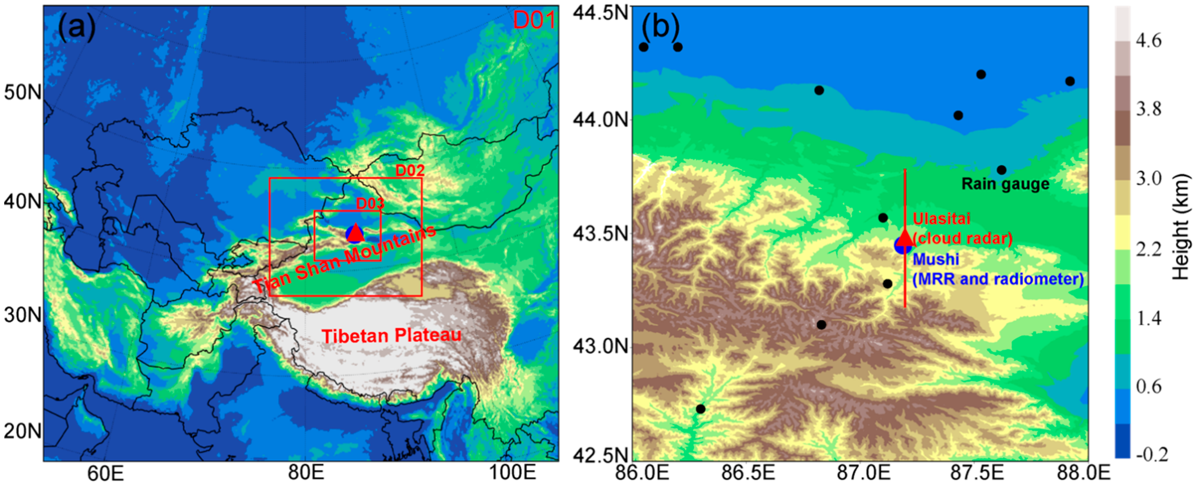
2.1. Field Measurement and Instrumentation

This field experiment was conducted over the northern slope of the middle Tian Shan area on 27 July 2019. As shown in Figure 1, a vertical pointing radiometer, located at Mushi site, was used to measure the ambient conditions such as the temperature and humidity. The precipitation rate was measured by rain gauges (Figure 1b) operated by the China Metrological Administration. Two ground-based radars, including a Ka-band cloud radar on a truck and a micro-rain radar (MRR), were deployed to measure the cloud and precipitation structure. The MRR, which has a wavelength of 12.38 mm (24 GHz), is able to measure the vertical structure of precipitation. It may respond to clouds as well if there are large particles, such as in convective clouds, but it struggles to detect cloud tops. Ka-band cloud radar is more sensitive to clouds compared to MRR because of its shorter wavelength (8.59 mm); thus, it can be used to measure the characteristics of non-precipitating clouds and for estimating the cloud tops. By combining MRR and cloud radar, the fine structure and evolution of clouds and the precipitation system could be investigated.

The radiometer had 22 channels, which were used to measure the intensity of the radiation emitted by the atmosphere from a near-surface level to a 10 km height. It included two radio frequency subsystems in the same cabinet that shared the same antenna and antenna pointing system. The temperature profiling subsystem utilized sky observations at selected frequencies between 51.25 GHz and 58 GHz. The water vapor profiling subsystem received at selected frequencies between 22.235 GHz and 28 GHz. Temperature profiles could be obtained by measuring the radiation intensity or brightness temperature using the 14 channels along the side of the oxygen feature at 60 GHz. By scanning downward from line center, where the opacity is so great that all signal originates from just above the antenna, onto the wing of the line, where the radiometer “sees” deeper into the atmosphere, the instrument could obtain altitude information. Emissions at any altitude are proportional to the local temperature and density of oxygen; thus, the temperature profile could be retrieved. Water vapor profiles could be obtained by observing the intensity and shape of emissions from pressure-broadened water vapor lines. The eight channels in the water vapor absorption band were used for the retrieval. The emissions from water vapor were in a narrow line at high altitudes and were pressure-broadened at low altitudes. The intensity of the emissions was proportional to the vapor density and temperature. Scanning the spectral profile and mathematically inverting the observed data could therefore provide water vapor profiles. The liquid water path (LWP) was obtained by measuring the contribution of vertically integrated liquid water to atmospheric spectral features of varying opacity. Liquid water information in both the oxygen and water vapor absorption bands was utilized by the radiometer. To calculate the relative contribution from liquid water, the temporally closest clear-sky opacity was used as a reference in the retrieval.

The MRR, pointing vertically with 30 range gates and a range resolution of 100 m, was located at the Mushi site (Figure 1b) and used to measure the precipitation system. The core component of the radar was a frequency-modulated Gunn diode oscillator with an integrated mixing diode. The linear polarized power was fed through a wave guide and a horn, which represented the feed of an offset paraboloid dish with a 60 cm diameter. The backscattered signal was received with the same antenna assembly. The received signal was detected by a mixing diode mounted in the wave guide between the Gunn oscillator and horn. When operated in continuous wave mode, a voltage appeared at the diode output, which depended on the phase difference between the transmit and receiving signal, and was used for further signal processing. Due to its high sensitivity and fine temporal resolution, light precipitation such as drizzle can be detected by MRR well. In the present study, the observed precipitation was light to moderate; thus, the Rayleigh approximation was applicable. The drop size distributions were retrieved based on the backscatter intensity, and the relation between terminal fall velocity and drop diameter, which was found empirically by Gunn and Kintzer [31], was put into an analytical form by Atlas [32]. The fall velocity of a rain drop is:

$$v\left(D\right)=\left(9.65-10.3·\exp \left(-0.6·D\right)\right)\delta v\left(h\right)$$

(1)

$$\delta v\left(h\right)=\left[1+3.68·{10}^{-5}h+1.71·{10}^{-9}{h}^2\right]$$

(2)

where $D$ is the drop diameter, $h$ is height, and $\delta v\left(h\right)$ is the height-dependent density correction for the fall velocity [33]. The spectral reflectivity density with respect to the drop diameter ($\eta$) can be derived using:

$$\eta \left(D,i\right)=\eta \left(v,i\right)\frac{\partial v}{\partial D}$$

(3)

where $i$ is the number of range gate. Dividing $\eta \left(D,i\right)$ by the single-particle backscattering cross-section $\sigma \left(D\right)$ yields the drop size distribution $n\left(D,i\right)$:

$$n\left(D,i\right)=\frac{\eta \left(D,i\right)}{\sigma \left(D\right)}$$

(4)

$$\sigma \left(D\right)=\frac{{\pi }^5}{{\lambda }^4}{\left|K\right|}^2{D}^6$$

(5)

$$K=\frac{m^2-1}{m^2+1}$$

(6)

where $\lambda$ is the wavelength and $m$ is the refractive index. Based on the derived drop size distributions, the drop concentration ($N$) and volume mean diameter (VMD) can be calculated using:

$$N=\underset{0}{\overset{\infty }{{\displaystyle \int }}}n\left(D\right)dD$$

(7)

$$\mathrm{VMD}={\left[\frac{{{\displaystyle \int }}_0^{\infty }n\left(D\right)D^{3}dD}{N}\right]}^{1/3}$$

(8)

In this study, we only analyze the drop size distributions, concentrations, and VMDs below the melting layer, as the existence of ice particles in the mixed-phase region may result in large uncertainties due to their complex refractive index.

The cloud radar used was a Ka-band scanning radar working at 35 GHz deployed on a truck. It generated electromagnetic waves using a solid-state transmitter and received the backscattered signal from targets such as cloud and precipitation particles. The radar could operate in either plan position indicator (PPI) or range-height indicator (RHI) mode with a beam width of 0.5°, providing measurements of reflectivity, Doppler velocity, and spectral width. During the field measurement presented in this study, the cloud radar was located at Ulasitai site, approximately 1 km north of Mushi site (Figure 1b). This was an excellent location for RHI scanning and low-elevation measurement, as it was on a relatively high hummock, with few trees surrounding it. The 0° elevation angle was unblocked to the north, west, and east, and the radar was able to detect the orographic clouds and precipitation near the surface south of the observational site. In the low-elevation measurements to the south, the return power at many radar gates was suspect because of ground clutter, the anomalous propagation of the radar beam, and other sources of interference with the terrain. However, the ground clutter could be removed because its radial velocity was always close to 0 [34]. To investigate the detailed vertical structures of orographic clouds forming due to the lifting of northerly flows forced by the Tian Shan Mountains, the radar operated on RHI scanning mode along the north–south direction, with 250 range gates and a pulse length of 150 m; thus, the maximum detection range was 37.5 km. Each RHI scan took approximately 5 min. In this study, we used the reflectivity and radial velocity obtained from the cloud radar RHI measurements. Continuous RHI measurement provided detailed information of cloud evolution.

2.2. WRF Model Setup

Radar observations can provide the fine vertical structure and temporal evolution of clouds but are insufficient for investigating the mechanisms of cloud formation and their interactions with environment. Therefore, a numerical simulation based on the WRF model was conducted to interpret the effect of the thermodynamic environment and vertical wind shear in cloud evolution. The model domain is shown in Figure 1a. The outer domain (D01) has a resolution of 9 km and the nested domain 2 (D02) has a resolution of 3 km. The inner domain (D03) has 697 × 535 grids with a resolution of 1 km and 33 stretched vertical levels topped at 50 hPa. Most of the Tian Shan Mountains are within the inner domain. The National Centers for Environmental Prediction (NCEP) Reanalysis data, which have a resolution of 0.25° × 0.25°, were used to provide the initial and boundary conditions every 6 h. The physical choices are listed in

Table 1. Configuration of the model simulation.

	D01	D02	D03
Resolution and grids	9 km, 600 × 500	3 km, 511 × 400	1 km, 697 × 535
Vertical levels	33
Cumulus	Grell–Freitas scheme	None
Microphysics	Thompson scheme
Longwave radiation	RRTMG scheme
Shortwave radiation	RRTMG scheme
Land surface	Noah scheme
Surface layer	Monin–Obukhov (Janjic Eta) scheme
PBL	MYJ scheme

. Since nested domains 2 and 3 were both convection-permitting, the cumulus scheme was turned off [6]. This configuration was established based on sensitivity tests carried out using different choices of physical schemes. The simulation ran from 6 UTC on 26 July 2019, to 18 UTC on 27 July 2019—i.e., 36 h in total; therefore, there was enough spin-up time for the convection initiation and cloud formation. The simulation was evaluated by comparing the modeled results to the radar and rain gauge measurements (see details in Section 3.2.1). In general, the model had a good performance in simulating the cloud and precipitation, and the correlation coefficient between the observed and modeled precipitation rate was as high as 0.907, providing us with the confidence to use the simulation to investigate the impact of vertical wind shear on cloud formation.

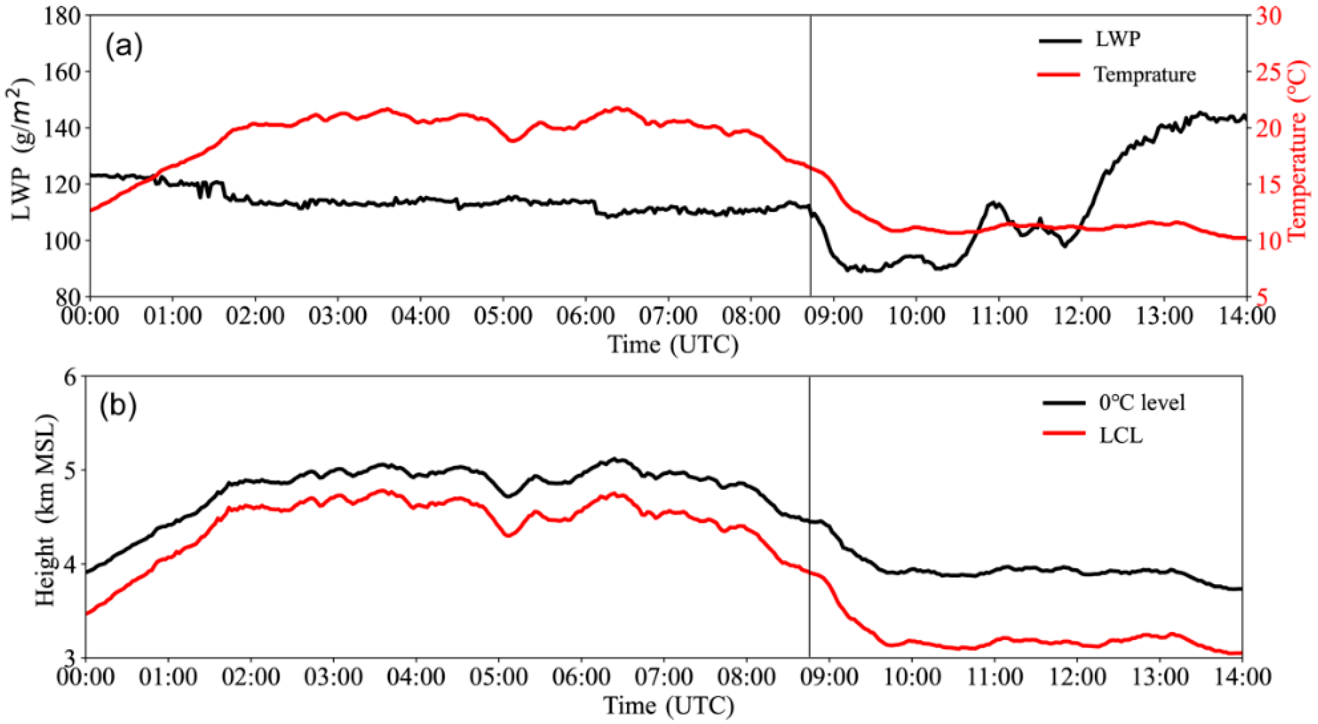
2.3. Description of the Case and Ambient Conditions

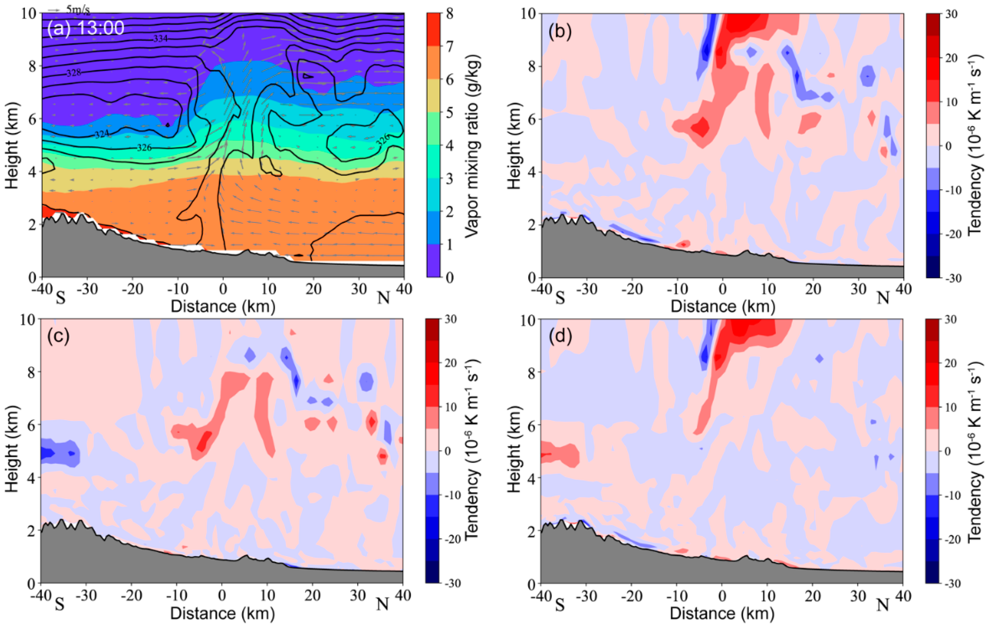
On 27 July 2019, most of the Tian Shan Mountains were covered by orographic clouds during the daytime, as can be seen from the satellite visible image at 9:00 UTC (Figure 2a). The entire storm moved west as time went on. A streamline analysis carried out at 800 hPa using the reanalysis data suggests the lifting of the flow from the opposite sides of the mountain, resulting in convergence over the mountain (Figure 2a). A sensitivity test conducted using model simulation suggests that the convergence disappeared if the sensible heat flux over the mountain was turned off (not shown), indicating the presence of anabatic winds over the Tian Shan Mountains during the daytime. This pattern can be also seen in the 700 hPa wind field (Figure 2c), which shows mainly southwesterly wind over the southern slope and northwesterly wind over the northern slope. However, it can also be seen that some wind vectors were in a southwesterly direction over the northern slope, such as near the observational site (Figure 2c), suggesting a cross-ridge flow from the southwest. This was demonstrated using the model simulation (Figure 2b), which showed that strong vertical wind shear existed at an approximately 4–5 km height. The wind was in a southwesterly or westerly direction above the wind shear level, and the low-level northwesterly wind was blocked as it reached the ridge (Figure 2b). At the upper levels (Figure 2d), the wind was westerly and controlled by a weak trough. The relative humidity at 700 hPa and 500 hPa was high over the Tian Shan Mountains, indicating a thick moisture layer, providing optimal conditions for cloud formation. Precipitation was detected by the radars in the middle of the Tian Shan area from 8:50 to 12:20 UTC (i.e., 14:50 to 18:20 local solar time) and was mostly light to moderate (weaker than 1 mm h⁻¹) in the middle of the Tian Shan area. Note that while the radar measurements can only represent clouds and precipitation within the detection range, which was small compared to the entire mountain, they are useful for investigating the fine structures of clouds.

Figure 3 shows the time series of the temperature near the surface, the LWP, the freezing level height, and the lifted condensation level (LCL) height from 0:00 to 14:00 UTC derived from the radiometer measurement. It can be seen that the temperature near surface increased from 0:00 UTC (i.e., 6:00 local solar time) and reached 23 °C at noon. The freezing level varied between 3.8 km and 5.2 km. The LCL was high before the precipitation started. After 9:00 UTC, the LCL decreased to ~3.1 km, which was close to the surface; this is because the low-level relative humidity rapidly increased (not shown) and the surface temperature rapidly decreased after the precipitation started, probably due to the evaporation of rain drops and the stronger shortwave reflection by the clouds. The LWP remained about 120 g m⁻² before the precipitation started; this was a fairly high value [35], indicating that the clouds were mostly thick. After the precipitation started, the LWP rapidly decreased, indicating a conversion from cloud to rain. After 12:20 UTC, the LWP increased again but the precipitation stopped.

To sum up, the ambient conditions were suitable for cloud formation, and convergence was generated due to the anabatic winds over the Tian Shan Mountains. Precipitation was observed over the Mushi site and Ulasitai site, and there was strong vertical wind shear at approximately 4 km. In the next section, the characteristics of the observed cloud and precipitation will be analyzed, and the role of vertical wind shear will be discussed.

3. Results

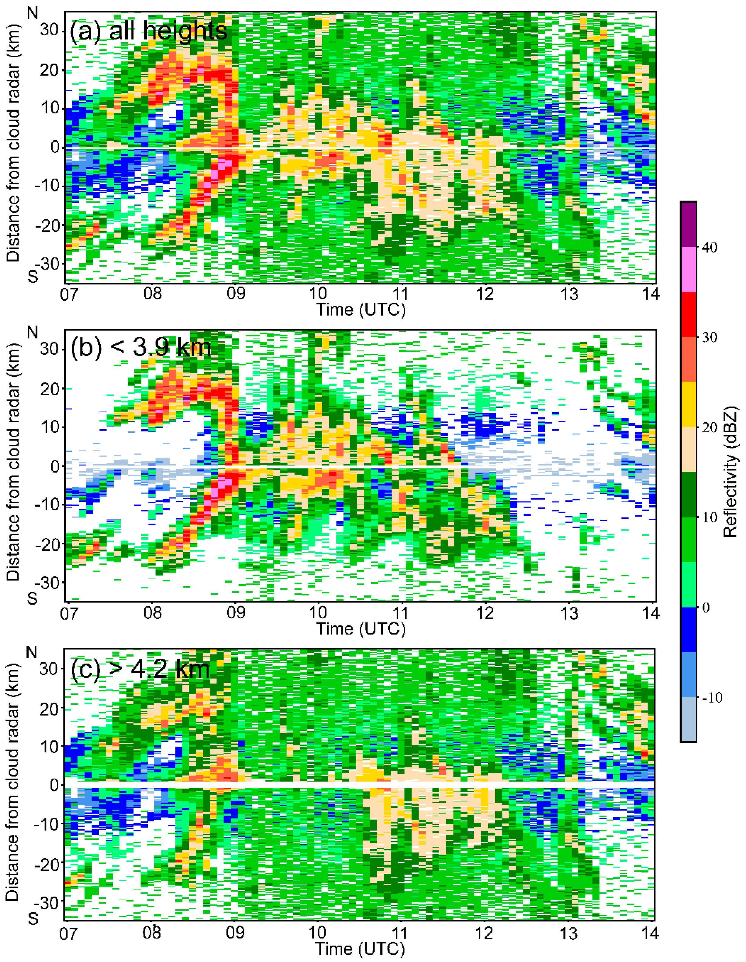
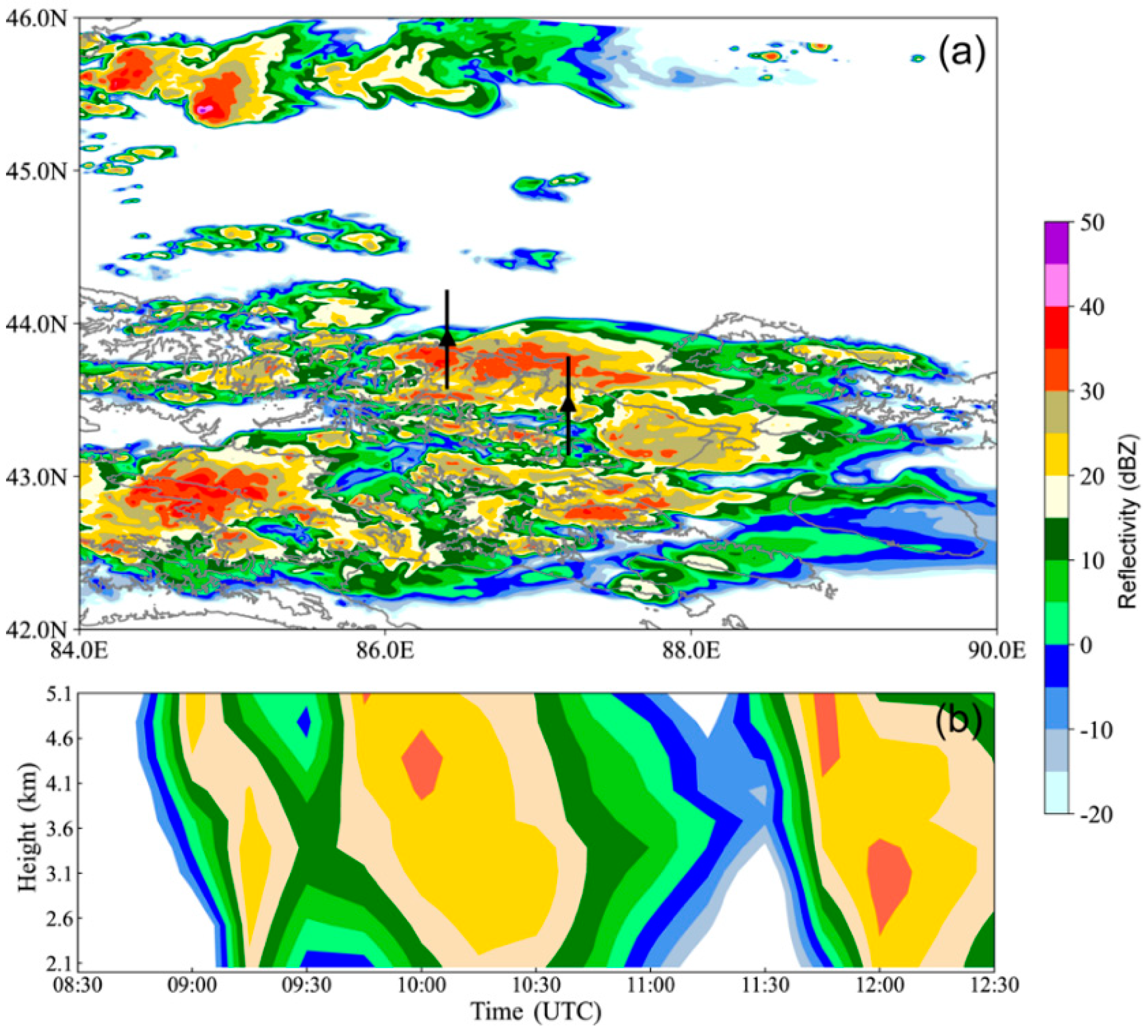
3.1. Vertical Structure and Temporal Evolution of the Orographic Clouds as Observed by Radars

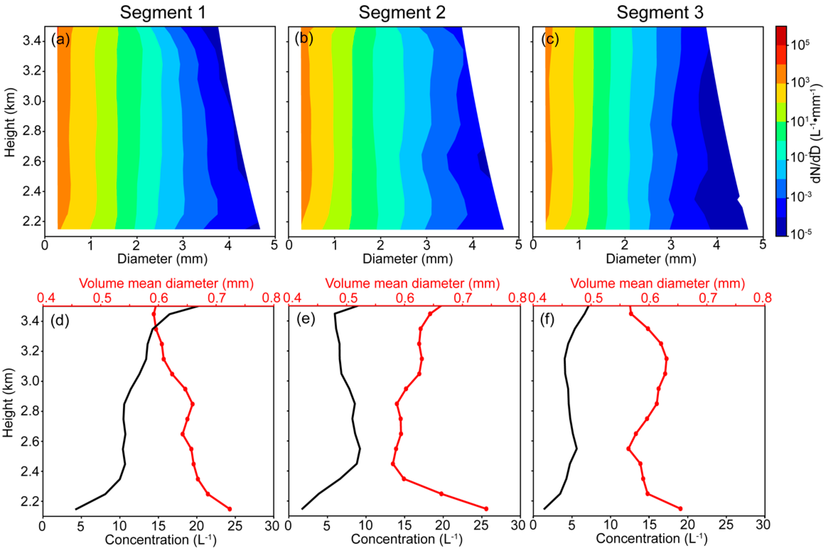
3.1.1. Characteristics of Precipitation Observed by MRR

Figure 4 shows the time–height diagrams of the reflectivity and Doppler velocity measured by the MRR. As seen from the figure, the precipitation process started at 8:50 UTC and ended at 12:20 UTC, and the MRR reflectivity near the surface ranged from approximately 10 dBZ to 30 dBZ, corresponding to a rain rate of 0.1–1 mm h⁻¹. The entire observed process can be partitioned to three segments, as indicated by the red boxes in Figure 4a. In Segment 1, precipitation quickly intensified after occurring and remained relatively strong until 9:15 UTC, then gradually weakened. In Segment 2, the low-level reflectivity was mostly around 20 dBZ, with two very short periods exceeding 25 dBZ. In Segment 3, the observational site received light and discontinuous precipitation. In all the three segments, a bright band could clearly be seen in the melting layer at about 3.7 km. The reflectivity below the melting layer was higher than that above it, partly because of the melted falling ice particles and partly because of the efficient warm rain process, as evident from cloud radar observation, which will be discussed later. The Doppler velocity was larger than 6 m s⁻¹ in the region with Z > 20 dBZ below the melting layer, indicating rain drops with an equivalent diameter of about 2 mm. Taking into account the possible updraft in the clouds, the actual terminal velocity could be larger than the measured Doppler velocity. Above the melting layer, the measured Doppler velocity was mostly 1–2 m s⁻¹, which is a typical terminal velocity of snowflakes [30]. The clear separation of the Doppler velocity above and below the melting layer indicated that the large particles in the mixed-phase region were mostly ice. However, in some regions, such as that at a 4–4.6 km height at 8:55 UTC, the Doppler velocity exceeded 4 m s⁻¹ and the reflectivity exceeded 25 dBZ, suggesting the existence of large, supercooled drops or graupels.

The drop size distributions, concentrations, and VMDs below the melting layer in the three precipitation segments are shown in Figure 5, respectively. It can be seen that the drop size distributions broadened as the rain fell toward the ground in all the segments (Figure 5a–c), indicating that the accumulation of drops was occurring, and the maximum drop diameter increased from 4 mm to approximately 4.6 mm as the rain fell from the melting layer to the surface.

The drop VMDs and concentrations had different height dependencies in the three segments. In Segment 1, the VMD generally increased (Figure 5d) and the size distribution broadened (Figure 5a) as the height decreased, indicating the continuous accumulation of rain drops. However, the evaporation and accumulation of rain drops led to a decrease in the concentration as the height decreased (Figure 5d). In Segment 2, VMD first decreased, then increased as height decreased, while the concentration varied in an opposite way (Figure 5e). This was because the evaporation of rain drops was faster than the rate of accumulation as the drops fell, and the breaking up of drops might happen; however, when approaching the surface, many small drops had fully evaporated, resulting in a broad size distribution and fewer small drops (Figure 5b); thus, the VMD was large near the surface. In Segment 3, the concentration and VMD varied similarly compared to that in Segment 2, except that, above 3.2 km, the VMD increased and the concentration decreased with the decrease in height, mainly due to the accumulation of drops.

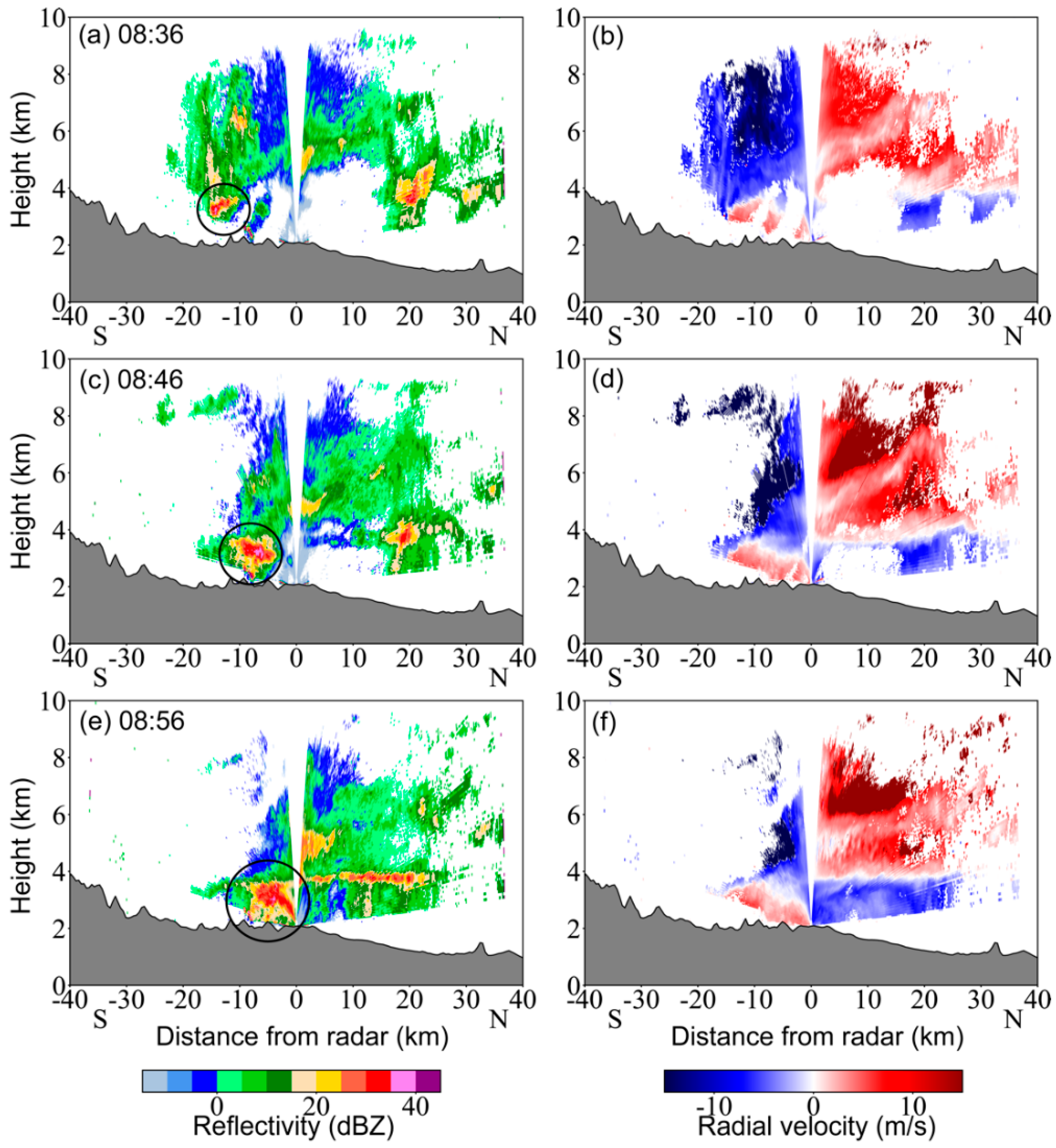
3.1.2. Characteristics of Cloud Observed by Cloud Radar

The cloud radar better shows the fine structures of the orographic clouds and precipitation; thus, it can be used to investigate the characteristics of clouds above and below the wind shear level at a height of approximately 4 km. Figure 6 shows the RHI measurements of cloud radar for Segment 1, including the reflectivity and radial velocity. The blue color of the panels of radial velocity indicates flow towards the radar, while red indicates flow away from the radar. As shown by the figure, strong wind shear existed at a height of about 4 km (Figure 6b,d,f), with a low-level northerly upslope wind and higher-level cross-ridge southwesterly wind; this confirms the wind field modeled by WRF (Figure 2b). The cloud top height was approximately 9 km, corresponding to a cloud top temperature of −30 °C. It can be seen that the cloud structure was very different above and below the wind shear level. Below 4 km, a convective cell was formed at 8:36 UTC to the south of the radar, along the boundary of the cross-ridge southwesterly flow and the upslope northerly flow. The cell intensified as it moved gradually to the north (shown by the black circles in Figure 6a,c,e). At 8:46 UTC, light precipitation occurred below the convective cell, and the precipitation intensified as the cell matured. An important aspect to note was that the cell top rarely exceeded the wind shear level. The clear separation between the cell and upper-level clouds suggests that the precipitation was mainly due to warm rain rather than mixed-phase cloud. Falling ice did occur, as seen from the bright band on the north side of the radar at about 3.8 km at 8:56 UTC (Figure 6e), but the rainfall from the melted snow was much weaker than the warm rain generated by the convective cell. The convective cell dissipated after 9:10 UTC (not shown), meaning that the observed precipitation was weakened (Figure 4a).

Figure 7 shows the RHI measurements from the cloud radar for Segment 2. The cloud structures remained different above and below the shear level. The radar echo was mostly weak above 4 km, indicating non-precipitating clouds, although ice particles might exist in regions with a reflectivity exceeding 10 dBZ. Below the wind shear level, the warm rain process was still efficient, generating light to moderate precipitation (Figure 4). The radar reflectivity was relatively high (>20 dBZ) in the convergence regions, such as that 10 km north of the radar at a ~3 km height in Figure 7a,b. At 10:32 UTC, the wind field changed, as can be seen from the radial velocity measured by the cloud radar (Figure 7f); the wind near the surface turned to the south; between 3 km and 4 km, the wind was still northerly; and above 4 km, the wind was southerly. Therefore, two vertical wind shear levels were present. This limited most of the warm clouds between 3 km and 4 km at 10:32 UTC, as seen from the radar echoes (Figure 7e); the reflectivity was 5–20 dBZ within the cloud, but low both near the surface and above the shear level.

In Segment 3 (Figure 8), the wind field became more complicated. At 11:17 UTC, the reflectivity was mostly weak, except a few isolated echoes exceeding 20 dBZ, associated with weak convergence zones. At 11:47 UTC, there were two clear vertical wind shear levels, as shown in Figure 8d, which resulted in multiple layers of clouds. The highest layer of cloud, observed above the higher level of wind shear (Figure 8c), formed because the moist cross-ridge flow was lifted by the lower dry northerly flow (Figure 8d) and was possibly related to the lee wave of the cross-ridge flow as well; however, this cannot be verified using radar data alone. The cloud base had a similar shape compared to the structure of the vertical wind shear. At 3.5 km, a thin cloud layer formed along the lower wind shear level and the shape of the cloud top was consistent with the lower southerly flow, again revealing the importance of the vertical wind shear for the cloud formation and evolution. There was a third layer of cloud near the surface, with a few weak cells generated due to local convergence. The upper two cloud layers were mostly decoupled from the surface, and the precipitation was mainly generated by the warm rain process. This pattern continued (Figure 8e,f) until the cloud dissipated and the rain stopped (Figure 4). The warm cloud rarely exceeded the vertical wind shear level above its top, suggesting an inhibiting impact on the cloud vertical development.

The temporal evolution of clouds can be described using the time series of the composite reflectivity (i.e., the maximum reflectivity in each vertical column) along the RHI cross-section. Figure 9a is the composite reflectivity for all heights, and Figure 9b,c are for the heights below 3.9 km and above 4.2 km, which represent the clouds below and above the vertical wind shear level. It can be seen from the figure that that cloud evolution was very different above and below the wind shear level. Between 7:00 and 9:40 UTC (corresponding to the first precipitation segment), the temporal variation in precipitation (Figure 9a) was controlled by the warm rain process below the wind shear level (Figure 9b) and the maximum reflectivity was approximately 35 dBZ. The observed clouds moved northwards. Scattered non-precipitating warm clouds and upper-level clouds were observed before 8:00 UTC. Two convective cells were generated at about 8:00 UTC and produced warm rain at the observational site from 8:50 to 9:40 UTC. The second precipitation segment (9:45–10:40 UTC) was dominated by a warm rain process as well. Clouds were rarely seen above the wind shear level (Figure 9c), suggesting the presence of a dry cross-ridge southwesterly flow and a lack of strong convection. The composite reflectivity was much lower than that in Segment 1, indicating a weaker warm rain process. In Segment 3 (10:55–12:10 UTC), clouds both above and below the wind shear level contributed to the overall composite reflectivity. The low-level clouds contributed relatively more to the echoes stronger than 30 dBZ, but they were more scattered and short-lived. The clouds covered similar areas above and below the vertical wind shear level, but the clouds were more homogeneous above the wind shear level, while clouds below the shear level had a higher variability. We can see from Figure 9 that the precipitation processes were quite different in the three segments. Although all the clouds in the three segments were related to the anabatic winds over the Tian Shan Mountains, the ambient conditions changed significantly with time, since the prevailing wind was westerly in this case. Therefore, the different cloud formation mechanisms led to various characteristics of precipitation in the three segments.

To sum up, we can see that based on the radar observations, the clouds had very different structures and temporal evolutions above and below the wind shear level, indicating the vertical wind shear had an important impact on the cloud development. First of all, the top of the convective cells generated near the surface rarely exceeded the wind shear level; thus, the precipitation was mostly warm rain, suggesting that vertical wind shear had an inhibiting impact on the vertical development of convection. In addition, multiple layers of clouds were generated, and their shapes were consistent with the structure of vertical wind shear; thus, their formation was strongly related to the vertical wind shear. Moreover, the cloud evolution and precipitation were strongly controlled by the combination of convective instability and vertical wind shear. The different thermodynamic and shear conditions resulted in significant differences in the three segments of the precipitation process. The analysis shown above reveals the advantages of using millimeter radars for measuring the fine structures of orographic clouds over the Tian Shan Mountains under ambient conditions with a strong vertical wind shear. However, the mechanisms of vertical wind shear influencing the cloud development cannot be fully understood using observations alone, so the result from a convection-permitting resolution simulation is analyzed in the next section.

3.2. Impact of Vertical Wind Shear on Clouds as Interpreted from Model Simulation

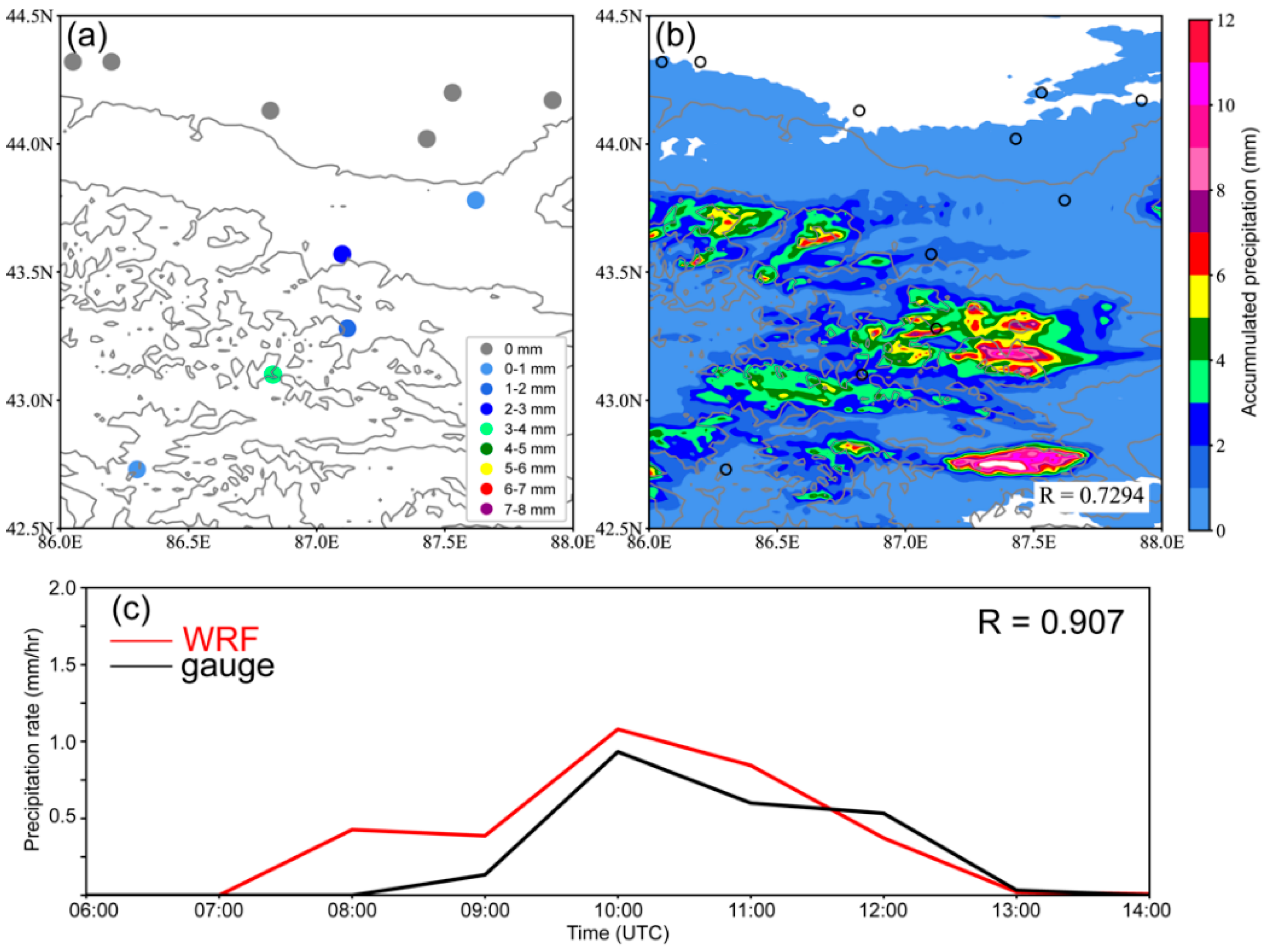
3.2.1. Model Evaluation

Before analyzing the simulated results, the modeled clouds and precipitation need to be evaluated. Figure 10 shows the map of composite reflectivity in the inner domain modeled by WRF and the time–height diagram of the modeled reflectivity. The distribution of composite reflectivity can be evaluated using Figure 2a, though this is not a direct comparison. It can be seen that WRF can capture the general distribution of orographic cloud and precipitation well compared to satellite images (Figure 10a). Most of the Tian Shan Mountains were covered by orographic clouds in this case, and precipitation was detected over both slopes. The maximum modeled radar reflectivity was found to be about 35 dBZ, and the modeled echoes with a high reflectivity revealed that convection was occurring over the mountain. Note that we are not focusing on large-scale precipitation in this paper, but rather the consistency between the modeled and observed cloud distributions is the basis for our analysis of the detailed cloud evolution using model outputs. To evaluate the cloud evolution more directly, we plot the modeled radar reflectivity in Figure 10b, which can be compared to the MRR reflectivity shown in Figure 4a. As seen from the figure, WRF captured the temporal evolution of the clouds well. Precipitation started at approximately 9:00 UTC, and there were three segments of precipitation. However, due to the relatively low resolution, the fine structures of the clouds cannot be represented.

The precipitation modeled using WRF is evaluated in Figure 11. In the central Tian Shan area, the accumulated precipitation from the WRF model (Figure 11b) was consistent with that measured by the rain gauges (Figure 11a). The correlation coefficient between the model and the observation was greater than 0.7. In addition, WRF showed that relatively more precipitation was received over the ridges and less at the foot of the mountains. Near the observational site, the amount of accumulated precipitation was 3–7 mm in this case. The average observed precipitation rate of the three gauges on the north slope of the central Tian Shan area varied between 0 and 1 mm h⁻¹ (Figure 11c). The precipitation rate modeled at these three stations was slightly larger than the observed rate, and the precipitation started slightly earlier. However, the variations in the precipitation rate seen between the model and observation were consistent, with a correlation coefficient of 0.907. Sensitivity tests conducted using several other configurations of WRF provided worse results for the modeled cloud and precipitation (not shown).

In general, WRF captured the characteristics of the cloud evolution and precipitation reasonably well. However, there were some differences between the modeled and observed precipitation structures for multiple reasons. Firstly, the model resolution was 1 km, much larger than the resolution of MRR, and the vertical structure of the precipitation was not as fine as that in the MRR observation. In addition, a 1 km resolution cannot fully reveal the terrain complexity, which may have an important impact on the small-scale structure of orographic precipitation. Moreover, the reflectivity modeled from the WRF output was for a radar wavelength of 10 cm, which was different than the MRR wavelength; thus, the magnitudes of reflectivity were expected to differ between the model and the observation. Finally, there were many sources of uncertainty in modeling orographic clouds using the WRF, especially in the boundary layer and the microphysics parameterizations [5]. In this study, the modeled results were mainly used to investigate the thermodynamic conditions and the impact of vertical wind shear (Section 3.2.2); the 1 km resolution simulation was sufficient for this goal, and the modeled results were reasonably good for analyzing the temporal evolution of clouds. For the simulation of the fine structures of clouds and the impact of small-scale orographic features, a large eddy simulation is necessary and will be conducted in the future.

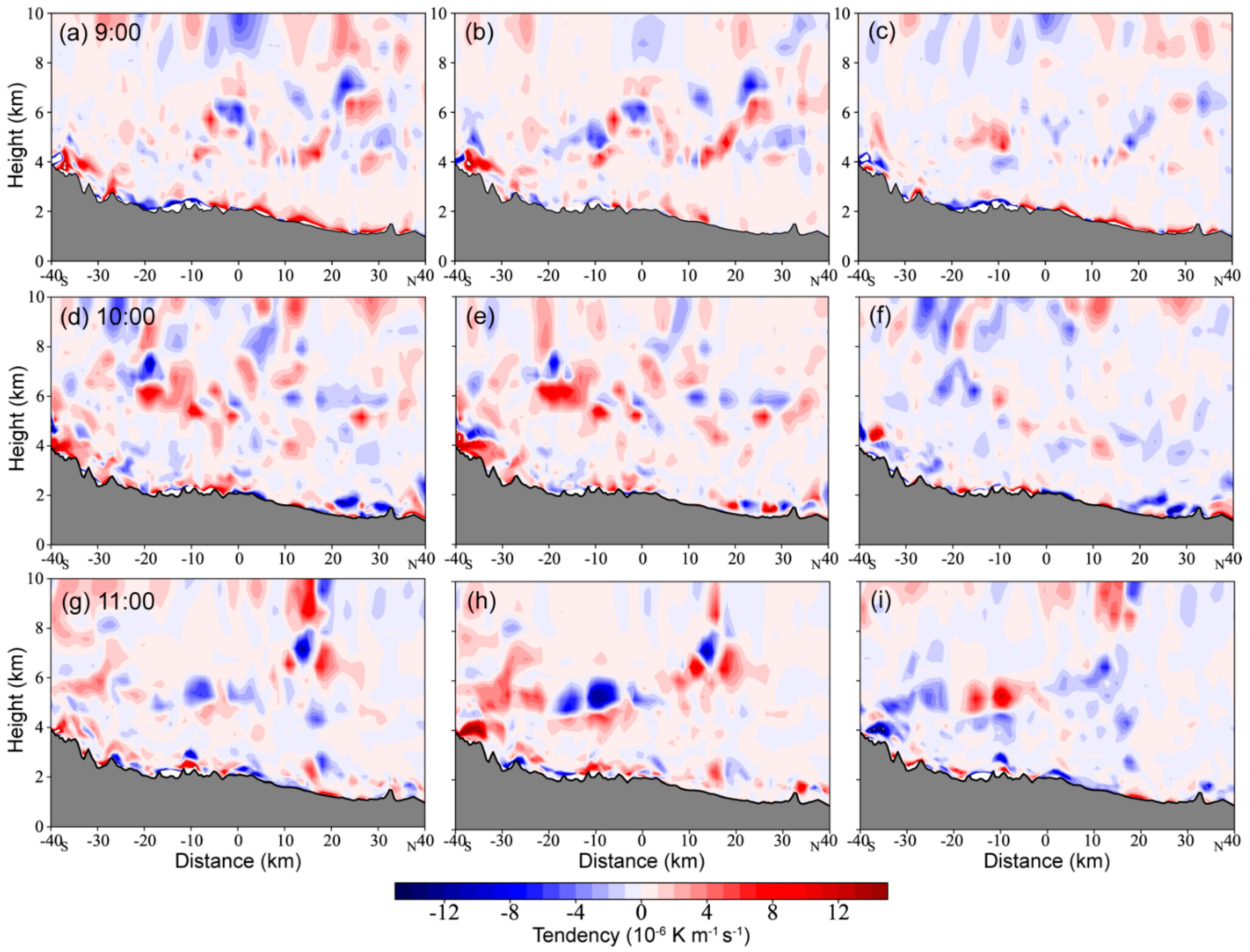
3.2.2. The Impact of Vertical Wind Shear on Clouds

Figure 12 shows the modeled cross-section of equivalent potential temperature, wind vectors, and water vapor mixing ratio along the east black line (same as the RHI scan of cloud radar shown in Figure 10a). At 8:00 UTC, low-level convective instability was present, as seen from the decrease in potential temperatures with height in some areas, such as 30 km south of the radar, and we can see there was updraft due to the convergence between the cross-ridge flow and the northerly upslope wind. The vapor mixing ratio was high in the convergence zone, providing favorable conditions for convective cloud formation. The updraft was weakened at 8:30 UTC, and the convergence zone moved northward (Figure 12b,c), consistent with the cloud radar observation. Strong vertical wind shear persisted at approximately 4–5 km during this case, and most of the time, the convection was limited to beneath the shear level. The low-level humidity kept increasing during the precipitation process (Figure 12a–f), probably due to the evaporation of rain drops, while the upper-level humidity showed no significant change. The small-scale gravity waves forced by the terrain provided weak updrafts near the surface and were responsible for the generation of weak convergences, which contributed to the formation of low-level warm clouds.

Another feature seen from the figure is that lee waves from the southernly cross-ridge flow were present. For example, at 10:00 and 11:00 UTC, there were clear lee waves at heights of about 5–6 km above the observational site, generating updraft and downdraft (Figure 12e,f). Below the lee waves, a weak northernly flow was found, forming vertical wind shear. This explains the formation of the observed stratiform clouds at this level (Figure 7a and Figure 8c). The wind near the surface at 11:00 UTC turned to a southerly direction; thus, two wind shear levels were present, consistent with radar observation. Convective instability still can be seen near surface, and the high relative humidity provided good conditions for forming low-level warm clouds, but no strong updraft was seen at 11:00 UTC; thus, the precipitation seen in Segment 3 was determined to be light.

To investigate the impact of vertical wind shear on the convection, we analyzed the tendency of the convective stability, which can be expressed using:

$$\frac{d}{dt}\left(\frac{\partial {\theta }_e}{\partial z}\right)=m_1+m_2$$

(9)

$$m_1=-\frac{\partial u}{\partial z}\frac{\partial {\theta }_e}{\partial x}-\frac{\partial v}{\partial z}\frac{\partial {\theta }_e}{\partial y}$$

(10)

$$m_2=\left(\frac{\partial u}{\partial x}+\frac{\partial v}{\partial y}\right)\frac{\partial {\theta }_e}{\partial z}$$

(11)

where $m_1$ is the vertical wind shear term and $m_2$ is the divergence term. Positive values of $m_1$ and $m_2$ result in an enhancement in convective stability, while negative values of $m_1$ and $m_2$ indicate a decline in convective stability (i.e., a more unstable atmosphere) due to the vertical wind shear and divergence. Figure 13 shows the convective stability, the vertical wind shear term, and the divergence term of the convective stability tendency modeled by WRF at 9:00, 10:00, and 11:00 UTC, respectively. It can be seen from the figure that the tendency of convective stability was highly variable because of the high spatial variability of the potential temperature (Figure 12c). The overall tendency (left panels) was dominated by the vertical wind shear term (middle panels) at most of the heights, and impacted by both the vertical wind shear and divergence term near the surface. The main point here is that below the vertical wind shear level, the tendency of convective stability was mostly positive (Figure 13a,b,d,e,g,h), preventing the low-level convection from persisting. Although convective updrafts were found (Figure 12c), they could hardly exceed the vertical wind shear level. Above 5 km, the tendency of convective stability was negative in some areas, which was related to the lee waves. However, since the atmosphere was mostly stable above 5 km, no elevated convection was observed. The divergence term was mostly negative below the vertical wind shear level, which had a positive impact on the convection formation and persistence. However, the magnitude of the convergence was weak (Figure 13c,f,i); thus, it was not able to dominate the tendency of convective stability. In general, based on the tendency analysis of convective stability, we can see the vertical wind shear had an inhibiting impact on the convective stability, and though low-level convergence was present and updrafts were generated in some areas (Figure 12), the convections were limited beneath the shear level and were barely present during the precipitation process.

4. Discussion

The analysis shown above indicates that millimeter radar is a powerful tool with which to study the fine structure of orographic clouds and precipitation because of its high temporal and spatial resolution. In this case, the vertically pointing K-band MRR presented the temporal evolution of precipitation and the differences in rain microphysics during different precipitation segments well. The Ka-band cloud radar also showed the fine structures of clouds in an ambient condition with vertical wind shear well. The measurements clearly indicated that the cloud formation and evolution were strongly controlled by the vertical wind shear based on the reflectivity and radial velocity. A combination of millimeter radar measurements and high-resolution simulation effectively revealed the role of vertical wind shear in the process of cloud development, including the inhibitive impact of the vertical wind shear on the development of convective cells and the formation of multi-layer clouds.

However, one limitation of millimeter radar measurement is its relatively small detection range; thus, the results shown in this paper are only relevant for the clouds in the sample area. It can be seen from the satellite measurement (Figure 2a) and model simulation (Figure 10a) that the clouds covered the entire area of the Tian Shan Mountains in this case and the spatial variability was large, suggesting that the clouds that formed at different locations had different characteristics. Therefore, clouds formed outside of the radar detection range might interact with vertical wind shear differently. For example, Figure 14 shows the thermodynamic conditions along the west black line shown in Figure 10, where a deeper level of convection occurred. The vertical wind shear at ~4 km was weak, and the convergence induced between the southerly and northerly flow was strong (Figure 14a). As the vertical wind shear was balanced by the upslope wind, continuous convection could be triggered. Thus, the convection was as deep as 9 km and the vertical velocity was nearly 15 m s⁻¹. The tendency of convective stability (Figure 14b) was influenced by both the vertical wind shear and divergence in similar magnitudes, and both of them had a negative impact on the stability below 4 km (Figure 14c,d). The divergence was strong above 9 km due to the stable atmosphere (Figure 14a,d), preventing the upward development of convection. A previous study conducted using the WRF model also indicated that deep convective clouds may form over the Tian Shan Mountains despite the presence of strong vertical wind shear [10].

The impact of vertical wind shear on cloud development over the Tian Shan Mountains could be more complicated than that over a plain. Firstly, the convective precipitation had a diurnal variation over the Tian Shan Mountains. Li et al. [36] showed that during summer, the peak precipitation rate was found over the mountain ridge in the late afternoon and moved northward as time went on. Therefore, the heights of the vertical wind shear level relative to the convection initiated near the surface may vary diurnally. For wind shear close to the surface, an inhibiting impact on the convection initiation could be expected if the shear was strong enough, while if the shear was well above the surface, convective clouds could develop to a higher level, thus interacting with vertical wind shear in a different way. Additionally, the vertical wind shear was often influenced by gravity waves induced by the Tian Shan Mountains. An example of this is the lee wave of the southerly cross-ridge flow. A strong updraft or downdraft in a gravity wave could affect the cloud dynamics, organization, and microphysics, leading to a complicated interaction occurring among clouds, gravity waves, and vertical wind shear. Moreover, Tian Shan Mountains are a large system consisting of ranges and valleys, so small-scale orographic features may have important impacts on the interaction between the ambient environment and clouds [37,38]. For example, over plains, convection could be intensified if strong low-level vertical wind shear was balanced by a gust front, while over mountains, this balance may be destroyed by the local dynamics induced by small-scale topography. Till now, most of the previous studies on this topic focused on clouds over plains, and the present study only focuses on a single case. Therefore, in order to better understand the impact of vertical wind shear on cloud formation over mountains, more observational and modeling studies need to be carried out in the future.

5. Conclusions

In this research, a case study was conducted to investigate the impact of vertical wind shear on the summer orographic cloud and precipitation over the Tian Shan Mountains. Multiple remote sensors were deployed in the field experiment, including a radiometer to measure the ambient conditions, a vertically pointing micro-rain radar to measure the vertical structure and temporal evolution of the precipitation, and a Ka-band cloud radar to detect the fine structures of the orographic clouds. In addition, a convection-permitting simulation was conducted to investigate the role of vertical wind shear. Our main findings are as follows:

(1)

The MRR measurements show that the case presented in this paper had three segments of precipitation. The precipitation was light to moderate and no strong convection occurred. The precipitation was mainly due to the warm rain process, though snowflakes fell in the mixed-phase region. In all three segments, the drops size distributions broadened as the rain fell towards the surface, but the concentrations and VMDs varied differently with height, depending on the rate of evaporation and the accumulation of rain drops.

(2)

The cloud radar measurements show that the clouds had very different structures and temporal evolutions above and below the vertical wind shear level, indicating that vertical wind shear had an important impact on the cloud development. Firstly, the top of the convective cells rarely exceeded the wind shear level, suggesting that the vertical wind shear had an inhibiting impact on the development of convection. Additionally, the formation of multiple layers of clouds was strongly related to the vertical wind shear, since their shapes were consistent with the structure of vertical wind shear. Moreover, the different thermodynamic and shear conditions resulted in significant differences in the three segments of the precipitation process.

(3)

The results obtained from the WRF model indicate that low-level convective instability existed on the north slope of the mountain, providing favorable conditions for convection formation near the surface. However, the tendency analysis suggested that the vertical wind shear dominated the variation in convective stability and had a negative effect on the convection below the wind shear level. This explains why the convective clouds were short-lived and rarely exceeded the shear level, and confirms that the vertical wind shear had an inhibiting impact on the vertical development of clouds.

The analysis shown in this study highlights the advantages of using millimeter radars for measuring the fine structures of orographic clouds over complex terrain; thus, they can be used to study the interactions between the vertical wind shear and cloud development. The findings show that the vertical wind shear not only influences the development of convection but also has an impact on the formation of multi-layer clouds over mountains, as it may interact with gravity waves. Therefore, it is necessary to consider the role of complex terrain when analyzing the interaction between vertical wind shear and clouds over mountains. The main limitations of millimeter radar are its relatively small sample area and the blockage of low-elevation beams by ground clutter. The use of a combination of large eddy simulation, ground-based radar observation, and aircraft measurements will help us to better understand the orographic clouds and precipitation over complex terrain in the future, including aspects such as the impact of shear-induced turbulence on clouds; the impact of vertical wind shear on cloud microphysics, and the interactions among vertical wind shear, small-scale orographic features, and clouds.

References

1. Ma, S.; Xi, Y. Some regularities of storm rainfall in Xinjiang, China. Acta Meteorol. Sin. 1997, 55, 239–248. (In Chinese) [Google Scholar]
2. Shi, Y.; Sun, Z.; Yang, Q. Characteristics of area precipitation in Xinjiang region with its variations. J. Appl. Meteorol. Sci. 2008, 19, 326–332. (In Chinese) [Google Scholar]
3. Zhao, C.; Ding, Y.; Ye, B.; Zhao, Q. Spatial distribution of precipitation in Tian Shan Mountains and its estimation. J. Adv. Water Sci. 2011, 22, 315–322. (In Chinese) [Google Scholar]
4. Zhang, Z.; He, X.; Liu, L.; Li, Z.; Wang, P. Spatial distribution of rainfall simulation and the cause analysis in China’s Tian Shan Mountains area. Adv. Water Sci. 2015, 26, 500–508. (In Chinese) [Google Scholar]
5. Liu, C.; Ikeda, K.; Thompson, G.; Rasmussen, R.; Dudhia, J. High-resolution simulations of wintertime precipitation in the Colorado Headwaters region: Sensitivity to physics parameterizations. Mon. Weather Rev. 2011, 139, 3533–3553. [Google Scholar] [CrossRef]
6. Jing, X.; Geerts, B.; Wang, Y.; Liu, C. Evaluating Seasonal Orographic Precipitation in the Interior Western United States using Gauge Data, Gridded Precipitation Estimates, and a Regional Climate Simulation. J. Hydrometeorol. 2017, 18, 2541–2558. [Google Scholar] [CrossRef]
7. Yang, L. Research on a Case of Heavy Rain in Xingjiang from South Asia High Abnormity. Meteorol. Mon. 2003, 29, 21–25. (In Chinese) [Google Scholar]
8. Wang, X.; Xu, X.; Wang, W. Characteristic of Spatial Transportation of Water Vapor for Northwest China′s Rainfall in Spring and Summer. Plateau Meteorol. 2007, 16, 52–62. (In Chinese) [Google Scholar]
9. Yao, J.; Yang, Q.; Huang, J.; Zhao, L. Computation and Analysis of Water Vapor Content in Tian Shan Mountains and Peripheral Regions, China. Arid Zone Res. 2012, 29, 567–573. (In Chinese) [Google Scholar]
10. Lian, Y.; Yang, J.; Zhu, L.L. A numerical study of the severe convective precipitation processes over the middle section of the eastern Tian Shan Mountains during the summer seasons. Trans. Atmos. Sci. 2017, 40, 663–674. (In Chinese) [Google Scholar]
11. Huang, X.; Zhou, Y.; Ran, L.; Kalim, U.; Zeng, Y. Analysis of the Environmental Field and Unstable Conditions on A Rainstorm Event in the Ili Valley of Xinjiang. Chin. J. Atmos. Sci. 2021, 45, 148–164. (In Chinese) [Google Scholar]
12. Chen, T. The Characteristics of Hourly Precipitation in Tian Shan Mountain during Summer. Master’s Thesis, Chinese Academy of Meteorological Sciences, Beijing, China, 2017; p. 67. (In Chinese). [Google Scholar]
13. Jiang, C.; Guo, Q.; Li, J.; Li, Y. A Preliminary Analysis of Formational Causes of a Heavy Rain in North Slope of Tian Shan Mountains. J. Arid. Land Resour. Environ. 2013, 27, 160–166. (In Chinese) [Google Scholar]
14. Richardson, Y.P.; Droegemeier, K.K.; Davies-Jones, R.P. The influence of horizontal environmental variability on numerically simulated convective storms. Part I: Variations in vertical shear. Mon. Weather Rev. 2007, 135, 3429–3455. [Google Scholar] [CrossRef] [Green Version]
15. Markowoski, P.; Richardson, Y. Mesoscale Meteorology in Midlatitudes; Wiley-Blackwell: Hoboken, NJ, USA, 2012; p. 407. [Google Scholar]
16. Chen, Q.; Fan, J.; Hagos, S.; Gustafson, W.I., Jr.; Berg, L.K. Roles of wind shear at different vertical levels: Cloud system organization and properties. J. Geophys. Res. Atmos. 2015, 120, 6551–6574. [Google Scholar] [CrossRef]
17. Lasher-Trapp, S.; Kumar, S.; Moser, D.H.; Blyth, A.M.; French, J.R.; Jackson, R.C.; Leon, D.C.; Plummer, D.M. On Different Microphysical Pathways to Convective Rainfall. J. Appl. Meteorol. Climatol. 2018, 57, 2399–2417. [Google Scholar] [CrossRef]
18. Helfer, K.C.; Nuijens, L.; de Roode, S.R.; Siebesma, A.P. How Wind Shear Affects Trade-wind Cumulus Convection. J. Adv. Model. Earth Syst. 2020, 12, e2020MS002183. [Google Scholar] [CrossRef]
19. Rotunno, R.; Klemp, J.B.; Weisman, M.L. A theory for strong, long-lived squall lines. J. Atmos. Sci. 1988, 45, 463–485. [Google Scholar] [CrossRef] [Green Version]
20. Weisman, M.L.; Rotunno, R. “A theory for strong long-lived squall lines” revisited. J. Atmos. Sci. 2004, 61, 361–382. [Google Scholar] [CrossRef]
21. DeLonge, M.S.; Fuentes, J.D.; Chan, S.; Kucera, P.A.; Joseph, E.; Gaye, A.T.; Daouda, B. Attributes of mesoscale convective systems at the land-ocean transition in Senegal during NASA African Monsoon Multidisciplinary Analyses 2006. J. Geophys. Res. Atmos. 2010, 115, D10213. [Google Scholar] [CrossRef] [Green Version]
22. Coniglio, M.C.; Stensrud, D.J.; Wicker, L.J. Effects of upper-level shear on the structure and maintenance of strong quasi-linear mesoscale convective systems. J. Atmos. Sci. 2006, 63, 1231–1252. [Google Scholar] [CrossRef] [Green Version]
23. Wang, C.; Prinn, R.G. Impact of the horizontal wind profile on the convective transport of chemical species. J. Geophys. Res. Atmos. 1998, 103, 22063–22071. [Google Scholar] [CrossRef]
24. Sathiyamoorthy, V.; Pal, P.K.; Joshi, P.C. Influence of the upper-tropospheric wind shear upon cloud radiative forcing in the Asian monsoon region. J. Clim. 2004, 17, 2725–2735. [Google Scholar] [CrossRef]
25. Fan, J.; Yuan, T.; Comstock, J.M.; Ghan, S.; Khain, A.; Leung, L.R.; Li, Z.; Martins, V.J.; Ovchinnikov, M. Dominant role by vertical wind shear in regulating aerosol effects on deep convective clouds. J. Geophys. Res. 2009, 114, D22206. [Google Scholar] [CrossRef]
26. Chen, Q.; Fan, J.; Yin, Y.; Han, B. Aerosol impacts on mesoscale convective systems forming under different vertical wind shear conditions. J. Geophys. Res. Atmos. 2020, 125, e2018JD030027. [Google Scholar] [CrossRef]
27. Yang, J.; Wang, Z.; Heymsfield, A.J.; French, J.R. Characteristics of Vertical Air Motion in Isolated Convective Clouds. Atmos. Chem. Phys. 2016, 16, 10159–10173. [Google Scholar] [CrossRef] [Green Version]
28. Wang, Z.; French, J.; Vali, G.; Wechsler, P.; Haimov, S.; Rodi, A.; Deng, M.; Leon, D.; Snider, J.; Peng, L.; et al. Single aircraft integration of remote sensing and in situ sampling for the study of cloud micro-physics and dynamics. Bull. Amer. Meteor. Soc. 2012, 93, 653–668. [Google Scholar] [CrossRef] [Green Version]
29. Jing, X.; Geerts, B. Dual-Polarization Radar Data Analysis of the Impact of Ground-Based Glaciogenic Seeding on Winter Orographic Clouds. Part II: Convective Clouds. J. Appl. Meteor. Climatol. 2015, 54, 2099–2117. [Google Scholar] [CrossRef]
30. Geerts, B.; Yang, Y.; Rasmussen, R.; Haimov, S.; Pokharel, B. Snow Growth and Transport Patterns in Orographic Storms as Estimated from Airborne Vertical-Plane Dual-Doppler Radar Data. Mon. Weather. Rev. 2015, 143, 644–665. [Google Scholar] [CrossRef] [Green Version]
31. Gunn, R.; Kintzer, G. The terminal velocity of fall for water droplets in stagnant air. J. Meteor. 1949, 6, 243–248. [Google Scholar] [CrossRef] [Green Version]
32. Atlas, D.; Srivastava, R.; Sekhon, R. Doppler radar characteristics of precipitation at vertical incidence. Rev. Geophys. 1973, 11, 1–35. [Google Scholar] [CrossRef]
33. Foote, G.B.; du Toit, P.S. Terminal velocity of raindrops aloft. J. Appl. Meteorol. 1969, 8, 249–253. [Google Scholar] [CrossRef] [Green Version]
34. Gourley, J.J.; Tabary, P.; Du Chatelet, J.P. A fuzzy logic algorithm for the separation of precipitating from nonprecipitating echoes using polarimetric radar observations. J. Atmos. Ocean. Technol. 2007, 24, 1439–1451. [Google Scholar] [CrossRef]
35. O’Dell, C.W.; Wentz, F.J.; Bennartz, R. Cloud Liquid Water Path from Satellite-Based Passive Microwave Observations: A New Climatology over the Global Oceans. J. Clim. 2008, 21, 1721–1739. [Google Scholar] [CrossRef]
36. Li, J.; Chen, T.; Li, N. Diurnal Variation of Summer Precipitation across the Central Tian Shan Mountains. J. Appl. Meteorol. Climatol. 2017, 56, 1537–1550. [Google Scholar] [CrossRef]
37. Cosma, S.; Richard, E.; Miniscloux, F. The role of small-scale orographic features in the spatial distribution of precipitation. Q. J. R. Meteorol. Soc. 2002, 128, 75–92. [Google Scholar] [CrossRef]
38. Kirshbaum, D.J.; Durran, D.R. Observations and modeling of banded orographic convection. J. Atmos. Sci. 2005, 62, 1463–1479. [Google Scholar] [CrossRef]
Figure 1. (a) Domains of the WRF model simulation and topography. D01, D02, and D03 indicate the three nested domains used in the simulation; (b) Topography of the middle of the Tian Shan area. The red triangle indicates the location of Ka-band radar, the red vertical line in (b) indicates the range of the range–height indicator (RHI) scan, the blue dot indicates the location of an MRR, and the black dots in (b) indicate the locations of rain gauges.
Remotesensing 14 01583 g001
Figure 2. (a) Visible image observed from the FY4A satellite and streamlines at 800 hPa; (b) Cross–section of wind vectors along the red line shown in (a); (c,d) Geopotential height (black lines), wind barbs, and relative humidity (colored) at 700 hPa and 500 hPa at 9:00 UTC on 27 July 2019. S and N below (b) indicate south and north of the cloud radar.
Remotesensing 14 01583 g002
Figure 3. Time series of (a) temperature near surface (red) and liquid water path (black); (b) Freezing level height (black) and LCL height (red) from 0:00 to 14:00 UTC derived from the radiometer measurements. The vertical line in each panel indicates the starting time of precipitation over the Mushi site.
Remotesensing 14 01583 g003
Figure 4. Time–height diagram of (a) reflectivity and (b) Doppler velocity measured by the MRR.
Remotesensing 14 01583 g004
Figure 5. (ac) Drop size distributions and (df) profiles of drop concentration (black) and volume mean diameter (red) below the melting layer for the three precipitation segments.
Remotesensing 14 01583 g005
Figure 6. RHI measurements of (a,c,e) reflectivity and (b,d,f) radial velocity conducted by the cloud radar for Segment 1. S and N below each panel indicate south and north of the cloud radar. The blue color in the panels of radial velocity indicates flow towards the radar, while red indicates flow away from the radar.
Remotesensing 14 01583 g006
Figure 7. RHI measurements of (a,c,e) reflectivity and (b,d,f) radial velocity conducted by the cloud radar for Segment 2. S and N below each panel indicate south and north of the cloud radar. The blue color in the panels of radial velocity indicates flow towards the radar, while red indicates flow away from the radar.
Remotesensing 14 01583 g007
Figure 8. RHI measurements of (a,c,e) reflectivity and (b,d,f) radial velocity conducted by the cloud radar for Segment 3. S and N below each panel indicate south and north of the cloud radar. The blue color in the panels of radial velocity indicates flow towards the radar, while red indicates flow away from the radar.
Remotesensing 14 01583 g008
Figure 9. Temporal evaluation of the composite reflectivity measured by the cloud radar along the RHI cross–section for (a) all heights, (b) heights below 3.9 km, and (c) heights above 4.2 km. S and N on the y-axis indicate south and north of the cloud radar.
Remotesensing 14 01583 g009
Figure 10. (a) Map of composite reflectivity at 9:00 UTC modeled by WRF; (b) Time–height diagram of the modeled reflectivity at the observational site. The two black lines indicate the cross-sections, which will be analyzed in Section 3.2.2.
Remotesensing 14 01583 g010
Figure 11. Map of accumulated precipitation (a) measured by rain gauges and (b) modeled by WRF. The black circles in (b) indicate the locations of rain gauges; (c) Time series of the average precipitation rate at the three stations over the north slope near the observational site.
Remotesensing 14 01583 g011
Figure 12. Modeled cross–section of equivalent potential temperature (contours), wind field (gray vectors), and water vapor mixing ratio (colored) along the east black line in Figure 10 for (ad) segment 1, (e) segment 2, and (f) segment 3. S and N below each panel indicate south and north of the cloud radar.
Remotesensing 14 01583 g012
Figure 13. Modeled cross–section of (a) the tendency of convective stability, (b) the vertical wind shear term, and (c) the divergence term of the convective stability tendency at 9:00 UTC along the east black line in Figure 10. S and N below each panel indicate south and north of the cloud radar; (df) and (gi) are the same as (ac) but for 10:00 and 11:00 UTC, respectively.
Remotesensing 14 01583 g013
Figure 14. (a) Cross–sections of the modeled reflectivity, (b) tendency of convective stability, (c) vertical wind shear term, and (d) divergence term of the convective stability tendency along the west black line in Figure 10.
Remotesensing 14 01583 g014