A Study on the Long-Term Variations in Mass Extinction Efficiency Using Visibility Data in South Korea

Abstract

Fine particulate matter (PM) release is regulated by environmental policies in most countries. This study investigated long–term trends in the mass extinction efficiency (Q_e) of aerosols in Northeast Asia. For this purpose, the Q_e was calculated using visibility, PM_2.5 recorded between 2015 and 2020, and PM₁₀ recorded between 2001 and 2020 at eight Korean sites. The Q_e of PM₁₀ (Q_e,10) showed an increasing trend with 0.06~0.22 (m²/g)/yr in seven cities except for Jeju. The Q_e of PM_2.5 (Q_e,2.5) also showed an increasing trend with 0.28–2.47 (m²/g)/yr in all cities. In this study, PM₁₀ and PM_2.5, were divided into low, moderate, and high concentrations, and the Q_e value change by year was examined. Q_e,10 showed a tendency to decrease at low concentrations (19–21 μg/m³). However, at moderate (69–71 μg/m³) and high concentrations (139–141 μg/m³), Q_e,10 increased in most regions. Q_e,2.5 showed an increasing trend at low concentration (9–11 μg/m³), moderate concentration (29–31 μg/m³), and high concentration (69–71 μg/m³), except for Suwon and Pohang, where data were insufficient for analysis. Both Q_e,10 and Q_e,2.5 showed an increasing trend. The increase in Q_e indicated that the visibility-impairing effect of PM can increase even if the same concentration of PM is present. The visibility-impairing effects of PM vary based on the composition, size and other characteristics of the particles in the atmosphere at a given point in time and not simply the quantity of particles. This means that reducing the quantity of particles does not reliably produce a proportionate improvement in visibility. Air quality policies must take the variable nature of PM particles and their effect on visibility into account so that more consistent improvements in air quality can be achieved.

1. Introduction

Atmospheric aerosols can play an essential role in moderating atmospheric radiation exposure and climate change by scattering and absorbing solar radiation. They are significantly implicated in environmental issues, such as visibility, air quality, and public health [1,2,3,4,5,6,7]. In particular, many previous studies have confirmed that particulate matter (PM), which consists of small aerosol particles, is closely related to human health [8,9,10,11,12]. In 2013, the International Agency for Research on Cancer (IARC) under the World Health Organization (WHO) designated fine particulate matter as a group 1 carcinogen [13].

Northeast Asia, where Korea, China, and Japan locate, is one of the world’s most important PM source regions [14]. Air pollutants that can travel long distances, such as PM, are not only a problem for a given country but also a common problem for neighboring countries. In particular, Korea, located downwind of Northeast Asia, is directly affected by PM generated in China [15,16,17,18]. Northeast Asia has made efforts to reduce PM at the national level by implementing government policies and because of this PM has shown a decreasing trend [19,20,21]. In Beijing, the capital of China, PM_2.5 decreased to −1.5 (µg/m³)/yr from 2000 to 2015 [22], and Shanghai, the second-largest city in China, also recorded a decrease in PM_2.5 from 1999 to 2012 [23]. In the case of Tokyo, the capital of Japan, the PM_2.5 concentration decreased by 49.8% between 2001 and 2010 [24]. In Korea, the national PM₁₀ concentration steadily decreased from 2001 to 2018, and the PM_2.5 concentration in Seoul, the capital of Korea, also decreased from 2003 to 2017 [25].

However, visibility has not increased in proportion to the reduction in PM and anxiety about PM has increased. For example, from 2013 to 2018, PM_2.5, in southern China, significantly decreased from 52 to 33 μg/m³, but the frequency of low visibility did not decrease significantly [26]. Moreover, even in eastern China during the same period, the frequency of low-visibility haze did not improve significantly, compared to a significant decrease in PM_2.5 [27]. In Korea, according to a survey on the perception of PM conducted by the Ministry of Environment in 2019, 92.3% answered that “the concentration of PM has increased compared to 10 years ago,” confirming that the anxiety about PM has increased compared to the past [28].

Visibility is an indicator that can be easily used by citizens to determine air pollution. It refers to the maximum distance at which people can recognize objects in the air. Visibility is related to the extinction of light, and visibility deteriorates when light is extinguished by particles and gases in the atmosphere [29]. This extinction of light is more affected by particles than gases, and smaller particles have a greater effect than larger ones [1,30,31,32]. Many studies have already reported that visibility and PM are closely related [1,33,34,35]. When all other conditions are the same, visibility deteriorates when the concentration of PM increases, and when the concentration decreases, visibility improves. Citizens can make the assessment that PM mass concentration also decreases when visibility is improved.

Mass extinction efficiency (Q_e) is an indicator that can determine the change in visibility by indicating the degree of light extinction according to the mass concentration of PM. It is essential to understand the Q_e because light extinction depends on particle characteristics, such as particle size and chemical composition, and affects visibility [36,37,38]. A high Q_e indicates that even if the same concentration of PM is distributed in the atmosphere, visibility may differ as different amounts of light may be dissipated depending on the particle characteristics or humidity. Many studies have been conducted to characterize the Q_e of particles [27,39,40,41]. However, there are few studies on long-term changes in Q_e.

Therefore, this study calculated Q_e using long-term observed PM mass concentration and visibility data in Korea and confirmed the long-term trends in Q_e from 2001 to 2020 (the most recent data available). Through this, we tried to analyze the long-term changes in the optical properties of PM and to determine the mechanism causing the effect that changes in PM concentration have on the deterioration of visibility.

First, in Section 2, the methods used in this study, such as the study regions, data, and Q_e calculation method, are explained in detail. Section 3 examines the trends in visibility, PM mass concentration, and Q_e in each region. Section 4 discusses our results in comparison to the results of previous research. Finally, a summary and conclusion of this study are presented in Section 5.

2. Materials and Methods

2.1. PM₁₀, PM_2.5 and Visibility Data

Visibility data for this study was taken from ground-based meteorological observations from the Korea Meteorological Administration (KMA). There were two types of visibility measurement methods available. The first method was the visual method in which an experienced observer measures the visibility distance based on whether the specified target points are visible. The other method used a visibility meter. In addition to PM, visibility is also affected by meteorological factors, such as relative humidity, fog, and precipitation [42,43]. Therefore, this study used the relative humidity and current weather using ground observation data from the KMA. Visibility deteriorates regardless of the concentration of PM when the relative humidity is over 90% or when precipitation and fog occur [44]. To minimize the influence of factors other than PM, data on days when relative humidity was over 90% or precipitation and fog occurred were excluded from the analysis.

We used the PM concentration data provided by the AirKorea Website (airkorea.or.kr). PM concentrations were measured using the β-ray absorption method; PM and visibility data were measured at hourly intervals. In these data, PM is divided into PM₁₀ and PM_2.5, according to the particle diameter. Particles with aerodynamic diameters <10 μm are defined as PM₁₀, and particles with aerodynamic diameters <2.5 μm are defined as PM_2.5. The PM₁₀ observation network was established nationwide in Korea before 2000. Additionally, PM_2.5 has been included in the atmospheric environment standard since 2015, and national observation data exist from that year. In addition, because we used visibility data and PM mass concentration simultaneously to calculate Q_e, if at least one of the two data types did not exist on the same day and at the same time, Q_e was not calculated. We divided the year into spring (March–May), summer (June–August), autumn (September–November), and winter (December–February). If one of the four seasons had a smaller amount of data compared to the other seasons, we judged that the Q_e value could not represent the year, so the year was excluded from the analysis. For example, in the case of Daegu in 2017, the number of autumns (494) among 5,389 data were significantly smaller than that of spring (1802), summer (1200), and winter (1893), so the 2017 data in Daegu were excluded from the analysis. In addition, if there were no data for more than 15 days in a month, data for that month were also excluded from the analysis.

2.2. Analysis Sites

Along with Japan and China, Korea is located in East Asia, and its capital is Seoul. There are limited cases where the KMA’s ground observatory and the PM observatory are located at the same point. Therefore, in this study, if there was a PM observatory within 4 km of the ground meteorological observatory where visibility was observed, that point was selected as the analysis site. We compared ground meteorological observatories with the closest PM observatory. If the PM observatory’s data were insufficient to analyze the annual rate of change, the next closest PM observatory’s data were used. In this study, Seoul (37.571°N, 126.966°E), Suwon (37.258°N, 126.983°E), Chuncheon (37.903°N, 127.736°E), Wonju (37.338°N, 127.947°E), Pohang (36.032°N, 129.380°E), and Daegu (35.878°N, 128.653°E), Busan (35.105°N, 129.032°E), and Jeju (33.514°N, 126.530°E) were selected for a total of 8 cities. We divided administrative districts and living areas into four provinces: the Metropolitan area (Seoul, Suwon), Gangwon-do (Chuncheon, Wonju), Gyeongsang-do (Pohang, Daegu, Busan), and Jeju-island (Jeju). Detailed information on each city’s location is presented in Figure 1 and

Table A1. Location of ground meteorological observatory (top) and PM observatory (bottom).

Province	City	Station Number	Address	Longitude	Latitude
Metropolitan area	Seoul	108	52, Songwol-gil, Jongno-gu, Seoul	126.966°N	37.571°E
		111,121	15, Deoksugung-gil, Jung-gu, Seoul	126.975°N	37.564°E
	Suwon	119	276, Gwonseon-ro, Gwonseon-gu, Suwon-si, Gyeonggi-do	126.983°N	37.258°E
		131,111	68, Sinpung-ro 23beon-gil, Paldal-gu, Suwon-si, Gyeonggi-do	127.011°N	37.284°E
Gangwon-do	Chuncheon	101	12, Chungyeol-ro 91beon-gil, Chuncheon-si, Gangwon-do	127.736°N	37.903°E
		132,112	135, Jungang-ro, Chuncheon-si, Gangwon-do	127.721°N	37.876°E
	Wonju	114	159, Dangu-ro, Wonju-si, Gangwon-do	127.947°N	37.338°E
		632,122	171, Dangu-ro, Wonju-si, Gangwon-do	127.948°N	37.337°E
Gyeongsang-do	Pohang	138	70, Songdo-ro, Nam-gu, Pohang-si, Gyeongsangbuk-do	129.380°N	36.032°E
		437,114	138, Daehae-ro, Nam-gu, Pohang-si, Gyeongsangbuk-do	129.366°N	36.019°E
	Daegu	143	10, Hyodong-ro 2-gil, Dong-gu, Daegu	128.653°N	35.878°E
		422,161	1000, Gukchaebosang-ro, Suseong-gu, Daegu	128.640°N	35.865°E
	Busan	159	5-11, Bokbyeongsan-gil 32beon-gil, Jung-gu, Busan	129.032°N	35.105°E
		221,112	10, Gwangbok-ro 55beon-gil, Jung-gu, Busan	129.031°N	35.100°E
Jeju-island	Jeju	184	32, Mandeok-ro 6-gil, Jeju-si, Jeju-do	126.530°N	33.514°E
		339,111	10, Gwangyang 9-gil, Jeju-si, Jeju-do	126.532°N	33.500°E

.

2.3. Calculation of Mass Extinction Efficiency (Q_e)

Q_e is a value that indicates the extinction intensity of light per unit particle mass. To calculate Q_e, first, we calculate the extinction coefficient (b_ext) using visibility data. b_ext indicates how strongly light is scattered and absorbed by the substance. It can be calculated by putting visibility data into the Koschmieder equation [29]. This study, following Cheng et al. [39], used the following equation to calculate b_ext (Equations (1) and (2)):

$${\mathrm{b}}_{\mathrm{ext},2.5}\left(\mathrm{M}{\mathrm{m}}^{-1}\right)=\frac{3912}{\left[\mathrm{Visibility}\right]}-0.6\ast \left(\left[\mathrm{P}{\mathrm{M}}_{10}-\mathrm{P}{\mathrm{M}}_{2.5}\right]\right)-10-0.33\left[\mathrm{N}{\mathrm{O}}_2\right]$$

(1)

In Equation (1), the unit of visibility is km, the units of PM₁₀ and PM_2.5 are μg/m³, and the unit of NO₂ is ppb. The process of subtracting 0.6((PM₁₀–PM_2.5)) and 10 (Mm^–1) from this equation takes into account coarse particles (PM_2.5–10) and Rayleigh scattering, respectively. 0.33[NO₂] accounts for the absorption of surrounding NO₂ molecules. NO₂ data and PM concentration were obtained from the AirKorea website.

$${\mathrm{b}}_{\mathrm{ext},10}\left(\mathrm{M}{\mathrm{m}}^{-1}\right)=\frac{3912}{\left[\mathrm{Visibility}\right]}-10-0.33\left[\mathrm{N}{\mathrm{O}}_2\right]$$

(2)

Therefore, when calculating the b_ext of PM₁₀, the process of subtracting 0.6((PM₁₀–PM_2.5)) was omitted, unlike PM_2.5. In equation (1) and (2), 3,912 is a value obtained using a brightness contrast threshold of 0.02. The World Health Organization (WHO) uses 0.02 and the International Civil Aviation Organization (ICAO) uses 0.05, and the recommended value is different for each organization. In this study, as in Cheng et al. (2017) [39], 0.02 was applied as the brightness contrast threshold, a value often used in studies related to visibility in large cities or industrial areas such as Seoul.

By calculating b_ext using Equations (1) and (2) and dividing it by the PM mass concentration, we calculated the Q_e value. The equation for Q_e can be expressed as follows (Equation (3)):

$${\mathrm{Q}}_{\mathrm{e},\mathrm{i}}\left({\mathrm{m}}^2/\mathrm{g}\right)=\frac{{\mathrm{b}}_{\mathrm{ext},\mathrm{i}}\left(\mathrm{M}{\mathrm{m}}^{-1}\right)}{\mathrm{P}{\mathrm{M}}_{\mathrm{i}}\left(\mathsf{\mu }\mathrm{g}/{\mathrm{m}}^3\right)}$$

(3)

where PM is the PM mass concentration, and i distinguishes between PM_2.5 and PM₁₀. After calculating Q_e for each year and month, we analyzed the long-term trends.

2.4. Mann–Kendall Test and Sen’s Slope

The trend slopes of all graphs shown in this study were obtained through a simple linear regression analysis. In addition, annual visibility, PM mass concentration, and Q_e values were applied to the non-parametric Mann–Kendall (MK) test and Sen’s slope [45,46,47]. The MK test is mainly used to confirm the trend of data that repeats an increasing or decreasing trend and is relatively insensitive to missing values and outliers. The MK test can determine the significant increase or decrease trend of time series data but cannot quantitatively express the rate of change of the trend. Therefore, the slope can be confirmed by assuming that the data have a linear tendency through Sen’s slope. The MK test is divided into a null hypothesis without a tendency and an alternative hypothesis with a clear trend. These hypotheses were confirmed and determined through Z–scores and p-values. When |Z| > 1.96, the null hypothesis is rejected, and an alternative hypothesis with a tendency is accepted with a 95% confidence level (CL). When |Z| > 2.57, the alternative hypothesis was confirmed with a 99% CL. The sign of the Z–score value indicates a tendency to increase or decrease. In addition, in the case of p-value, when it has a value less than 0.05, it is considered a statistically significant value.

3. Results

3.1. Visibility and PM Mass Concentration Trend

Before examining Q_e, we examined trends in the annual average of visibility and PM mass concentration. Figure 2 shows the annual average visibility and PM₁₀ mass concentrations from 2001 to 2020.

Table 1. Regional visibility, PM (PM₁₀, PM_2.5) and Q_e yearly trend slope (calculated with linear regression analysis).

		2001–2020			2015–2020
Province	City	Visibility (km/yr)	PM10 ((μg/m3)/yr)	Qe,10 ((m2/g)/yr)	Visibility (km/yr)	PM2.5 ((μg/m3)/yr)	Qe,2.5 ((m2/g)/yr)
Metropolitan Area	Seoul	0.04	–1.86	0.15	−0.14	−0.10	0.41
	Suwon	0.09	–1.14	0.07	0.53	–1.06	0.30
Gangwon-do	Chuncheon	0.01	–1.25	0.06	−0.61	−0.29	1.12
	Wonju	−0.12	−0.82	0.22	−0.03	–3.29	2.47
Gyeongsang-do	Pohang	0.84	–1.59	0.11	−0.02	–4.40	2.20
	Daegu	0.15	−0.99	0.06	−0.19	0.16	0.28
	Busan	0.04	–1.28	0.12	0.11	–2.34	1.10
Jeju-island	Jeju	0.12	−0.39	−0.08	−0.09	–1.98	0.99

shows the trend slopes of visibility, PM₁₀, and PM_2.5, through simple linear regression analysis, and the statistical test for the trend is shown in

Table 2. MK test and Sen’s slope of Visibility, PM₁₀ and Q_e,10 annual trends 2001–2020 (Clear trend with 95% CL for |z| > 1.96 and 99% CL for |z| > 2.57).

		Visibility			PM10			Qe,10
Province	City	z	p	Slope	z	p	Slope	z	p	Slope
Metropolitan area	Seoul	0.9409	0.3468	0.0269	–4.8342	0.0000	–1.5320	3.1471	0.0016	0.1326
	Suwon	0.9455	0.3444	0.0517	–3.6468	0.0003	–1.0594	2.2061	0.0274	0.0610
Gangwon-do	Chuncheon	0.0758	0.9396	0.0168	–3.1817	0.0015	–1.1688	1.4394	0.1501	0.0546
	Wonju	–2.7289	0.0064	−0.1216	–2.3790	0.0174	−0.8440	2.4490	0.0143	0.2113
Gyeongsang-do	Pohang	2.6589	0.0078	0.0833	–4.3382	0.0000	–1.6399	3.0787	0.0021	0.1153
	Daegu	2.8467	0.0044	0.1673	–3.0657	0.0022	–1.0372	2.2993	0.0215	0.0571
	Busan	1.4694	0.1417	0.0445	–3.9884	0.0000	–1.3423	3.4986	0.0005	0.1161
Jeju-island	Jeju	3.7960	0.0001	0.1278	–1.7196	0.0855	−0.4943	–1.6547	0.0980	−0.0818

and

Table 3. MK Test and Sen’s slope for visibility, PM_2.5 and Q_e,2.5 annual trend 2015–2020 (clear trend with 95% confidence level for |z| > 1.96 and 99% confidence level for |z| > 2.57). There were few data available for analysis of annual trends for Suwon and Pohang.

		Visibility			PM2.5			Qe,2.5
Province	City	z	p	Slope	z	p	Slope	z	p	Slope
Metropolitan area	Seoul	−0.7515	0.4524	−0.1574	0	1	−0.0698	1.1272	0.2597	0.3664
	Suwon	0	1	0.5332	0	1	–1.0639	0	1	0.3035
Gangwon-do	Chuncheon	–1.7146	0.0864	−0.6571	–1.2247	0.2207	−0.3829	1.7146	0.0864	1.0276
	Wonju	−0.2450	0.8065	−0.0687	–2.2045	0.0275	–3.1575	2.2045	0.0275	2.4609
Gyeongsang-do	Pohang	0	1	−0.0167	–1.0445	0.2963	–4.4076	1.0445	0.2963	2.1945
	Daegu	–1.2247	0.2207	−0.2330	0.2449	0.8065	0.3714	0.7348	0.4624	0.3024
	Busan	1.5029	0.1329	0.0824	–2.6301	0.0085	–2.0690	2.6301	0.0085	0.6510
Jeju-island	Jeju	−0.3757	0.7071	−0.1005	–2.2544	0.0242	–1.9696	2.2544	0.0242	1.0405

.

Although there was a difference in the degree of increase or decrease between cities, PM₁₀ showed a clear decreasing trend overall. This trend had a CL of 99% in all cities except Jeju. This decreasing trend was similar to the previous study that confirmed that PM₁₀ in Korea decreased to −0.61 ± 0.08 (μg/m³)/yr from 1999 to 2018 [48]. Visibility in 2020 compared to 2001 was improved in most cities, but not significantly so in some cases. In the case of the visibility results in Table 2, only Wonju, Pohang, Daegu, and Jeju had a high CL of 99%. After running the MK test, the degree of improvement in visibility in the remaining cities had a low CL of less than 95%. In particular, in Wonju, where the PM₁₀ and visibility data had a high CL of 99%, visibility worsened to −0.12 km/yr, even though the PM₁₀ concentration was greatly reduced to −0.82 (μg/m³)/yr. In the case of Chuncheon, another city in Gangwon-do, visibility improved until 2015. However, visibility continued to deteriorate from 2016, and visibility in the years 2017 (16.0 ± 5.1 km), 2018 (15.5 ± 5.2 km), and 2019 (15.7 ± 5.3 km) was lower than that in 2002 (16.9 ± 4.1 km). Gangwon-do, which includes Wonju and Chuncheon, can be divided into Yeongdong and Yeongseo based on the location of the Taebaek Mountains. Wonju and Chuncheon correspond to the Yeongseo of Gangwon-do, located west of the Taebaek Mountains. The geographical location close to the Metropolitan area blocked by mountain ranges in the east shows the effect of increasing the concentration of PM in the area, as PM generated in the Metropolitan area moves along the air current when a westerly wind blows. Wonju is one of the cities where high concentrations of PM occur frequently.

The Metropolitan area has a high probability of generating higher PM concentrations than other sites because the population, vehicles, and businesses are concentrated. Therefore, the Korean government is making efforts to reduce PM in various ways, such as reducing old diesel vehicles, expanding the supply of low-emission vehicles, and encouraging the use of public transportation. As a result, Seoul showed the greatest reduction in PM₁₀ among the eight cities, decreasing by –1.86 (μg/m³)/yr. In Suwon, another city in the Metropolitan area, PM₁₀ has been continuously decreasing by –1.14 (μg/m³)/yr. Contrarily, the slope of the trend in improving visibility was 0.04 km/yr in Seoul and 0.09 km/yr in Suwon, lower values than Daegu (0.15 km/yr) and Jeju (0.12 km/yr), which had smaller PM₁₀ decreasing trend slopes. In addition, the Seoul and Suwon results had a low CL, unlike the trend of visibility improvement in Daegu and Jeju, which had a high CL of 99%.

Busan, which is part of Gyeongsang-do, is a port city located in southeast Korea. In particular, Busan is an area with serious air pollution caused by PM, and it has been selected as one of the world’s ten most polluted ports (ultrafine particle pollution) along with China, Dubai, and Singapore [49]. However, in Busan, as in other cities, PM₁₀ is steadily decreasing, but the trend of visibility improvement was 0.04 km/yr, which is not a significant improvement compared to other cities, and the improvement trend had a low CL lower than 95%.

Figure 3 shows the annual average values of PM_2.5, and visibility from 2015 to 2020. In the cases of Suwon and Pohang, compared to other cities, it was not easy to identify accurate trends and produce statistical test results because there was little data. Table 1 shows the annual average trend, and Table 3, which shows the statistical test results, PM_2.5, allows visibility trends in the six cities to be confirmed. PM_2.5 decreased or did not show a significant change. Wonju, Busan, and Jeju showed a trend of decreasing PM_2.5, with a high CL of 95%, but the Seoul, Chuncheon, and Daegu results had a low CL. However, a clear trend could not be found in the visibility data, as it had a CL of less than 95% in all cities. As shown in Figure 3, some cities have worse visibility than in the past. Except for Suwon and Pohang, Wonju showed the most significant decrease in PM_2.5 after Pohang at –3.29 (μg/m³)/yr, but visibility did not noticeably change. Busan and Jeju PM_2.5 significantly decreased to –2.34 (μg/m³)/yr and –1.98 (μg/m³)/yr, respectively with a 95% CL. However, there was no clear trend in visibility. In Figure 2 and Figure 3, we identified cities whose visibility did not improve significantly or worsen compared to the PM mass concentration, which has continuously decreased since the past. Accordingly, we examined the long-term trend by calculating the Q_e value of the particles per unit mass, which is directly related to visibility.

3.2. Long-Term Trend in Mass Extinction Efficiency (Q_e)

Table 4. Total Q_e,10 (2001–2020), Q_e,2.5 (2015–2020) with MK test and Sen’s slope.

	Qe,10			Qe,2.5
City	z	p	Slope	z	p	Slope
	3.4715	0.0005	0.0726	2.6301	0.0085	0.8522
2001	6.0 ± 3.8			Data unavailable
2002	5.7 ± 5.3
2003	6.0 ± 4.6
2004	5.2 ± 4.4
2005	5.4 ± 4.7
2006	6.0 ± 5.0
2007	6.2 ± 5.6
2008	6.3 ± 5.5
2009	6.6 ± 5.7
2010	6.2 ± 6.6
2011	6.2 ± 7.4
2012	6.5 ± 6.2
2013	6.2 ± 4.5
2014	6.1 ± 5.1
2015	6.2 ± 4.6			11.1 ± 12.2
2016	6.3 ± 5.8			11.3 ± 9.8
2017	6.6 ± 3.7			11.7 ± 7.4
2018	7.3 ± 10.2			13.3 ± 16.5
2019	7.1 ± 5.7			13.8 ± 12.9
2020	7.8 ± 9.5			15.4 ± 16.1

shows the average Q_e over the entire period, regardless of city. The mass extinction efficiency of PM₁₀(Q_e,10) and PM_2.5 (Q_e,2.5) both showed an increasing trend, although overall, the Q_e,2.5 value was higher than Q_e,10. Kim (2015) [30] reported that the mass extinction coefficients of PM₁₀ and PM_2.5 were 2.7 ± 0.2 m²/g and 4.7 ± 0.2 m²/g, respectively. Moreover, Cheng et al. (2013) [50] reported that the Q_e of PM_2.5 was 4.08 m²/g, and that of PM_2.5-10 was 0.58 m²/g. Thus, our result that Q_e,2.5 had a higher value than Q_e,10 is consistent with these aforementioned studies. Husar and Falke (1996) [51] showed that the average mass scattering efficiency of PM_2.5 value in various regions was 7.4 m²/g and varied from 4 to 12 m²/g. The Q_e values of this study were higher than those of previous studies. Statistical test results for the Q_e,10 trend were Z = 3.4715, P = 0.0005 and Sen’s slope = 0.0726 and for Q_e,2.5, Z = 2.6301, P = 0.0085 and Sen’s slope = 0.8522, with a high CL of 99%.

Figure 4 shows the annual Q_e,10 values from 2001 to 2020, and the detailed Q_e,10 values for the city are listed in

Table 5. Q_e,10 by city from 2001 to 2020.

		Qe,10 (m2/g)
Province	City	2001	2002	2003	2004	2005	2006	2007	2008	2009	2010	2011	2012	2013	2014	2015	2016	2017	2018	2019	2020
Metropolitan area	Seoul	6.9 ± 4.8	3.6 ± 1.8	4.3 ± 2.3	4.1 ± 2.4	5.1 ± 3.0	6.3 ± 4.5	7.1 ± 7.2	7.7 ± 5.6	7.3 ± 6.1	7.3 ± 5.1	7.0 ± 5.4	7.4 ± 3.7	7.8 ± 6.2	8.1 ± 4.1	6.5 ± 3.0	5.7 ± 2.5	7.3 ± 3.0	7.9 ± 3.3	8.0 ± 3.5	7.7 ± 3.8
	Suwon	5.1 ± 3.1	6.4 ± 5.6	6.5 ± 4.2	5.2 ± 2.3		5.5 ± 2.8	6.1 ± 2.6	6.4 ± 2.8	6.4 ± 2.7	5.5 ± 2.5	4.9 ± 2.1	6.7 ± 2.9	6.3 ± 2.5	7.1 ± 3.2				7.0 ± 3.3	6.8 ± 3.3	6.9 ± 5.1
Gangwon-do	Chuncheon		6.0 ± 8.5	5.2 ± 3.9	4.6 ± 3.3	6.0 ± 9.2	7.4 ± 10.1	5.3 ± 3.6	6.4 ± 5.9	7.4 ± 7.8	7.0 ± 8.5	6.3 ± 5.5	6.6 ± 3.7	6.2 ± 3.9	6.3 ± 3.1	5.9 ± 3.3	5.4 ± 2.5	6.4 ± 3.5	7.5 ± 5.1	7.3 ± 5.4
	Wonju	5.6 ± 3.1	6.1 ± 6.9	4.5 ± 3.3	3.7 ± 2.2		6.8 ± 6.1	7.9 ± 9.0	5.5 ± 4.4	5.3 ± 3.4	6.5 ± 12.4	6.8 ± 18.7	4.3 ± 2.3	5.0 ± 2.4	4.9 ± 2.7	6.2 ± 6.4	7.6 ± 12.7	7.5 ± 6.5	9.0 ± 17.3	9.5 ± 13.3	12.0 ± 26.7
Gyeongsang-do	Pohang	6.0 ± 3.9	3.9 ± 3.5	3.8 ± 2.1	3.3 ± 2.3	4.0 ± 3.8	4.8 ± 3.9	5.3 ± 3.7	6.6 ± 4.1	5.5 ± 3.1	5.7 ± 2.9	5.7 ± 3.4	5.2 ± 3.1	5.1 ± 2.3	5.9 ± 4.4	6.0 ± 3.1	6.6 ± 3.0		5.9 ± 2.6	6.3 ± 2.5	6.3 ± 2.4
	Daegu	6.2 ± 3.3	6.0 ± 3.2		5.6 ± 2.8		6.4 ± 4.1	6.6 ± 3.4	6.2 ± 2.9	7.2 ± 4.6	6.2 ± 3.2	6.2 ± 3.4	5.9 ± 2.9				6.4 ± 2.7		7.2 ± 4.2	6.8 ± 2.9	7.5 ± 4.5
	Busan	4.8 ± 2.8		5.0 ± 2.8	4.2 ± 2.5	3.8 ± 1.6	4.1 ± 1.7	4.3 ± 1.8	4.8 ± 2.3	5.5 ± 2.5	5.8 ± 3.0	5.9 ± 3.7	5.8 ± 2.7	5.6 ± 2.5	4.9 ± 2.2	5.4 ± 8.4	5.8 ± 2.8	5.7 ± 2.5	5.8 ± 2.3	6.4 ± 2.9	7.6 ± 3.9
Jeju-island	Jeju	7.0 ± 4.8	8.3 ± 6.8	8.7 ± 5.8	6.4 ± 4.8	6.2 ± 3.7	5.9 ± 3.2	6.6 ± 9.7	6.3 ± 3.7	8.0 ± 6.5	6.1 ± 4.4	6.9 ± 7.1	7.8 ± 14.0	6.3 ± 5.1	5.6 ± 7.3	5.7 ± 3.6	5.0 ± 2.4	5.3 ± 2.4	6.7 ± 2.7	6.5 ± 2.9	6.8 ± 2.5

. The Q_e,10 trend slope value through simple linear regression analysis is shown in Table 1, together with the PM and visibility trend slope. There was an increasing trend in Q_e,10 in all cities except Jeju. In Table 2, which shows the statistical tests for Q_e,10, all cities except Chuncheon and Jeju had a CL higher than 95%, and Seoul, Pohang, and Busan had a high CL of 99%.

Wonju Q_e,10 had an increasing trend of 0.22 (m²/g)/yr, the steepest increase among the eight cities. Q_e,10 in 2012 was 4.3 ± 2.3 m²/g, which was quite low, but it had a high value continuously since Q_e,10 increased to 6.2 ± 6.4 m²/g in 2015. Seoul’s results, which had a high CL of 99%, have Q_e,10 increasing at 0.15 (m²/g)/yr, which was the second steepest increase after Wonju. Seoul’s Q_e,10 showed the highest value at 8.1 ± 4.1 m²/g in 2014, and then it showed a lower value again in 2015 (6.5 ± 3.0 m²/g) and 2016 (5.7 ± 2.5 m²/g). Seoul had a high Q_e,10 again after 2017. Unlike the other seven cities, Jeju’s Q_e,10 decreased to −0.08 (m²/g)/yr, but the CL for the trend was less than 95%.

The annual average mass extinction efficiency (Q_e,2.5) of PM_2.5, from 2015 to 2020, is shown in Figure 5, and the annual values are shown in

Table 6. Q_e,2.5 by city from 2015 to 2020.

Province	City	Qe,2.5 (m2/g)
		2015	2016	2017	2018	2019	2020
Metropolitan area	Seoul	12.5 ± 7.0	10.5 ± 6.2	12.8 ± 5.9	14.6 ± 8.4	13.9 ± 6.9	12.9 ± 8.7
	Suwon				14.1 ± 8.0	13.2 ± 9.0	14.7 ± 12.4
Gangwon-do	Chuncheon	10.7 ± 6.8	10.4 ± 6.0	12.9 ± 10.8	13.9 ± 9.8	14.6 ± 14.1
	Wonju		9.4 ± 6.1	10.9 ± 8.3	14.4 ± 23.6	16.1 ± 27.7	19.2 ± 33.8
Gyeongsang-do	Pohang				11.2 ± 8.4	14.5 ± 10.4	15.6 ± 10.4
	Daegu	13.3 ± 11.2	11.9 ± 6.2		15.4 ± 19.5	13.3 ± 10.3	14.0 ± 9.8
	Busan	8.9 ± 19.4	9.5 ± 6.4	10.2 ± 6.4	10.5 ± 6.1	11.3 ± 6.7	15.4 ± 9.1
Jeju-island	Jeju	9.4 ± 5.2	10.6 ± 6.6	10.0 ± 5.5	12.0 ± 5.3	12.6 ± 6.2	14.8 ± 7.0

. As shown in Table 1, the slope of Q_e,2.5 in all cities showed an increasing trend. Table 3 presents the statistical test results for this trend. The increasing Q_e,2.5 trend in Wonju, Busan, and Jeju had a high CL of more than 95%. As for Q_e,10, Wonju had the steepest increasing trend with a Q_e,2.5 slope of 2.47 (m²/g)/yr. In addition, except for Suwon and Pohang, where data are few, the city showing the steepest increase after Wonju was Chuncheon with a slope of 1.12 (m²/g)/yr. However, the slope of the increasing trend of Q_e,2.5 in Chuncheon had a low CL of less than 95%. As can be seen in Figure 3, although PM_2.5 decreased in Wonju and Chuncheon, visibility did not improve, or even though there was no significant change in PM_2.5, visibility deteriorated.

In addition, Busan’s Q_e,2.5 value continuously increased to 1.10 (m²/g)/yr (Figure 5). Busan’s Q_e,2.5 values increased rapidly from 11.3 ± 6.7 m²/g in 2019 to 15.4 ± 9.1 m²/g in 2020 (Table 5). Jeju’s Q_e,2.5 increased to 0.99 (m²/g)/yr in 2015~2020, whereas Q_e,10 decreased over the period 2001–2020. However, when looking at the Q_e,10 values for 2016–2020 in Figure 4, it can be seen that after showing the lowest Q_e,10 at 5.0 ± 2.4 m²/g in 2016, Jeju’s Q_e,10 value also increased to 6.8 ± 2.5 m²/g in 2020.

As mentioned above, since PM_2.5 was observed from 2015, there were insufficient data to examine the trend as an annual average. The monthly average value and trend slope of Q_e,2.5 from 2015 to 2020 are shown in Figure 6;

Table 7. MK Test and Sen’s slope for monthly trends of PM_2.5, Q_e,2.5 during 2015–2020 (clear trend with 95% CL for |z| > 1.96 and 99% CL for |z| > 2.57).

		Visibility			PM2.5			Qe,2.5
Province	City	z	p	Slope	z	p	Slope	z	p	Slope
Metropolitan area	Seoul	−0.7632	0.4453	−0.0077	–1.1716	0.2414	−0.0383	2.6105	0.0090	0.0452
	Suwon	3.2651	0.0011	0.0452	–2.8428	0.0045	−0.1533	1.8194	0.0689	0.0463
Gangwon-do	Chuncheon	–2.2603	0.0238	−0.0245	–2.1121	0.0347	−0.1075	4.3565	0.0000	0.0991
	Wonju	0.4293	0.6677	0.0105	–3.5821	0.0003	−0.3492	5.4066	0.0000	0.1797
Gyeongsang-do	Pohang	0.1918	0.8479	0.0011	–2.8612	0.0042	−0.1522	3.5209	0.0004	0.1100
	Daegu	–1.4831	0.1380	−0.0097	−0.5423	0.5876	−0.0227	2.5346	0.0113	0.0399
	Busan	2.0351	0.0418	0.0129	–5.2813	0.0000	−0.2257	5.3409	0.0000	0.1056
Jeju-island	Jeju	–1.0690	0.2851	−0.0061	–5.1873	0.0000	−0.1997	5.6489	0.0000	0.1063

shows statistical test results. Except for Suwon, the increasing trend of Q_e,2.5 in the remaining seven cities showed a high CL of more than 95%. The monthly Q_e,2.5′s slope ranged from 0.04 to 0.23 (m²/g)/mth. Seoul showed the steepest trend slope after Wonju in the annual average Q_e,10, but the monthly average Q_e,2.5 showed a slope of 0.05 (m²/g)/mth, which was not evident compared to other cities. In the case of Wonju, the monthly average Q_e,2.5 showed the highest slope at 0.23 (m²/g)/mth, which was similar to the annual average Q_e,10 and Q_e,2.5. Chuncheon, another city of Gangwon-do, also had the steepest slope after Wonju with a monthly average Q_e,2.5 slope of 0.11 (m²/g)/mth. The data from Suwon and Pohang was insufficient to confirm the trend. On comparing the trends of the monthly average Q_e,2.5 of the two cities, Pohang showed an increasing trend at 0.10 (m²/g)/mth, but Suwon showed no apparent increase at 0.06 (m²/g)/mth. In Daegu, the Q_e,2.5 value increased sharply in 2018, but no apparent increase has been recorded since then. In Busan and Jeju, the Q_e,2.5 slope showed an increasing trend of 0.10 (m²/g)/mth.

4. Discussion

4.1. Q_e Trend by Fixed PM

This study aimed to understand the change in the extinction characteristics of PM from the change in Q_e value. As a result of analyzing changes in Q_e values by month and year from 2001 to 2020, Q_e increased overall. To more clearly confirm this trend identified so far, we looked at the change in Q_e by year at the same PM concentration. Among the PM₁₀ and PM_2.5 data, certain PM concentrations were randomly chosen and categories representing low, moderate, and high concentrations were designated. The respective Q_e values at the PM concentrations were extracted to determine the annual average change. PM₁₀ was divided into 19–21 μg/m³ (low), 69–71 μg/m³ (moderate), 139–141 μg/m³ (high), and PM_2.5, which was divided into 9–11 μg/m³ (low), 29–31 μg/m³ (moderate), 69–71 μg/m³ (high). Then, only the data corresponding to each PM concentration were extracted, and the Q_e change trend was examined. Figure 7 shows the Q_e,10 of PM₁₀ by year, divided into three categories from 2001 to 2020, and

Table 8. Annual Q_e trend slope for each concentration category of PM₁₀ and PM_2.5 based on linear regression analysis.

		PM10			PM2.5
		2001–2020			2015–2020
		Qe,10 ((m2/g)/yr)			Qe,2.5 ((m2/g)/yr)
Province	City	Low	Moderate	High	Low	Moderate	High
		19–21 μg/m3	69–71 μg/m3	139–141 μg/m3	9–11 μg/m3	29–31 μg/m3	69–71 μg/m3
Metropolitan area	Seoul	−0.05	0.18	0.21	0.17	0.25	−0.14
	Suwon	−0.08	0.11	0.17	−0.07	−0.68	–1.35
Gangwon-do	Chuncheon	−0.09	0.10	0.13	0.18	0.87	1.43
	Wonju	−0.02	0.27	0.33	0.09	1.05	0.96
Gyeongsang-do	Pohang	−0.07	0.04	0.09	−0.06	0.65	4.34
	Daegu	−0.09	0.04	−0.02	−0.02	0.15	0.40
	Busan	−0.01	0.05	0.09	0.14	0.22	0.23
Jeju-island	Jeju	−0.10	0.02	0.10	0.02	0.48	1.60

shows the Q_e trend slope according to the fixed PM concentration by year.

When PM₁₀ was low, the Q_e,10 value showed a decreasing trend in all the cities. However, in the case of moderate and high concentrations, Q_e,10 increased in most cities, reflecting the overall Q_e,10 value trend. In particular, the Q_e,10 trends in Wonju were 0.27 (m²/g)/yr and 0.33 (m²/g)/yr for moderate and high concentrations, respectively, which was significantly higher than in other cities.

Annual changes in Q_e,2.5 were confirmed by dividing low, moderate, and high concentrations into 9–11 μg/m³, 29–31 μg/m³, and 69–71 μg/m³, respectively. With the exception of Suwon and Pohang in Figure 7 and Table 8, Q_e,2.5 showed an increasing trend in most cities, regardless of concentration classification. In particular, the trend of increasing Q_e,2.5 was more evident in moderate and high concentrations than in low. In the case of high concentration, the Q_e,2.5 of Seoul decreased to −0.14 (m²/g)/yr, unlike other cities. However, when compared with other cities, Q_e,2.5 showed consistently high values even with the same PM_2.5 concentration. Q_e,2.5 and Q_e,10 showed an increasing trend at both moderate and high PM concentrations, which indicates that the deterioration in visibility is not related to the PM concentration.

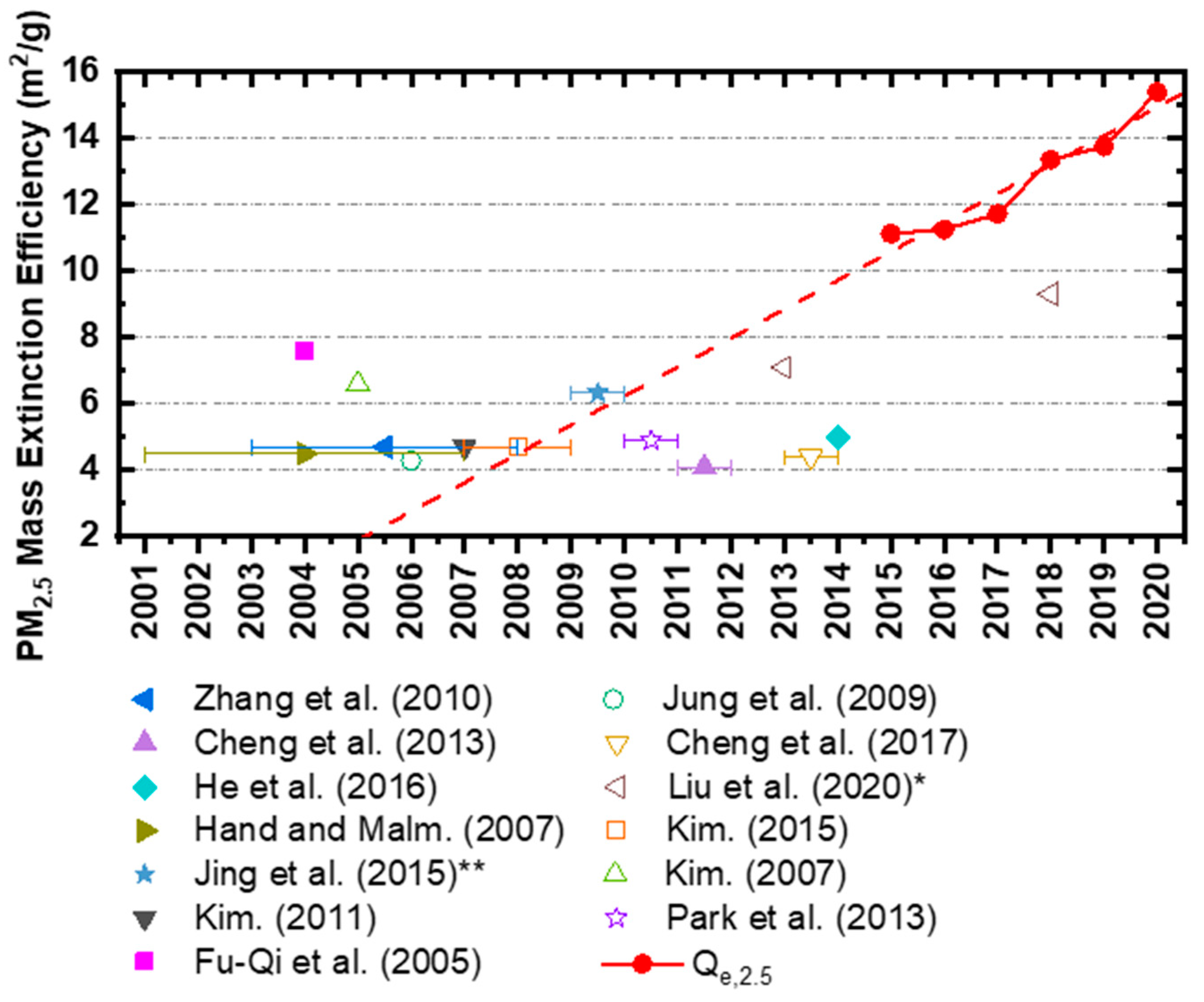
4.2. Q_e,2.5 Data Comparison

Figure 8 shows the Q_e,2.5 value reported in previous studies conducted in Northeast Asia compared with the Q_e,2.5 value obtained in this study [27,30,39,40,50,52,53,54,55,56,57,58,59]. As some studies showed only the mass scattering efficiency value, the Q_e,2.5 value was calculated again using the empirical SSA value of 0.8 as in Cheng et al. (2017) [39]. Other studies used a wavelength of 550 nm except for Liu et al. (2020) [27] and Jing et al. (2015) [54] that used wavelengths of 589 and 525 nm, respectively. Liu et al. (2020) [27] showed that the PM_2.5 decreased from 2013 to 2018, but the Q_e,2.5 value in 2018 increased compared to that in 2013 due to an increase in the proportion of aerosol nitrate and an increase in relative humidity. Similar to the observation of increase in Q_e,2.5 by Liu et al. (2020) [27] in eastern China, our results also indicate increasing trend of Q_e,2.5 in most of the regions in this study compared to the past data. The data from our study confirms the long-term increasing trend of Q_e,10 and Q_e,2.5. This trend of increasing Q_e,2.5 is similar to the result of shin et al. (2022) [60].

Many previous studies related to Q_e found that light extinction caused by particles is affected by particle properties such as size, composition, or meteorological factors such as relative humidity. Q_e varies depending on the diameter of the particle, and Q_e of PM_2.5 is approximately three times higher than that of PM₁₀ [36,37]. In addition, Q_e varies according to the mass ratio of components of PM_2.5, and Q_e increases as the mass fraction of carbonaceous substances and secondary inorganic species with high hygroscopicity (sulfate, nitrate, and ammonia) increase [39].

5. Conclusions

This study examined the long-term trends in Q_e, one of the optical characteristics of PM, using PM₁₀ and visibility data from 2001 to 2020 and PM_2.5 from 2015 to 2020 in Korea. Looking at annual Q_e, Q_e,10 increased from 0.06 to 0.22 (m²/g)/yr in all cities except Jeju. However, statistical test results for Chuncheon and Jeju showed a CL less than 95%. Q_e,2.5 increased in all cities from 0.28 to 2.47 (m²/g)/yr, but only Wonju, Busan, and Jeju had a CL higher than 95%. The monthly Q_e,2.5 increased from 0.04 to 0.23 (m²/g)/mth, and the statistical test result had a CL higher than 95% in all cities except Suwon. Finally, after dividing the PM₁₀ and PM_2.5 data into low, moderate, and high concentrations, Q_e changes were observed. When PM₁₀ was at a low concentration (19–21 μg/m³), Q_e,10 showed a tendency to decrease. Contrarily, Q_e,10 in most cities showed an increasing trend at moderate concentration (69–71 μg/m³) and high concentration (139–141 μg/m³). Q_e,2.5 increased in most cities except for Suwon and Pohang at low (9–11 μg/m³), moderate (29–31 μg/m³), and high concentration (69–71 μg/m³). However, in the case of, Q_e,2.5 of Seoul showed a decreasing trend for high concentrations but Q_e,2.5 remained high throughout the study period, which differed from other cities.

The increasing trend of Q_e shown in this study indicates that PM particle size and composition are changing in ways that are causing Q_e to increase. The increase in the Q_e value means that even if the amount of PM is reduced by various policies, citizens do not necessarily experience or report proportional improvement in visibility and may feel that such polices have not been effective. Therefore, to increase the effect of PM reduction and make effective PM–related policies, it is necessary to consider the particle size and composition of PM as well as its mass concentration. Additional research is needed to understand the change in particle size or composition so that the cause of the increase in Q_e can be identified.

References

1. Cao, J.-J.; Wang, Q.-Y.; Chow, J.C.; Watson, J.G.; Tie, X.-X.; Shen, Z.-X.; Wang, P.; An, Z.-S. Impacts of aerosol compositions on visibility impairment in Xi’an, China. Atmos. Environ. 2012, 59, 559–566. [Google Scholar] [CrossRef]
2. Charlson, R.J.; Schwartz, S.E.; Hales, J.M.; Cess, R.D.; Coakley, J.A., Jr.; Hansen, J.E.; Hofmann, D.J. Climate forcing by anthropogenic aerosols. Science 1992, 255, 423–430. [Google Scholar] [CrossRef] [PubMed]
3. Feng, S.; Gao, D.; Liao, F.; Zhou, F.; Wang, X. The health effects of ambient PM2.5 and potential mechanisms. Ecotoxicol. Environ. Saf. 2016, 128, 67–74. [Google Scholar] [CrossRef] [PubMed]
4. Pui, D.Y.H.; Chen, S.-C.; Zuo, Z. PM2.5 in China: Measurements, sources, visibility and health effects, and mitigation. Particuology 2014, 13, 1–26. [Google Scholar] [CrossRef]
5. Ramanathan, V.; Feng, Y. Air pollution, greenhouse gases and climate change: Global and regional perspectives. Atmos. Environ. 2009, 43, 37–50. [Google Scholar] [CrossRef]
6. Ramanathan, V.; Vogelmann, A.M. Greenhouse effect, atmospheric solar absorption and the Earth’s radiation budget: From the Arrhenius-Langley era to the 1990s. Ambio J. Hum. Environ. 1997, 26, 38–46. [Google Scholar]
7. Wang, J.L.; Zhang, Y.H.; Shao, M.; Liu, X.L.; Zeng, L.M.; Cheng, C.L.; Xu, X.F. Quantitative relationship between visibility and mass concentration of PM2.5 in Beijing. J. Environ. Sci. 2006, 18, 475–481. [Google Scholar]
8. Dockery, D.W.; Pope, C.A. Acute respiratory effects of particulate air pollution. Annu. Rev. Public Health 1994, 15, 107–132. [Google Scholar] [CrossRef]
9. Laden, F.; Schwartz, J.; Speizer, F.E.; Dockery, D.W. Reduction in fine particulate air pollution and mortality: Extended follow-up of the Harvard six Cities study. Am. J. Respir. Crit. Care Med. 2006, 173, 667–672. [Google Scholar] [CrossRef]
10. Polichetti, G.; Cocco, S.; Spinali, A.; Trimarco, V.; Nunziata, A. Effects of particulate matter (PM10, PM2.5 and PM1) on cardiovascular system. Toxicology 2009, 261, 1–8. [Google Scholar] [CrossRef]
11. Pope, C.A., 3rd; Dockery, D.W. Health effects of fine particulate air pollution: Lines that connect. J. Air Waste Manag. Assoc. 2006, 56, 709–742. [Google Scholar] [CrossRef] [PubMed]
12. Xing, Y.F.; Xu, Y.H.; Shi, M.H.; Lian, Y.X. The impact of PM2.5 on the human respiratory system. J. Thorac. Dis. 2016, 8, E69–E74. [Google Scholar] [PubMed]
13. IARC. IARC: Outdoor Air Pollution a Leading Environmental Cause of Cancer Deaths; World Health Organization: Geneva, Switzerland, 2013; pp. 1–4. [Google Scholar]
14. Huang, Y.; Shen, H.; Chen, H.; Wang, R.; Zhang, Y.; Su, S.; Chen, Y.; Lin, N.; Zhuo, S.; Zhong, Q.; et al. Quantification of global primary emissions of PM2.5, PM10, and TSP from combustion and industrial process sources. Environ. Sci. Technol. 2014, 48, 13834–13843. [Google Scholar] [CrossRef] [PubMed]
15. Lee, S.; Ho, C.-H.; Lee, Y.G.; Choi, H.-J.; Song, C.-K. Influence of transboundary air pollutants from China on the high- PM10 episode in Seoul, Korea for the period October 16–20, 2008. Atmos. Environ. 2013, 77, 430–439. [Google Scholar] [CrossRef]
16. Park, Y.M.; Park, K.S.; Kim, H.; Yu, S.M.; Noh, S.; Kim, M.S.; Kim, J.Y.; Ahn, J.Y.; Lee, M.D.; Seok, K.S.; et al. Characterizing isotopic compositions of TC-C, NO3-N, and NH4+-N in PM2.5 in South Korea: Impact of China’s winter heating. Environ. Pollut. 2018, 233, 735–744. [Google Scholar] [CrossRef]
17. Dehkhoda, N.; Noh, Y.; Joo, S. Long-Term Variation of Black Carbon Absorption Aerosol Optical Depth from AERONET Data over East Asia. Remote Sens. 2020, 12, 3551. [Google Scholar] [CrossRef]
18. Dehkhoda, N.; Sim, J.; Joo, S.; Shin, S.; Noh, Y. Retrieval of Black Carbon Absorption Aerosol Optical Depth from AERONET Observations over the World during 2000–2018. Remote Sens. 2022, 14, 1510. [Google Scholar] [CrossRef]
19. Ding, A.; Huang, X.; Nie, W.; Chi, X.; Xu, Z.; Zheng, L.; Xu, Z.; Xie, Y.; Qi, X.; Shen, Y.; et al. Significant reduction of PM2.5 in eastern China due to regional-scale emission control: Evidence from SORPES in 2011–2018. Atmos. Chem. Phys. 2019, 19, 11791–11801. [Google Scholar] [CrossRef] [Green Version]
20. Ito, A.; Wakamatsu, S.; Morikawa, T.; Kobayashi, S. 30 years of air quality trends in Japan. Atmosphere 2021, 12, 1072. [Google Scholar] [CrossRef]
21. Yamagami, M.; Ikemori, F.; Nakashima, H.; Hisatsune, K.; Ueda, K.; Wakamatsu, S.; Osada, K. Trends in PM2.5 Concentration in Nagoya, Japan, from 2003 to 2018 and impacts of PM2.5 countermeasures. Atmosphere 2021, 12, 590. [Google Scholar] [CrossRef]
22. Lang, J.; Zhang, Y.; Zhou, Y.; Cheng, S.; Chen, D.; Guo, X.; Chen, S.; Li, X.; Xing, X.; Wang, H. Trends of PM2.5 and chemical composition in Beijing, 2000–2015. Aerosol Air Qual. Res. 2017, 17, 412–425. [Google Scholar] [CrossRef]
23. Fontes, T.; Li, P.; Barros, N.; Zhao, P. Trends of PM2.5 Concentrations in China: A long term approach. J. Environ. Manag. 2017, 196, 719–732. [Google Scholar] [CrossRef] [PubMed]
24. Hara, K.; Homma, J.; Tamura, K.; Inoue, M.; Karita, K.; Yano, E. Decreasing trends of suspended particulate matter and PM2.5 Concentrations in Tokyo, 1990–2010. J. Air Waste Manag. Assoc. 2013, 63, 737–748. [Google Scholar] [CrossRef] [PubMed] [Green Version]
25. Yeo, M.J.; Kim, Y.P. Trends of the PM10 concentrations and high PM10 concentration cases in Korea. J. Korean Soc. Atmos. Environ. 2019, 35, 249–264. [Google Scholar] [CrossRef]
26. Xu, W.; Kuang, Y.; Bian, Y.; Liu, L.; Li, F.; Wang, Y.; Xue, B.; Luo, B.; Huang, S.; Yuan, B.; et al. Current challenges in visibility improvement in southern China. Environ. Sci. Technol. Lett. 2020, 7, 395–401. [Google Scholar] [CrossRef]
27. Liu, J.; Ren, C.; Huang, X.; Nie, W.; Wang, J.; Sun, P.; Chi, X.; Ding, A. Increased aerosol extinction efficiency hinders visibility improvement in eastern China. Geophys. Res. Lett. 2020, 47, e2020GL090167. [Google Scholar] [CrossRef]
28. Korea Environment Institute. Particulate Matter Perception Survey; KEI Focus, Republic of Korea: Sejong, Korea, 2019. [Google Scholar]
29. Koschmieder, H. Theorie der horizontalen Sichtweite. Beitrage zur Physik der freien Atmosphare. Meteorol. Z. 1924, 12, 3353. [Google Scholar]
30. Kim, K.W. Optical properties of size-resolved aerosol chemistry and visibility variation observed in the urban site of Seoul, Korea. Aerosol Air Qual. Res. 2015, 15, 271–283. [Google Scholar] [CrossRef] [Green Version]
31. Sloane, C.S.; Wolff, G.T. Prediction of ambient light scattering using a physical model responsive to relative humidity: Validation with measurements from Detroit. Atmos. Environ. 1985, 19, 669–680. [Google Scholar] [CrossRef]
32. Yuan, C.-S.; Lee, C.-G.; Liu, S.-H.; Chang, J.-c.; Yuan, C.; Yang, H.-Y. Correlation of atmospheric visibility with chemical composition of Kaohsiung aerosols. Atmos. Res. 2006, 82, 663–679. [Google Scholar] [CrossRef]
33. Khanna, I.; Khare, M.; Gargava, P.; Khan, A.A. Effect of PM2.5 chemical constituents on atmospheric visibility impairment. J. Air Waste Manag. Assoc. 2018, 68, 430–437. [Google Scholar] [CrossRef] [PubMed] [Green Version]
34. Yang, L.X.; Wang, D.C.; Cheng, S.H.; Wang, Z.; Zhou, Y.; Zhou, X.H.; Wang, W.X. Influence of meteorological conditions and particulate matter on visual range impairment in Jinan, China. Sci. Total Environ. 2007, 383, 164–173. [Google Scholar] [CrossRef] [PubMed]
35. Yu, X.; Ma, J.; An, J.; Yuan, L.; Zhu, B.; Liu, D.; Wang, J.; Yang, Y.; Cui, H. Impacts of meteorological condition and aerosol chemical compositions on visibility impairment in Nanjing, China. J. Clean. Prod. 2016, 131, 112–120. [Google Scholar] [CrossRef]
36. Jung, C.H.; Um, J.; Bae, S.Y.; Yoon, Y.J.; Lee, S.S.; Lee, J.Y.; Kim, Y.P. Analytic expression for the aerosol mass efficiencies for polydispersed accumulation mode. Aerosol Air Qual. Res. 2018, 18, 1503–1514. [Google Scholar] [CrossRef] [Green Version]
37. Kim, K.; Kim, Y. Opto-chemical characteristics of visibility impairment using semi-continuous aerosol monitoring in an urban area during summertime. J. Korean Soc. Atmos. Environ. 2003, 19, 647–661. [Google Scholar]
38. Qu, W.J.; Wang, J.; Zhang, X.Y.; Wang, D.; Sheng, L.F. Influence of relative humidity on aerosol composition: Impacts on light extinction and visibility impairment at two sites in coastal area of China. Atmos. Res. 2015, 153, 500–511. [Google Scholar] [CrossRef]
39. Cheng, Z.; Ma, X.; He, Y.; Jiang, J.; Wang, X.; Wang, Y.; Sheng, L.; Hu, J.; Yan, N. Mass extinction efficiency and extinction hygroscopicity of ambient PM2.5 in urban China. Environ. Res. 2017, 156, 239–246. [Google Scholar] [CrossRef]
40. He, Q.; Zhou, G.; Geng, F.; Gao, W.; Yu, W. Spatial distribution of aerosol hygroscopicity and its effect on PM2.5 Retrieval in East China. Atmos. Res. 2016, 170, 161–167. [Google Scholar] [CrossRef]
41. Lin, C.; Li, Y.; Yuan, Z.; Lau, A.K.H.; Li, C.; Fung, J.C.H. Using satellite remote sensing data to estimate the high-resolution distribution of ground-level PM2.5. Remote Sens. Environ. 2015, 156, 117–128. [Google Scholar] [CrossRef]
42. Tang, I.N. Chemical and size effects of hygroscopic aerosols on light scattering coefficients. J. Geophys. Res. Atmos. 1996, 101, 19245–19250. [Google Scholar] [CrossRef]
43. Zhao, P.; Zhang, X.; Xu, X.; Zhao, X. Long-term visibility trends and characteristics in the region of Beijing, Tianjin, and Hebei, China. Atmos. Res. 2011, 101, 711–718. [Google Scholar] [CrossRef]
44. Sun, X.; Zhao, T.; Liu, D.; Gong, S.; Xu, J.; Ma, X. Quantifying the influences of PM2.5 and relative humidity on change of atmospheric visibility over recent winters in an urban area of East China. Atmosphere 2020, 11, 461. [Google Scholar] [CrossRef]
45. Kendall, M. Rank Correlation Methods; Charles Griffin: London, UK, 1975. [Google Scholar]
46. Mann, H.B. Spatial-temporal variation and protection of wetland resources in Xinjiang. Econometrica 1945, 13, 245–259. [Google Scholar] [CrossRef]
47. Sen, P.K. Estimates of the regression coefficient based on Kendall’s tau. J. Am. Stat. Assoc. 1968, 63, 1379–1389. [Google Scholar] [CrossRef]
48. Cho, J.H.; Kim, H.S.; Chung, Y.S. Spatio-temporal changes of PM10 trends in South Korea caused by East Asian atmospheric variability. Air Qual. Atmos. Health 2021, 14, 1001–1016. [Google Scholar] [CrossRef]
49. Wan, Z.; Zhu, M.; Chen, S.; Sperling, D. Pollution: Three steps to a green shipping industry. Nature 2016, 530, 275–277. [Google Scholar] [CrossRef]
50. Cheng, Z.; Wang, S.; Jiang, J.; Fu, Q.; Chen, C.; Xu, B.; Yu, J.; Fu, X.; Hao, J. Long-term trend of haze pollution and impact of particulate matter in the Yangtze River Delta, China. Environ. Pollut. 2013, 182, 101–110. [Google Scholar] [CrossRef]
51. Husar, R.B.; Falke, S.R. The Relationship between Aerosol Light Scattering and Fine Mass; Report No. CX 824179-01; Center for Air Pollution Impact and Trend Analysis (CAPITA): St. Louis, MO, USA, 1996. [Google Scholar]
52. Zhang, Q.H.; Zhang, J.P.; Xue, H.W. The challenge of improving visibility in Beijing. Atmos. Chem. Phys. 2010, 10, 7821–7827. [Google Scholar] [CrossRef] [Green Version]
53. Hand, J.L.; Malm, W.C. Review of aerosol mass scattering efficiencies from ground-based measurements since 1990. J. Geophys. Res. Atmos. 2007, 112, D16203. [Google Scholar] [CrossRef]
54. Jing, J.; Wu, Y.; Tao, J.; Che, H.; Xia, X.; Zhang, X.; Yan, P.; Zhao, D.; Zhang, L. Observation and analysis of near-surface atmospheric aerosol optical properties in urban Beijing. Particuology 2015, 18, 144–154. [Google Scholar] [CrossRef]
55. Kim, K.W. Time-resolved chemistry measurement to determine the aerosol optical properties using PIXE analysis. J. Korean Phys. Soc. 2011, 59, 189–195. [Google Scholar] [CrossRef]
56. Si, F.-Q.; Liu, J.; Xie, P.-H.; Zhang, Y.-J.; Liu, W.-Q.; Kuze, H.; Cheng, L.; Takeuchi, N.; Lagrosas, N. Determination of aerosol extinction coefficient and mass extinction efficiency by DOAS with a flashlight source. Chin. Phys. 2005, 14, 2360. [Google Scholar]
57. Jung, J.; Lee, H.; Kim, Y.J.; Liu, X.; Zhang, Y.; Gu, J.; Fan, S. Aerosol chemistry and the effect of aerosol water content on visibility impairment and radiative forcing in Guangzhou during the 2006 Pearl River Delta campaign. J. Environ. Manag. 2009, 90, 3231–3244. [Google Scholar] [CrossRef] [PubMed]
58. Kim, K.W. Physico-chemical characteristics of visibility impairment by airborne pollen in an urban area. Atmos. Environ. 2007, 41, 3565–3576. [Google Scholar] [CrossRef]
59. Park, S.S.; Kim, K.W.; Schauer, J.J. Influence of hydrophilic and hydrophobic water-soluble organic carbon fractions on light extinction at an urban site. J. Korean Phys. Soc. 2013, 63, 2047–2053. [Google Scholar] [CrossRef]
60. Shin, J.; Kim, D.; Noh, Y. Estimation of Aerosol Extinction Coefficient Using Camera Images and Application in Mass Extinction Efficiency Retrieval. Remote Sens. 2022, 14, 1224. [Google Scholar] [CrossRef]
Figure 1. Location of cities studied.
Remotesensing 14 01592 g001
Figure 2. Eight cities’ annual average and trend in visibility and PM10 2001–2020.
Remotesensing 14 01592 g002
Figure 3. Eight cities’ annual average and trend in visibility and PM2.5 in 2015–2020.
Remotesensing 14 01592 g003
Figure 4. Qe,10 annual average and trend 2001–2020.
Remotesensing 14 01592 g004
Figure 5. Qe,2.5 annual average and trend 2015–2020.
Remotesensing 14 01592 g005
Figure 6. Qe,2.5 monthly average and trend from 2015 to 2020.
Remotesensing 14 01592 g006
Figure 7. Change in Qe for each concentration category of PM10 and PM2.5 in each city. PM10: (a) 19–21 μg/m3 (low), (b) 69–71 μg/m3 (moderate), (c) 139–141 μg/m3 (high); PM2.5: (d) 9–11 μg/m3 (low), (e) 29–31 μg/m3 (moderate), (f) 69–71 μg/m3 (high).
Remotesensing 14 01592 g007
Figure 8. Comparison of Qe,2.5 values from this and previous studies at wavelength 550 nm. * Used wavelength 589 nm. ** Used wavelength 525 nm.
Remotesensing 14 01592 g008