Abstract
The accurate simulation of microwave observations of clouds and precipitation are computationally challenging. A common simplification is the assumption of totally random orientation (TRO); however, studies have revealed that TRO occurs relatively infrequently in reality. A more appropriate assumption is that of azimuthally random orientation (ARO), but so far it has been a computationally expensive task. Recently a fast approximate approach was introduced that incorporates hydrometeor orientation into the assimilation of data from microwave conically scanning instruments. The approach scales the extinction in vertical (V) and horizontal (H) polarised channels to approximate ARO. In this study, the application of the approach was extended to a more basic radiative transfer perspective using the Atmospheric Radiative Transfer Simulator and the high-frequency channels of the Global Precipitation Measurement Microwave Imager (GMI). The comparison of forward simulations and GMI observations showed that with a random selection of scaling factors from a uniform distribution between 1 and 1.4–1.5, it is possible to mimic the full distribution of observed polarisation differences at 166 GHz over land and water. The applicability of this model at 660 GHz was also successfully demonstrated by means of existing airborne data. As a complement, a statistical model for polarised snow emissivity between 160 and 190 GHz was also developed. Combining the two models made it possible to reproduce the polarisation signals that were observed over all surface types, including snow and sea ice. Further, we also investigated the impact of orientation on the ice water path (IWP) retrievals. It has been shown that ignoring hydrometeor orientation has a significant negative impact (∼20% in the tropics) on retrieval accuracy. The retrieval with GMI observations produced highly realistic IWP distributions. A significant highlight was the retrieval over snow covered regions, which have been neglected in previous retrieval studies. These results provide increased confidence in the performance of passive microwave observation simulations and mark an essential step towards developing the retrievals of ice hydrometeor properties based on data from GMI, the Ice Cloud Imager (ICI) and other conically scanning instruments.
1. Introduction
Microwave radiometry is recognised as an efficient approach for observing surface precipitation rates and hydrometeor column contents due to its ability to probe the interior of cloudy air masses [1,2]. Liquid water content and rain rates are typically measured at frequencies up to 90 GHz, while in general, sensitivity to frozen hydrometeors requires higher frequencies. Space-based microwave sensors (excluding limb sounding) today cover 6 to 190 GHz and various parts of this frequency range have been used to improve our understanding of cloud and precipitation processes [3,4,5,6,7]. Numerical weather prediction (NWP) has also benefited from all-sky microwave radiances through recent developments in data assimilation techniques [8].
Frozen hydrometeors interact with microwave radiation both through scattering and absorption. Scattering by oriented hydrometeors is characterised by strong dichroism effects [9,10,11,12,13,14], which result in brightness temperature (TB) differences between the radiances measured at vertical (V) and horizontal (H) polarisations. This deviation (TB−TB) is known as the polarisation difference (PD). In reality, PDs depend on microphysical properties, e.g., the size, shape and orientation of the hydrometeors. Thus, a complex mixture of hydrometeor in the atmosphere can generate a plethora of polarisation signals. Additionally, PDs also arises due to the polarisation-dependent emission and scattering of liquid hydrometeors and the surface (typically water).
Spencer et al. [15] were the first to report observed PDs, which were found at 37 GHz during heavy thunderstorm events over land. Later, Prigent et al. [16] analysed observations at 37 and 85 GHz and identified polarisation signatures that corresponded to convective systems and stratiform anvils. At higher microwave frequencies (157 GHz), Defer et al. [17] found PD values of up to 10 K in the tropics. Ground-based sensors operating at 150 GHz have also observed PDs of up to 10 K during snowfall events [18]. Gong and Wu [19] and Galligani et al. [20] made a similar analysis for larger geographical areas using the Global Precipitation Measurement (GPM) Microwave Imager (GMI). They found that the variation of PD as a function of TB exhibits a relatively constant arch-shape pattern that is independent from latitude. The arch-like shape is governed by two processes: the presence of various hydrometeors in turbulent flow and the saturation of polarisation signals under multiple scattering. The highest PDs arise from hydrometeors in low turbulence conditions, such as anvils and stratiform regions [19]. However, multiple scattering processes from multiple hydrometeors eventually lead to a polarisation signal saturation. The lowest PDs are associated with convective zones, where turbulent motions cause hydrometeors to be randomly oriented in addition to the increased multiple scattering processes.
The well-established impact of the oriented hydrometeors has encouraged several authors to emphasise the need for the incorporation of hydrometeor orientation into retrievals, based on microwave data [17,19,21,22,23]. This has not yet occurred. In simulated retrievals, Jiménez et al. [24] made a smaller, inconclusive test to incorporate hydrometeor orientation, while others have consistently assumed a totally random orientation (TRO) of the ice hydrometeors. Spherical hydrometeors are also covered under TRO. When TRO is not applied, it is generally believed that ice hydrometeors exhibit azimuthally random orientation (ARO) [13]. The ARO concept means that there is no preferred orientation in azimuth, but that the hydrometeors have some distribution in the angle between the horizon and the reference plane of the hydrometeors. The main deviation to ARO should be the alignment with electrical fields in thunderstorms [25].
One reason that oriented hydrometeors have been ignored in microwave retrievals is because the consideration of such hydrometeors requires a polarised (vector) radiative transfer, which is more computationally intensive than the standard unpolarised (scalar) calculations. There are vector software packages available [26,27,28,29], but only a few [13,30] have studied the dichroism effects that are exhibited by oriented hydrometeors. The lack of realistic scattering property data in the ARO category has been an even more significant limiting factor [31]. Some such data were developed and explored by Adams and Bettenhausen [32]. The first publicly available data were provided by Brath et al. [13], but only for two hydrometeor shapes (habits). This is in contrast with the main part of the accompanying scattering database that covers TRO with 36 shapes [33]. This striking difference is explained by the fact that ARO requires much more resources, both in terms of the production and storage of the data.
Despite existing tools and data allowing for rigorous simulations that reproduce the PDs seen in GMI data [13], the situation remains unsatisfactory. While it has been possible to exploit the polarisation signals that are observed at low frequencies in studies of precipitation and mixed-phase clouds [34,35,36], a scalar radiative transfer is still preferred (or is a demand) in many applications involving ice hydrometeors. Falling liquid droplets can also be characterised by ARO. This is attributed to the flattening that is induced by air drag. However, liquid particles (i.e., rain drops and cloud droplets) are well approximated by spheroids and hence, they are relatively easy to handle [37]. On the contrary, the radiative properties of ice hydrometeors vary strongly with shape [38] and the data provided by Brath et al. [13] are not sufficient to represent all hydrometeor types or perform a search for a “best fit” shape, as performed by Geer [39].
As a consequence of these reasons, approaches for the approximation of the ARO case have been investigated. Galligani et al. [20] attempted to parametrise the polarisation signals that were observed from GMI at 89 and 166 GHz with good results. However, their method is limited to only these two frequencies as it requires actual dual-polarisation observations for the frequency to be simulated. For instance, the GMI 183 GHz channels are V polarised and a correction for these channels cannot be presented due to the lack of parallel H polarised channels. Further, an extension of their approach to sub-millimetre (sub-mm) wavelengths is not viable today due to the lack of observational data. A more physically-based method to approximate the polarisation signatures was introduced by Barlakas et al. [14]. Their method mimics the effect of ARO hydrometeors through scaling the TRO optical properties for H and V polarised channels by a factor known as the polarisation ratio (). They demonstrated an improved representation of all-sky microwave radiances in an NWP system (Integrated Forecast System, IFS) by introducing a constant scaling factor into the radiative transfer tool that was applied (radiative transfer for TOVS microwave and sub-millimetre scattering code, RTTOV-SCATT). Their method applies to other radiative transfer models and applications, but the selection of the polarisation ratio must be readdressed (as discussed below).
The need to improve hydrometeor representation increases with the launch of new sensors, such as the Ice Cloud Imager [40] (ICI). ICI is the first operational radiometer measuring in the sub-mm region at frequencies up to 664 GHz. The radiances are directly ingested into NWP models, but stand-alone retrievals to derive a range of geophysical quantities are also seen. While there have been preparatory steps towards the development of ICI retrieval databases [40,41], all of these studies have assumed TRO. For realistic simulations, ARO must be incorporated at all frequencies, irrespective of the fact of whether they are dual-polarised or not. While dual-polarisation channels may be the best for visualising and analysing the polarisation signals, oriented hydrometeors have an impact on all channels.
In this study, we aimed to provide a pragmatic solution to a limitation in microwave radiative transfer. The approach is of general interest for conically scanning instruments and could be applied in, for example, a satellite simulator. Another application is the production of high-quality retrieval databases and to allow, for example, future ICI observations to be used to their full potential. Our specific objective was in this direction: to include ARO in a retrieval database and validate its ability to statistically reproduce observed PD signatures.
We utilised the high-frequency channels of GMI to demonstrate and extend the scheme developed by Barlakas et al. [14] in order to incorporate ARO into single-footprint data. In their study, they found that is the best performing scaling factor at 166 GHz. However, this value cannot be used directly in other applications. Firstly, the GMI observations were “superobbed” to a resolution of 80 km × 80 km, following the way in which data from conically scanning instruments are assimilated at the European Centre for Medium-Range Weather Forecasts (ECMWF). Lowering the resolution smeared out the maximum and minimum PDs compared to what is observed at native resolution (i.e., a pixel size of ∼6 km at nadir). Furthermore, using a constant value of does not reproduce the full PD distribution, which should be the aim, at least when generating retrieval databases. Additionally, the limitations of the radiative transfer tool (RTTOV-SCATT) could also have some influence.
With the revision of the scaling scheme, we generated a database consisting of a large number of atmospheric states. The target was to fully represent the PD signatures that are generated by ice hydrometeors in a statistical sense and to quantify the benefits of incorporating ARO into the retrievals of ice water path (IWP). Errors caused by assuming TRO were assessed by simulations, while GMI measurement data were used to show that the retrieval database that was created does indeed work in practice. Additionally, the performance of the scheme at 660 GHz was investigated and compared to available airborne data.
2. Satellite and Model Data
2.1. Global Precipitation Measurement Microwave Imager
The Global Precipitation Measurement (GPM) Microwave Imager (GMI) instrument is a conically scanning microwave radiometer that measures 13 frequencies ranging from 10 GHz to 183 GHz. The instrument has an Earth incidence angle of 52.8° for frequencies up to 89 GHz and 49.1° for the 166 GHz and 183 GHz channels. In this study, we only used the four high-frequency channels between 166 GHz and 183 GHz (Table 1). The high-frequency channels have a swath width of 885 km and the orbit covers a latitude range from 65°S to 65°N. These channels are the most sensitive to precipitating ice and water vapour and have instantaneous footprints of 4.4 km × 7.2 km. The GMI dataset in this study was used for the Level 1 raw radiance measurements [42] (L1B).

Table 1.
The specifications of the Global Precipitation Measurement (GPM) Microwave Imager (GMI) channels that are relevant to this study. V and H denote vertical and horizontal polarisation.
Additionally, ancillary data, such as surface classification, 2 m temperature and water vapour path, were also used in correspondence with L1B radiances. These data are available as a part of the GPM Goddard profiling algorithm [43] (GPROF).
2.2. Ice Cloud Imager
The Ice Cloud Imager (ICI) is a new microwave conically scanning radiometer that has 13 channels that measure 11 frequencies from 183 GHz to 664 GHz [40]. It is a part of the next generation of the European Organisation for the Exploitation of Meteorological Satellites Polar System, Second Generation (EUMETSAT EPS-SG), which is scheduled to be launched in 2025. The instrument observes Earth with an Earth incidence angle of 53 and a swath width of 1700 km. The instantaneous footprints are about 16 km. The main objective of ICI is to improve the retrieval of ice hydrometeors and their representation in regional and global NWP models using high-frequency channels and thus, extend the scope of data assimilation.
2.3. CloudSat
The CloudSat is a sun-synchronous satellite that was part of the A-train constellation and has provided information on the vertical structure of clouds and aerosols since 2006. It carries a 94 GHz Cloud Profiling Radar (CPR) to measure the backscattering caused by clouds. It has a vertical resolution of 485 m and a 1.8 km along-track and 1.2 km cross-track resolution. The CloudSat data used in this study are radar reflectivities from the 2B GEOPROF R05 product [44].
In 2011, CPR suffered from a battery anomaly and has only operated in daylight mode since then. To avoid any bias due to only operating in the daytime, we utilised CloudSat profiles from 2009. The data were constrained to 65°S and 65°N to match the GMI latitudinal coverage.
2.4. ERA5
ERA5 holds the global reanalysis data that are provided by the ECMWF [45]. The reanalysis combines the model data with observations to provide hourly estimates of various atmospheric, ocean and land-surface variables. In this study, we uses multiple ERA5 atmospheric and surface parameters to generate the atmospheric scenes that were used as inputs for the radiative transfer simulations (Section 3.1.1). The parameters used were temperature, cloud liquid water content, specific humidity, 2 m temperature, 10 m u wind, 10 m v wind, land-sea mask, snow depth, sea ice fraction and surface elevation.
3. Tools and Methodology
3.1. Radiative Transfer Simulations
3.1.1. Atmospheric Scenarios
A database of two-dimensional (2D) scenes was created based on CloudSat radar reflectivities and ERA5 atmospheric and surface parameters. The radar reflectivities were inverted to obtain the vertical profiles of ice hydrometeors and rain by assuming a particle model (Section 3.1.2), while ERA5 provided the background data. Grids in pressure and latitude were defined. Each scene’s latitudinal grid was individually set to match the CloudSat data, while a custom vertical grid from −700 m to 20,000 m was defined. The vertical grid spacing was 125 m up to 8000 m and 250 m to beyond 8000 m. The ERA5 data closest to the CloudSat orbit (ascending or descending) were selected and interpolated into the CloudSat latitudinal grid. This approach to generating synthetic atmospheric scenes was essentially identical to that used by Ekelund et al. [41].
ERA5 was also used to define surface types. Land and water were classified using the ERA5 land-sea mask. The locations with a snow depth of more than 2 mm were classified as snow covered. The limit of 2 mm followed the wavelength of the GMI data that were used. We assumed a single snow surface type and the emissivities were set using a random snow emissivity model (Section 4.2). ERA5 describes the presence of sea ice using an areal coverage factor that has a resolution of about 25 km. These factors were mapped onto the database scenes for each 10 km (along the CloudSat orbit track) by randomly selecting sea ice and open water according to the sea ice fraction. For the rest, sea ice was treated as a part of the snow surface type, as there is a high probability that sea ice has some snow cover. Some additional constraints were also included in the database. All values of liquid water content below kg m or at a temperature lower than 248 K were set to zero.
3.1.2. ARTS Setup
All forward simulations were performed with the Atmospheric Radiative Transfer Simulator [46] (ARTS). The radiative transfer was performed in 2D view using an independent beam approximation, as described in Eriksson et al. [40], Barlakas and Eriksson [47]. The radar reflectivities were converted into hydrometeor bulk properties, ice water content (IWC) and rain water content (RWC), using a dbZ-based model system [41]. The microphysical assumptions are described in Section 3.1.3. CloudSat is not sensitive to cloud liquid water and provides no clear information on water phases. Thus, the temperature field was used to differentiate between liquid and ice hydrometeors. All hydrometeors below 273 K were classified as ice and all hydrometeors above 273 K were classified as rain. Supercooled liquid water was included in the simulations as liquid water content that was taken from ERA5. The radar measurements were inverted using an onion peeling concept. The method divided the atmosphere into layers and for each layer, measurements were inverted using an IWC-dbZ table. At each layer, the attenuation effects from hydrometeors and absorbing species were also considered and the radar reflectivities recorded at lower altitudes were corrected accordingly. For each layer, the hydrometeor attenuation was scaled by a factor of 0.4, following Figure 16 of [48], and the maximum value of correction that was allowed was 2. This upper limit helped to avoid any spurious cases of hydrometeor attenuation.
A zone of 1.2 km over land and 0.6 km over water was defined to avoid spurious water content due to surface clutter. All retrievals in this zone were rejected and instead, the value just above the clutter zone was used as a fill value. Despite the clutter filtering, a few cases of unfiltered clutter could exist and cause spuriously high IWC. The upper limit for retrieved IWC was set at 10 g m to avoid such retrievals. All retrievals above this threshold were set to zero. Additionally, all retrievals greater than 3 g m but less than 10 g m were clipped to 3 g m.
The land and water/ocean emissivities were taken from the Tool to Estimate Land-Surface Emissivities at Microwave frequencies [49] (TELSEM) and the Tool to Estimate Sea-Surface Emissivity from Microwaves to sub-millimetre waves [50] (TESSEM), respectively. As mentioned previously, emissivities for snow covered surfaces were calculated using an empirical snow emissivity model (Section 4.2).
3.1.3. Hydrometeor Properties
Three types of hydrometeors were considered for the radiative transfer calculation: cloud ice, rain and liquid clouds. The inversion of CloudSat reflectivities to IWC largely depends on the assumed microphysical properties; thus, we analysed the performance of two hydrometeor habits: large plate aggregate and Evans snow aggregate [6]. The large plate aggregate was used in a version where aggregates are complemented with the plate habit to cover smaller sizes. The size ranges for these habits are given in Table 2. In this study, most of the results were based on the large plate aggregate, but few results from the Evans snow aggregate are included in Appendix A. The single-scattering data were taken from the ARTS single-scattering database provided by Eriksson et al. [33] and the particle size distribution (PSD) developed by Field et al. [51] was also used. This PSD has two different distributions for the tropics and mid-latitudes, but we used the tropics setting for all latitudes following Geer et al. [38]. Henceforth, it is denoted as F07T. Rain was assumed as a liquid sphere and the PSD was from Marshall and Palmer [52].
Table 2.
The specifications of the two databases that were considered. Here, “aARO” denotes the approximated ARO hydrometeors. The two habits used in the study were aggregates and the size range covered was described by the volume equivalent diameter (D).
The absorption model included effects from five different species: nitrogen and oxygen [53], liquid water content [54], water vapour and ozone. For water vapour, we followed the absorption model in RTTOV [55], but with a few modifications as described by Turner et al. [56]. The liquid clouds were assumed to be totally absorbing and their scattering effects were neglected.
In this study, both ARO and TRO hydrometeors were simulated. The alternative way to approximate the hydrometeor orientation described by Barlakas et al. [14] was followed, but with some modifications (Section 4.1). Since this scheme approximated ARO behaviour without computing the fully polarised radiative transfer, hereafter in this study, the oriented hydrometeors are referred to as “approximated ARO” or “aARO”.
3.2. Generation of Databases
All simulations were performed in all-sky mode using the ARTS set-up described above. Only high-frequency GMI channels were simulated, i.e., 166V, 166H, 183 ± 3V and 183 ± 7V GHz. All simulations were based on CloudSat data from January 2009. The GMI antenna pattern was assumed to be a Gaussian footprint with full width at the half maximum of 6 km. Multiple pencil beam simulations were averaged over this pattern to yield the antenna brightness temperatures. During the averaging over GMI footprint, new mixed surface classes were also defined: coastlines, sea ice–water boundary, snow–land boundary, sea ice–land boundary and snow–water boundary.
Two type of databases were considered. The databases were identical in all aspects except orientation and habit. A summary of these databases is presented in Table 2. Additionally, to expand our study to sub-mm wavelengths, we included simulations at 660 GHz. An identical ARTS set-up (Section 3.1.2) was used for these simulations, but the surface was assumed to be a black body. Only one particle habit was tested as well, i.e., large plate aggregate. These simulations were performed for March 2009. All simulations were noise-free; so, to incorporate the measurement uncertainties, Gaussian noise was added according to the channel NET (Table 1).
Uncertainties in the inversions are dominated by the simplified microphysical assumptions and surface effects. Quantifying the database uncertainty was outside the scope of the present study. However, wherever possible, we tried to include the uncertainty due to the random sampling of the data. The uncertainty was calculated by bootstrapping, i.e., sampling with replacement.
3.3. Polarisation Ratio
Preferentially oriented hydrometeors exhibit strong dichroism effects (non-zero linear extinction cross-sections [12]), meaning that optical properties are viewing dependent. This results in significant differences in TBs being measured at V and H polarisations by microwave imagers. On the other hand, randomly oriented hydrometeors have no dichroism effects, i.e., the optical properties at V and H polarisations are identical. Hence, the polarisation signals are very small and only arise due to scattering effects e.g., [57].
At about 50–55°, which is the typical observation angle of conically scanning radiometers, orientation has a limited impact on most hydrometeor scattering properties. To demonstrate, Figure 1 shows the differences between the bulk optical properties of ARO and TRO as a function of the ice water path at 55°. It can be seen that the asymmetry parameter (Figure 1b) and the single-scattering albedo (Figure 1c) were marginally affected by hydrometeor orientation over the entire range of ice water content. Further, the ARO properties at both V and H were close to the TRO counterparts. This behaviour is broadly independent from the frequency. On the other hand, Figure 1a highlights the significant differences between the bulk extinction of V and H polarisation. These differences lead to the strong polarisation patterns that are measured by microwave imagers.
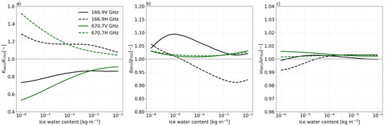
Figure 1.
For the large plate aggregate and the particle size distribution of Field et al. [51] (tropical configuration), the bulk optical properties of azimuth random orientation (ARO) at both V and H polarisation were normalised by the corresponding properties in case of total random orientation (TRO) as a function of the ice water content. The results are presented at an Earth incident angle of 55° at 166.9 and 670.7 GHz, based on (a) the extinction (K), (b) the asymmetry parameter (g) and (c) the single-scattering albedo (). For ARO, the single-scattering properties for a tilt angle of 0° were employed [13].
Accordingly, Barlakas et al. [14] introduced an approximate scheme to mimic the effect of hydrometeor orientation in the case of conical scanners. The scheme was based on a correction factor () that increases and decreases the layer bulk optical thickness () in the case of TRO, leading to the bulk () at H and V polarised channels, respectively. This is quantified by the so-called polarisation ratio that is given by:
In other words, the factor () weakens the bulk extinction at V polarisation and strengthens the bulk extinction at H polarisation, thereby approximating the bulk extinction of ARO hydrometeors (Figure 1a). The polarisation effects of preferentially oriented hydrometeors (due to aerodynamic and gravitational forces (e.g., [13,14] and references therein) are subject to their non-spherical shape. The ratio can be indirectly interpreted as the effective axial ratio of an oriented hydrometeor. Note here that the magnitude of strongly depends on the degree of orientation of the selected hydrometeor (shape) and Figure 1a depicts the maximum differences in the case of the large plate aggregate; for details, refer to Barlakas et al. [14]. For TRO, is equal to one () and for aARO, .
3.4. Retrieval Algorithm
The foremost objective of this study was to include hydrometeor orientation in radiative transfer simulations in a fast way. However, we also simultaneously attempted to retrieve IWPs from passive microwave observations. The idea was to combine the database of GMI simulations with a machine learning (ML) algorithm to retrieve IWP and quantify the impact of orientation on retrieval accuracy. Figure 2 provides a flowchart of the overall scheme that was followed.
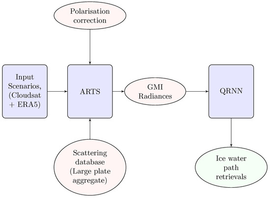
Figure 2.
The flowchart showing the retrieval system.
We based our retrievals on a neural network-based method called Quantile Regression Neural Network [58](QRNN). QRNN is available as the open-source software quantnn [59] and is implemented with PyTorch backend [60]. The QRNN architecture selected for this study is described in Appendix B. QRNN is trained using the information in the database to predict the posterior distribution of the quantity sought. A vector of quantiles describes the posterior distribution. This is different from the conventional ML retrieval methods that provide single-point estimates. The quantiles can also be used to quantify the prediction uncertainty for each case. While the posterior distribution has it own advantages, usually either the median quantile or the expectation value () is chosen as the point estimate for evaluating retrieval accuracy. In this study, the point comparisons were made with .
4. Results
This section first demonstrates the selection of the optimal polarisation ratio () through multiple experiments. The chosen was used to generate the retrieval databases and the database quality was analysed through comparisons to GMI observations. Later, the comparison of the IWP retrievals from both TRO- and aARO-based databases are described. It should be noted that some of the results presented are not one-to-one validations, but are instead statistical comparisons. Due to the non-availability of data from a common period, the data could belong to different years (but the same month). We emphasise that data from different years do not affect the statistical comparisons.
4.1. Polarisation Ratio
4.1.1. Overview
Barlakas et al. [14] found that the best estimate of the polarisation ratio ( at 166 GHz) by comparing multiple statistics between simulations and observations. They also compared the arch-shape relationship between PD and TB at V polarisation [19] (PD-TB) for simulations and observations. However, as mentioned earlier, their selection of could not be used directly in our study. In Barlakas et al. [14], the “superobbing” of the observations affected the full natural distribution of the PD-TB relationship. The averaging reduced the maximum PDs to ∼20 K, but for the same month (July), Gong and Wu [19] showed that PDs of up to ∼30 K exist over water. Similarly, the low PDs (< 5 K) were also affected. For the simulations, the majority of the low PDs were confined for TBs that were greater than 180 K. The simulated PDs that were associated with TBs of less than 180 K were also greater than 5 K. However, the observations show that low PDs exist over the entire TB range. The missing low PDs could also be the shortcoming of RTTOV-SCATT in correctly simulating the optical properties of hydrometeors that are associated with deep convection [14,39]. Furthermore, in NWP, the selection of is driven by observations at a given instance; the polarisation model should be correct for that time and position. However, in this study, we wanted to generate a retrieval database that demonstrates a larger variability. A constant value of cannot reproduce the full variability of observations. In this section, we readdress the selection of . Intuitively, the value of should still be close to that suggested by Barlakas et al. [14], but it requires a comparison of the distributions of forward-modelled radiances and observations.
Multiple experiments with different values of were conducted. All of these experiments had an identical set-up of microphysical assumptions for consistency. In the first five experiments, forward-modelled radiances were generated with . Two more experiments were also performed with values of that belonged to a uniform distribution and a truncated normal distribution. In these two experiments, the upper and lower limits of were motivated by the results from the first five experiments and details of this are described in the next section. Polarisation signals can also originate from the surface, but they were filtered out for this comparison. The “3” method described by Gong and Wu [19] was used to filter out the clear-sky cases. This method uses the TBs at 183 ± 3 GHz to define a threshold (T) and all cases with TBs < T are classified as cloudy. Here, was the standard deviation of the probability density function of the TBs. This stringent filtering could remove most of the cases that were affected by the surface, but at the cost of filtering thin cirrus cloud cases. For all of the analyses, we added instrument noise to the simulated radiances (Section 3.2).
4.1.2. Selecting the Optimal Polarisation Ratio
Figure 3 shows the PD-TB distribution over water and land. Here, the simulations did not have a one-to-one correspondence with the observations, but that was unnecessary. We were only interested in a statistical fit between the two distributions. The five experiments used simulations from the same month (January) but not identical synthetic scenes. Some statistical fluctuations due to inconsistencies between the datasets could be expected, but they should not significantly alter the overall behaviour. As Figure 3 only provides a qualitative view, we measured the divergence between the 2D histogram of the PD-TB distribution to quantify the measure of similarity between the observed and simulated PD-TB distributions. We employed the same method as that used by Barlakas et al. [14] to calculate the divergence. When and denote the populations for the observations and simulations in each bin and N is the total number of bins, then the divergence between the two is defined as:
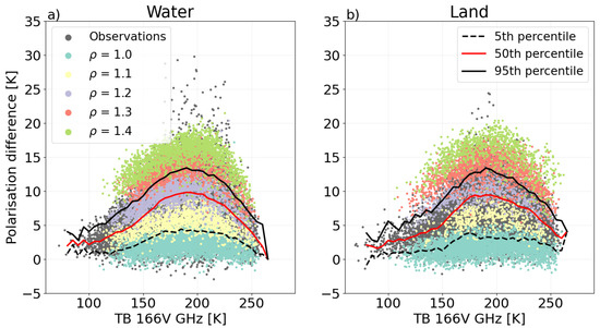
Figure 3.
The polarisation differences (166V − 166H) as a function of brightness temperatures at 166V GHz (PD-TB relationship) over (a) water and (b) land. The GMI observations are shown in dark grey, while the other colours represent the simulations for different values of . The three overlaid lines represent the 5th, 50th and 95th percentiles of the observed polarisation differences for each TB interval. The simulations were based on large plate aggregate. The data affected by the surface were filtered out (see text). The simulations were from January 2009 and the observations were from January 2017.
While estimating the 2D histograms, empty bins were replaced by a small number (10) to avoid infinite penalty. The divergence was calculated after removing the data that were affected by the surface and the results are provided in Table 3.
Table 3.
The 2D divergence describing the differences between the observations and simulations over water, land and all surface types. The results from the five experiments with different values of , uniform distribution ( U(1.0, 1.4)) and truncated normal distribution () are shown. The lowest divergences are highlighted in bold.
When , the simulations completely failed at reproducing the true PD-TB distribution. In this experiment, most simulations were associated with a small positive PD (0–3 K), but some cases with negative PDs were also present. The negative PDs were mostly due to differences in TB that arose from instrument noise. Further, the missing part of the arch distribution for TBs < 125 K was due to the limitation of the current set of microphysical assumptions. One particle habit and PSD combination is insufficient to accurately simulate the convective systems. The maximum PD that can be simulated with the TRO assumption is around 5 K, which is insufficient to recreate the observed PDs. As increases, the impact of orientation comes into the picture and higher PDs can be simulated. With , the maximum PD is around 12 K, which also reflects the median of PD-TB distribution [20]. Over water and with , most of the highest observed PDs (between 15 and 20 K) can be simulated, but PDs >20 K signals are missed. While > 1.4 can be included to reproduce the few cases with extremely high PDs (>20 K), it also increases the PDs over the slopes on either side of the arch peak. Some over-representation is already reflected for 1.3 and 1.4 in the regions with TB > 225 K and TB < 150 K. While it is acceptable to have some extra variability within the physical limits, selecting a constant seemed unfeasible with the current set of microphysical assumptions. This was also evident from the increase in divergence with increasing (Table 3). Over water, the 2D divergence increased from 1.62 for to 2.04 for . Similarly, over land, where the frequency of maximum observed PDs is smaller than over water, the values of > 1.4 could be ruled out.
Nevertheless, using a constant failed at reproducing realistic PD-TB distributions over both water and land and could only replicate a part of it. This suggests that a variation in is necessary to replicate the variety in polarisation signals. Based on the above results, we tested two different distributions for : a uniform distribution (U) between 1.0 and 1.4 and a truncated normal distribution () between 1.0 and 1.4, with a standard deviation of 0.12. Since replicated the PDs along the median, both distributions were centred around 1.2. The two distributions were expected to produce similar results, but the former simulated a slightly higher number of TRO cases and cases with high PDs.
The performance of U(1, 1.2) and was also evaluated through 2D divergence (Table 3). Over both water and land, selecting from a distribution produced a better match between the simulations and observations, as indicated by the lower divergence estimates. Among the two distributions, the uniform distribution emerged as having a better performance, but only by a small margin. This could be due to slightly better TB depressions and higher PDs. However, a truncated normal distribution with a larger variance is expected to produce comparable results. Ice scattering signatures over coastlines, snow, sea ice and other mixed surface types were neglected in deriving the optimal value of . However, we also evaluated the divergence when no surface type filtering was applied and a similar performance was achieved. For all subsequent results involving the large plate aggregate, U(1, 1.4) was used. Additionally, we also explored the effective range of for the Evans snow aggregate. These results are described in Appendix A.
Further, we also implemented a similar correction scheme for radar backscattering. A slightly smaller polarisation ratio was also applied to the radar backscattering. The radar polarisation ratio was chosen from a uniform distribution between 1.0 and 1.2.
4.1.3. Polarisation Differences over Water and Land
Figure 4 shows the observed and simulated PD-TB distribution at 166 GHz over water and land during January. PDs that arose due to the surface were not filtered out. For both surface types, the PD-TB relationship was characterised by a strong arm consisting of very high PDs centred around 250 K and a cluster of cases forming an arch-like structure. The strong arm was due to the PDs induced by the surface and the effect was stronger over water than land. The maximum observed PDs along the arm were greater than 50 K over water, while only a few cases with PDs greater than 30 K were observed over land. The effect of the surface was also evident in the arch region. The PDs over water were confined to a narrow range compared to land. However, over water, the maximum PDs observed in this region were around 20 K, while over land, the maximum PDs were about 18 K.
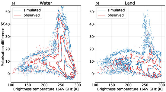
Figure 4.
The polarisation differences (166V − 166H) as a function of TB 166V GHz for observed (red) and simulated (blue) values for water (a) and land (b). The PDs are plotted as contours of the normalised 2D histogram. Data with a bin density of less than 10 are also shown as dots. The polarisation effects from the surface are included. The simulations and observations were from January 2009 and January 2017, respectively.
4.1.4. Polarisation Differences at 660 GHz
With the increasing interest towards sub-mm wavelengths, we also simulated the polarisation signals at 660 GHz using U(1, 1.4) (Figure 5). In this plot, the filtering of cases affected by the surface was not considered. The arch shape of PDs was preserved at 660 GHz and the maximum PD was around 15 K, which occurred for the TB around 190 K. The channel 660 GHz is not sensitive to the surface (weighting functions peak in the upper troposphere); hence, the high PDs from the surface were missing. Similar results were also observed by Gong and Wu [19] from the Compact Scanning Sub-millimetre-wave Imaging Radiometer (CoSSIR) 640 GHz measurements. Their observations were mainly around the Pacific Ocean near Central America and the maximum amplitude of PDs was observed to be 10 K.
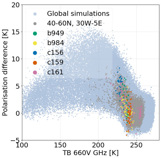
Figure 5.
The scatter plot showing the PD vs. TB at 660 GHz. The light blue dots are near-global simulations; the grey dots denote simulations in 40°N–60°N/30°W–5°E. The five alphanumeric codes depict observations from the five flight campaigns described by Fox [61].
We also compared our simulations to observations from five flight campaigns conducted by the Facility for Airborne Atmospheric Measurements (FAAM) BAe-146 research aircraft. These flights flew around the UK during March 2016, March 2019 and October 2016. More details about these flights are described in Table 2 of Fox [61]. The observations were averaged at 6 km along-track to match the GMI resolution. Out of the five flights shown, C161 had the highest observed IWPs that corresponded to PDs greater than 5 K. A part of this flight had clear-sky conditions, reflected by the cluster of observations around 260 K. Most of the observations made by flight C159 were for low altitude clouds [61,62] and had relatively small brightness temperature depressions for clear sky. The negative PDs were most likely due to noise. B984 also observed similar values during the initial and final legs of the flight.
4.2. Snow Emissivity Model
For water bodies, the TESSEM model is valid to sufficiently high frequencies, but for other surface types, no ready models are at hand for the estimates of land, sea ice and snow emissivity. The climatology-based TELSEM has an updated version, TELSEM2 [63], which provides an emissivity database for land, sea ice and snow surface types above 85 GHz. However, the snow and sea ice emissivity estimates are empirical approximations in the latter. For example, continental snow emissivity values are assumed to be constant for frequencies above 85 GHz. The sea ice emissivities are parametrised up to 183 GHz using emissivities derived from the Special Sensor Microwave/Imager/Sounder (SSMIS) [64], but only for new ice and first-year sea ice. Multi-year ice emissivities are assumed to be constant for frequencies above 85 GHz. On the other hand, Hewison et al. [65] analysed data from aircraft campaigns and showed that emissivity at 183 GHz is higher than at 157 GHz for dry snow and sea ice surface types. In another study, Harlow and Essery [66] studied the variability of snow emissivity over different snow packs. They observed that the snow emissivities increase monotonically with increasing frequency for stratified snow. However, for fresh snow, the emissivity estimates follow a decreasing trend.
Based on the observations from these studies, we developed an empirical snow emissivity model for frequencies between 150 GHz and 190 GHz. This model produces a random estimate of the snow emissivity from a standard normal distribution that depicts valid emissivity values. It was not important to know the exact snow emissivity at a given time and position, but the distributions of simulated emissivities should follow the reality. The basic idea was to find a set of emissivity estimates that simultaneously produce the radiance closest to the measurements. This empirical model was fine-tuned by comparing the observed and forward-modelled TBs. The final version used in this study is described below.
When represents the emissivities for 193 GHz and 159 GHz, respectively, then:
where represents the standard normal distribution with mean and standard deviation . The differences between the H and V polarisations for both frequencies were approximated through a uniform random distribution.
where represents a uniform distribution between a and b. In this study, snow cover over both land and sea ice was treated identically.
Polarisation Differences over Snow Covered Surfaces
Figure 6 shows the comparison of TB-PD distribution at 166 GHz over snow covered land and sea ice surface types. The simulations only included snow covered sea ice, but the observations made no distinction between snow covered sea ice and pure sea ice. Further, cases classified as under the sea ice–water boundary and snow–land boundary were also included. The distribution of PDs was the combined effect of signatures from the surface and hydrometeor impact; no filtering was applied. However, the hydrometeor impact was expected to be small as high latitude winters are primarily associated with a dry atmosphere.
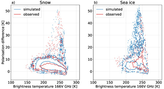
Figure 6.
The same as in Figure 4, but for snow covered land (a) and sea ice (b).
For snow cover, the PDs consisted of a distinct arch-type distribution with maximum PDs of around 10 K and an arm composed of very high PDs. In the arch region, the match between the observed and simulated PDs was relatively high, indicating that the snow emissivity that was estimated by the empirical model could replicate the observations. However, these signals could also overlap with the PDs observed from ice hydrometeor scattering. Without any additional information, it would not be trivial to separate one type of signal from the other. On the other hand, the observations had a higher spread and larger magnitudes than the simulations along the arm. The maximum observed PD along the arm was around 50 K, but the simulations could only reach up to 30 K. The very high PDs were suggestive of surface effects from mixed surface types. An analysis of these observations showed that most of these cases lay close to the water and could potentially be affected by misclassification.
For sea ice, the structure of PDs was only slightly different from snow cover. Here, the flat arch region was narrower and the concentration of observations along the arm was denser than for snow covered land. The PDs along the arch region originated from snow covered sea ice, while the higher PDs along the arm arose from a sea ice and water mixture. The differences in the radiometric responses of open water and sea ice led to varying surface emissivities over mixed surface types. Since the emissivity of water is much higher than sea ice, satellite footprints with lower sea ice fractions have higher emissivity than areas with larger sea ice fractions. A detailed description of the distribution of the sea ice and water mixture inside the footprint is required to model these emissivities correctly.
4.3. Comparison of Simulations and Observations
4.3.1. TB Distribution and IWP
This section describes the distributions of the simulated TBs for all four high-frequency channels of GMI. The simulated values were based on random CloudSat profiles; thus, only a statistical comparison to the observations was made. As mentioned, it was not necessary for the simulations to be collocated with the GMI observations in space and time, but a similar variability between the two was expected.
Figure 7 shows the distribution of the simulated and observed TBs for the four channels and the two databases that were based on large plate aggregate (Section 3.2). For all four channels, the peak of the distributions corresponded to the clear-sky scenarios, while the coldest TBs were associated with deep convective systems. For clear-sky cases, both the TRO and aARO databases agreed well with GMI. However, over the colder part of the TBs, neither of the two databases could reproduce the exact distribution. The forward simulations put more cases with low TBs. The simulations had a high occurrence frequency for all channels in the intermediate region (between 170 K and 250 K). Analysing the distributions according to surface type and latitudinal extent revealed that the mismatch was removed when TBs belonging to snow cover were omitted (data not shown). This could be due to the forward simulations having a larger representation of snow on the ground cases than GMI. Since snow cover is a variable quantity, comparing data from different years can introduce such artefacts.
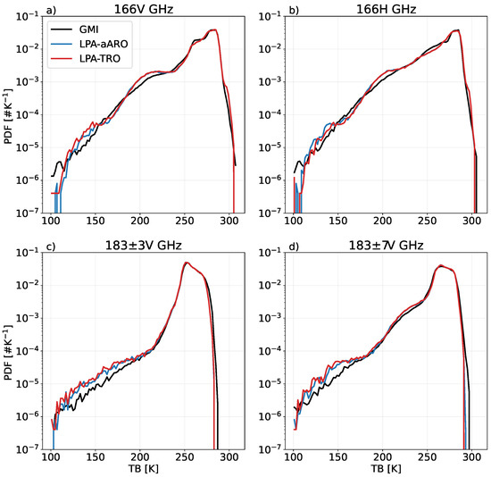
Figure 7.
(a–d) The distribution of TBs for all high-frequency channels of GMI. The simulations (from January 2009) were based on large plate aggregate. The black curve represents the GMI observations (from January 2017).
Including aARO had a small impact on the occurrence frequency of colder TBs. At all V polarised channels, simulations with aARO exhibited warmer TBs compared to the simulations for TRO. The opposite effect was seen for the H polarised channel, 166H GHz, where the aARO led to colder TBs. Similar results using the Evans snow aggregate are described in Appendix A.
4.3.2. IWP Distributions
For ML retrieval to work efficiently, the training data should reflect realistic scenarios as closely as possible. In this study, we dd not use any collocated datasets and the IWPs corresponding to the synthetic scenes were calculated by inverting the CloudSat reflectivities. This is explained in detail in Ekelund et al. [41], but here, we provide a comparison of the inverted IWPs and the IWPs provided by the raDAR/liDAR cloud product [67] (DARDAR) in Figure 8. Although, DARDAR may provide the best estimate of IWP, it is not free from uncertainties. The retrieval uncertainty in Cloudsat IWC has been quantified at around ±40% in [68,69]. We assumed the same error estimate for the DARDAR product. On the other hand, the uncertainties in inversions are dominated by the forward-model assumptions. Ekelund et al. [41] have shown that dbZ inversions are quite sensitive to microphysical assumptions. They reported that the retrieved IWC fields can differ by over one order of magnitude between different particle models.
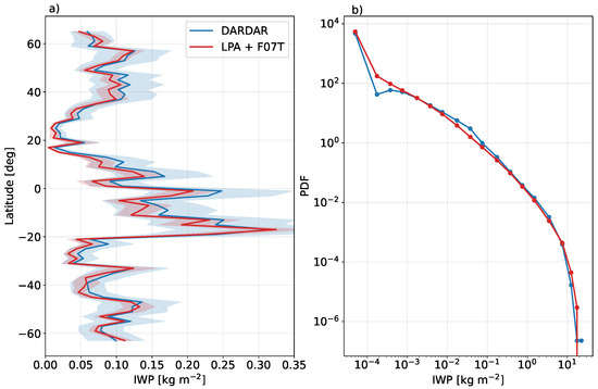
Figure 8.
A comparison of the (a) the zonal means and (b) PDF of the IWPs from the DARDAR product and the IWP obtained by inverting CloudSat reflectivities. The blue shaded region corresponds to the ±40% uncertainty in the DARDAR IWP (see text), while the red shaded region represents the one standard deviation around the mean of the simulations, which was calculated by random sampling with replacement (bootstrapping). The particle model for simulations (red) was large plate aggregate (LPA) + F07T. The data were from January 2009.
Overall, the radar inversions agreed fairly well with the DARDAR IWPs, but the magnitude of the zonal means that was obtained from the database could be up to 16% smaller than from the DARDAR. The greatest differences arose due to the different particle models used by the DARDAR product and our forward simulations. Additionally, DARDAR retrievals include lidar measurements that are sensitive to thin ice clouds. The lack of such measurements in our inversions led to lower IWCs at high altitudes (where thin cirrus clouds are abundant) compared to DARDAR.
4.4. IWP Retrievals
4.4.1. Retrieval Experiments
Two retrievals were performed, both with and without orientation. A separate QRNN was trained for each of the two databases, i.e., LPA-aARO and LPA-TRO (Section 3.2). The basic construction of both trainings was identical, but each was based on the input database. All four high-frequency channels of GMI were included in the input. The details of the QRNN configuration, ancillary data and data augmentation are described in Appendix B.
4.4.2. Basic Retrieval Performance
The retrievals from a test dataset were compared to the true state vectors to evaluate the retrieval performance of the QRNN. The IWP retrievals from QRNN are henceforth referred to as Q-IWP (QRNN-Ice Water Path). The test dataset was part of the LPA-aARO database, but was not revealed to the network during training. It provided a way to check the model accuracy against the data that were not used in the training procedure. This was an idealised retrieval where the training and test datasets had the same underlying a priori distributions. The expectation value was taken as the point estimate (Section 3.4) and is hereafter also referred to as “retrieved IWP”. Further, the true state vectors from the test dataset are referred to as “reference” in the following figures and the text. The distribution of the predicted posterior distribution was also analysed by selecting ten random samples for each case from the predicted distribution.
Figure 9a shows the normalised distributions of the true and retrieved state vectors. For low IWPs (<0.01 kg m), the occurrence frequency of retrieved IWPs was higher, while the cases with very high IWPs (>10 kg m) occurred less frequently. For the intermediate IWP range, the posterior distribution and retrieved IWPs overlapped, indicating that the retrievals were sharper and better calibrated. However, for the very low IWPs, the retrieved IWPs had a poor fit to the reference. This indicates poor calibration for low IWPs. This was not unexpected as the passive microwave instruments in the millimetre (mm) range are sensitive to IWPs greater than ∼0.2 kg m (See Figure 1 of [70]). Overall, Q-IWP overestimated the low IWP values (thin ice clouds) and slightly underestimated the larger IWPs (thick ice clouds). However, the posterior distribution predicted by Q-IWP was of high interest here. It captured the entire reference distribution, except the very high values above 10 kg m. A high degree of match between the posterior and reference distribution confirmed that Q-IWP could combine the information provided a priori and the input data to output a well-defined posterior. Figure 9c shows the deviation of the retrieved IWP from the reference. It also shows the predicted error, i.e., the deviation of the random samples from the reference. The underestimation of cases with high IWP caused the error distributions to be asymmetric; however, the distribution of predicted errors had a lower skewness. The low accuracy of the high values was likely due to the under-representation of such cases in the a priori dataset. Any ML model is expected to learn about data from the a priori distribution and input data. Any missing information is always conditioned a priori. Ideally, a real inversion database should cover a larger period; however, we only covered one month. Thus, complete information could not always be expected.
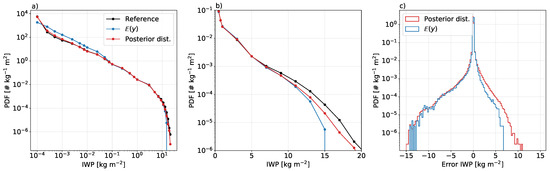
Figure 9.
(a) The PDF of the retrieved and reference (test data) IWPs. The distribution of the random samples drawn from the posterior distribution is shown in red. The point estimates of IWP retrieval are represented by the expectation value (blue). (b) Same as (a), but zoomed in on the higher IWPs. (c) The error distribution. The data were from January 2009.
4.4.3. Impact of Oriented Hydrometeors
A comparison of the IWP retrievals from the QRNN models that were trained on aARO- and TRO-based databases was carried out to examine the impact of oriented hydrometeors. Both QRNN models retrieved IWPs from an identical test dataset that was based on aARO. The reason for using the same dataset for both retrievals was so that the simulations, including aARO, better represented reality. A poorer performance was expected for the TRO-based retrieval as it neglected hydrometeor orientation. However, the comparison of these two retrievals (aARO- and TRO-based) helped us to quantify the impact of polarised signals on retrieval accuracy.
Figure 10 shows the error statistics for retrievals based on the TRO and aARO databases. The retrieved data were binned according to . For up to 1.09, both retrieval sets produced similar accuracies, but as increased, differences showed up. For between 1.1 and 1.23, the bias in retrievals with the TRO was lower than aARO, but Mean Absolute Error (MAE) showed that ARO retrievals had a better accuracy. At the same time, Root Mean Squared Difference (RMSD) remained unchanged. However, for , the differences between the two retrievals were quite prominent. TRO retrievals had a positive bias, showing up as elevated MAE and RMSD. For , the RMSD decreased by almost 50%. This was not unexpected as reproduces the largest PDs, which TRO cannot represent. While the MAE and RMSD showed a clear trend in improving accuracy with aARO, the fluctuating trend in bias needed investigation. Thus, we analysed the zonal averages for the aARO and TRO retrievals (Figure 11). Over the tropics, the TRO-based retrievals had a higher magnitude than the reference. Between the equator and 30°S, which follows the Intertropical Convergence Zone (ITCZ), the TRO retrievals were 16% higher than the reference, while the aARO retrievals showed an excellent match to the reference. In this region, the bias in the aARO and TRO retrievals was −0.003 kg m and 0.025 kg m, respectively. At higher latitudes, the differences between the two retrievals were small. In the northern hemisphere (north of 30° N), the retrievals belonged to a winter scenario. Here, the zonal averages of both retrievals were quite similar, but the TRO retrievals had a lower bias (−0.006 kg m) compared to the aARO retrievals (−0.009 kg m). However, in the southern hemisphere, the low accuracy of TRO with respect to the reference was evident between 30° and 45°S, but at high latitudes, both the TRO- and aARO-based retrievals had quite similar average values and both were able to match the highest observed IWPs.
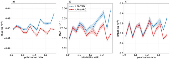
Figure 10.
The statistics for (a) bias, (b) mean absolute error (MAE) and (c) root mean square difference (RMSD) show the accuracy of the retrieved IWPs (from test data) and were binned according to the polarisation ratio () into bins with a width of 0.03 each. The shaded region in all plots represents the one standard deviation of around the mean, quantified by random sampling with replacement (bootstrapping). The simulations were based on the large plate aggregate.
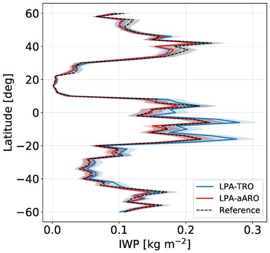
Figure 11.
The zonal means of the IWP retrievals based on the LPA-aARO and LPA-TRO databases. The reference (test data) is shown in black. For all three datasets, the shaded region represents the one standard deviation around the mean, calculated by random sampling with replacement (bootstrapping).
Further, we analysed the performance of the IWP retrievals according to surface type. Figure 12 shows the bias and MAE values for the two retrievals. Over water, the total bias between the reference and retrievals was 0.006 kg m, which indicates that with aARO, the retrievals had a lower magnitude. On the other hand, the lower MAE values indicate better accuracy. The MAE for the entire dataset decreased from 0.044 to 0.037 kg m with aARO. A similar performance was observed over land, but TRO produced a higher positive bias (0.012 kg m) and the accuracy reduced by 26%. For other surface types, varying accuracy was observed. Both retrievals had a comparable performance for snow covered land, but the MAE was almost 60% of the mean IWP. The random uncertainty was also higher. This could be due to an increased frequency of both false positives and negatives, i.e., the retrieval of non-zero IWPs for a clear case and vice versa. Most false negatives occurred for water and snow-cover surface types and towards the warmer TBs (less than 190 K at 166V GHz). For the former, such cases were mostly concentrated at 275 K and low values of PD. However, for the snow surface type, missed retrievals were spread out over the entire range of TBs. Around 25% of false positive cases also belong to snow-cover. For sea ice, both retrievals were larger than the reference and the average bias in the retrievals assuming TRO was twice as high as aARO.
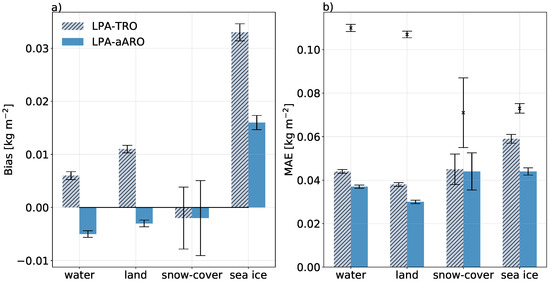
Figure 12.
The (a) bias and (b) mean absolute error (MAE) of the retrieved IWPs (test data) using the aARO- and TRO-based databases for different surface types. The black crosses in (b) represent the mean of the reference IWPs. The error bars mark the one standard deviation around the mean, calculated by random sampling with replacement (bootstrapping).
Analysing the accuracy over different IWP ranges (table not shown) revealed that the overall retrieval performance was driven by the retrievals with IWP > 0.5 kg m over water. Further, we also observed that for very low IWPs (< 0.01 kg m), the performance of both retrievals was almost identical. The bias and MAE had similar values in this range, which reflected the overestimation of the very small values. In the intermediate range (0.01 kg m < IWP < 0.5 kg m), both retrievals were lower in magnitude than the reference, but the LPA-aARO was closer to the reference.
4.5. Retrieval Applied to GMI Measurements
The performance of the retrieval algorithm on real measurements was analysed using GMI data from January 2017. In the absence of a reference for benchmarking these results, we analysed an example scene for qualitative analysis. Figure 13 shows a convection system in the tropical Indian Ocean and the corresponding TBs at 166V GHz, PDs and the retrieved IWPs using the LPA-aARO database. The retrieved IWPs followed the pattern of convective activity. The maximum IWPs were around the convection centres and decreased monotonically as the distance from the centre increased. The maximum retrieved IWP in this region was greater than 10 kg m. However, when the hydrometeor orientation was neglected, the retrievals were higher in magnitude, as seen by the positive relative differences. The IWPs along the convective activity could be around 20% higher. While we did not have any reference value to compare to, these results conformed with the trend observed in the test retrievals (Section 4.4.3).
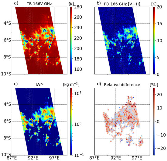
Figure 13.
(a–d) An example convection system observed by GMI on 15 January 2017. The top two panels show the observed TBs at 166V GHz and the PD between the dual-polarised channels (166V − 166H). The bottom left-hand panel shows the retrieved IWPs when oriented hydrometeors were considered, while the right-hand panel shows the relative differences from the IWP retrievals when the orientation was neglected. The relative differences for clear-sky regions (IWP < 0.01 kg m) were masked.
While this example can demonstrate how the two retrievals differed, it is not sufficient to describe the global differences. Figure 14 quantifies the average IWPs from both TRO and aARO retrievals for different PDs bins. IWPs with a magnitude less than 0.01 kg m were not included in these statistics in order to exclude clear-sky cases. For PDs < 10 K, both retrievals were quite similar and the differences were of the order of 1–2%. These could also be due to retrieval uncertainties. However, as PD increased, neglecting orientation led to around 20% higher retrievals. For land and water, the maximum differences were 30% and 25%, respectively, and they occurred for PDs around 14 K. The differences between the two retrievals for snow covered land and sea ice regions were small for PDs up to 10 K PD. However, at higher PDs, the two retrievals began to diverge. Such cases were few and, as shown in Section 4.2, the cases with high PD mostly belonged to mixed surface types. The high errors for these regions could likely be due to misclassification.
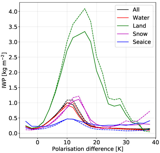
Figure 14.
The average IWPs from the two retrieval datasets, binned according to the polarisation differences. Four surface types are shown. The dotted lines denote the retrievals with the TRO assumption and the solid lines represent the retrievals with the aARO assumption.
Figure 15 shows the zonal means for Q-IWP from January 2017. The GPROF IWP product is also shown for comparison. For DARDAR, only daytime observations were available. All three datasets followed the seasonal variation of IWP, but there was a lack of agreement between the magnitudes. GPROF IWPs were too small, but Q-IWP retrievals and DARDAR had comparable magnitudes, especially over high latitudes. Over the tropics, Q-IWP had a smaller magnitude than DARDAR. This could be due to the underestimation of large IWPs. However, it is worth remembering that our retrievals had additional information in the posterior distribution. While the point estimate might fall short of reaching the observed IWPs, the observed IWP could be randomly estimated inside the fixed bounds. For example, the bounds described by the average of the 5% and 95% percentiles are highlighted in the figure.
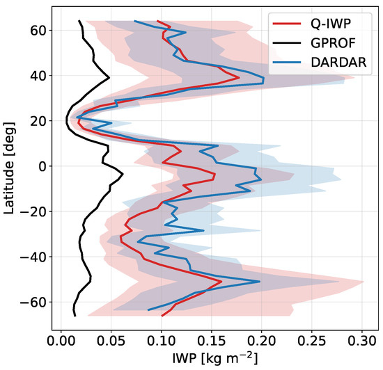
Figure 15.
The zonal means of Q-IWP, GPROF and DARDAR observations for January 2017. The blue shaded region for DARDAR corresponds to the ± 40% uncertainty, while the limits of the red shaded region are the mean of the 5% and 95% percentiles. For DARDAR, only daytime observations were available.
Figure 16 displays the gridded means for Q-IWP, GPROF and DARDAR (all from January 2017). The SPARE-ICE product (Synergistic Passive Atmospheric Retrieval Experiment-ICE [71]) is also plotted for a broader comparison. The observations from SPARE-ICE and GMI do not have a common overlap year; thus, the SPARE-ICE data were from 2013. The DARDAR data only include daytime values. All four datasets had distinctive common features, which roughly matched in location. The highest IWPs were clustered around the ITCZ, which defines the maximum tropical convective activity. The higher IWPs around 40°N and 40°S were caused by mid-latitude storms. On the other hand, the lowest IWPs regions were along the stratocumulus regions, where dry and stable air prevents the vertical development of the cloud structure. Low IWPs were also observed along the Sahara desert and the Arabian peninsula. While the general gridded distribution of the IWPs in all four datasets seemed quite similar, differences existed in magnitude and on local scales. While Q-IWP and GPROF had quite similar features over the tropics, the magnitude differed to a great extent. Further, GPROF did not retrieve IWPs over snow covered surfaces; this led to gaps over Siberia and almost zero IWPs over North America. However, in Q-IWP, retrievals were made for all surface types. Further, Q-IWP had more atmospheric ice in the storm belt than SPARE-ICE. While this was consistent with the DARDAR observations, neither could be verified as correct. Similarly, SPARE-ICE retrieved more ice over the tropics, which was consistent with DARDAR. While one type of retrieval matched well with the other in certain areas, it could not be verified as to whether one was more accurate.
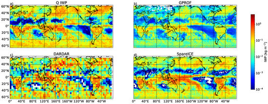
Figure 16.
(a–d) The gridded mean of the IWP observations for Q-IWP, GPROF, DARDAR and SPARE-ICE. Q-IWP, GPROF and DARDAR data were from January 2017, while SPARE-ICE data were from January 2013. DARDAR is gridded at 5° grid, while the other three datasets are gridded at 2°.
5. Discussion
5.1. Polarisation Differences
A correction scheme (Section 3.3) was implemented to replicate the polarisation signals in our database. This scheme modified the TRO extinction in V and H polarised channels by a factor to mimic the effects of ARO. Five experiments with were conducted to select the best performing . Here, denotes the TRO, i.e., there were no differences between the extinctions of the V and H polarisations. On the other hand, from 1.1 to 1.4 introduced increasing differences between V and H polarisation. For example, implied an adjustment in the extinction by 4.8%, while adjusted the extinction by 16.7%. With the TRO (), there were no differences between the extinctions of the V and H polarisations; hence, the PDs were expected to be close to zero. However, as seen in Figure 3 with , the simulated PDs were mostly concentrated around 0–3 K, but some cases with PDs of 5 K or higher were also simulated. The former cases were due to the scattering from TRO [57,72] and also due to the effect of noise, but the latter were most likely due to unfiltered surface contamination. Additionally, the effect of noise also led to negative PDs, as seen in Figure 3. Negative PDs at colder TBs could be due to vertically oriented hydrometeors [19,25], but these were not simulated in this study.
The results from experiments with showed that a constant selection of paired with one habit and size distribution could only reproduce a narrow region of PDs; however, collectively, these five experiments could generate the complete PD-TB distribution. In this study, since we accommodated only one particle model, choosing a constant constrained the PDs to a narrow range. Thus, a random selection of from a distribution between 1 and 1.4 was chosen for the large plate aggregate to induce polarisation in our modelling framework. Two distributions, a uniform and truncated normal distribution, were tested and the former was found to be slightly better performing. For the Evans snow aggregate (Appendix A), a similar analysis showed U(1, 1.5) as the best performing.
The different valid ranges of for the two habits demonstrate that polarisation signals were affected by the microphysical representation, as also pointed out by Brath et al. [13] and Barlakas et al. [14]. For instance, neither particle habit could simulate the coldest TBs, but the Evans snow aggregate also failed at simulating optically thick clouds.
5.1.1. PDs over Water and Land
In the selection of , only the PDs arising from hydrometeor impact were considered. However, PDs can also occur due to the impact of the surface. Figure 4 describes the PDs observed over water and land, which were both due to the effect of hydrometeor scattering and the impact of the surface at 166 GHz. These PDs have been conceptually described by Gong and Wu [19], Galligani et al. [20], but we also provided a brief description for completeness. The strong vertical arm consisting of PDs up to 50 K was due to the surface, while the arch region consisting of PDs up to 20 K was mostly from hydrometeor scattering. Over both land and water, the strongest PDs were observed under dry atmospheric conditions at high latitudes. In regions with high water vapour concentrations, typically in the tropics, the signal from the surface was attenuated and the PDs clustered around the bottom tip of the distribution. On the other hand, the maximum PDs in the arch region were produced by horizontally aligned hydrometeors in convective outflow regions, such as an anvil. The lowest observed PDs in this region were close to 0 K and occurred for the coldest TBs, representing the deep convection systems. In deep convection, the high turbulence causes the hydrometeors to be randomly oriented and additionally, due to a high density of hydrometeors, the multiple-scattering cancels out PDs.
5.1.2. PDs over Snow Covered Surfaces
Polarisation signals originating from scattering by snow on the ground and sea ice have often been ignored in retrieval studies due to the difficulties in estimating emissivities. These polarisation signals behave quite similarly to ice hydrometeor scattering, making it difficult to distinguish between them. As a complement to our polarisation model for aARO, we also introduced a random model to estimate the emissivities for snow covered surfaces. Despite being random estimates, the range of emissivities for snow covered regions obtained from our model was also comparable to emissivity estimates retrieved from passive microwave instruments. For instance, Munchak et al. [73] retrieved emissivities for GMI using the optimal estimation method. They defined 20 snow covered surface classes for which the emissivity estimates vary between 0.75 and 0.92 at 166 GHz. These values are quite comparable to the snow emissivity estimates from our model. Similar values were also reported by Camplani et al. [74] for snow covered surfaces.
Using these emissivity estimates, we could reproduce most of the observed PDs for snow covered land and sea ice. The PDs that could not be replicated within our set-up mostly belonged to mixed surface types. For example, the emissivity for regions with partial snow cover varied according to the snow fraction in the footprint. The case was similar for sea ice. The exact distribution of snow–land and sea ice–water boundaries inside the footprint are known to handle such cases accurately, which was unfortunately not possible with the coarse resolution of the ERA5 reanalyses.
5.1.3. PD at 660 GHz
We also extended our polarisation model to the sub-mm range by simulating the TBs at 660 GHz. Using the same selection of as at 166 GHz, the arch relationship between PD and TB at 660 GHz could be simulated, but it was difficult to judge the exact fit due to the limited amount of observations. Further, with an identical range of , the maximum simulated PDs at 166 GHz were higher than at 660 GHz. This indicates that the upper limit of might increase with increasing frequencies. This was not unexpected as at 660 GHz, the sensitivity to small oriented hydrometeors was stronger than at 166 GHz. This was also seen in Figure 1, where at low IWC, the differences in extinction at 660 GHz were more significant than at 166 GHz. Previously, Gong and Wu [19] also concluded a similar behaviour while studying the effect of aspect ratio on the bell–arch curve ( is an indirect representation of aspect ratio). While it was difficult to predict the range of that could reproduce the future observations from ICI, selecting > 1.4 was not ruled out so as to maintain a buffer zone of variability. It can be argued that with the limited observations from flight campaigns, it is not feasible to completely solve the entire variability of PDs.
5.2. TB Distributions
The limitation of simplified microphysical assumptions was also seen in the comparison of the TB histogram of GMI observations and simulations. While the overall agreement was reasonably good, the main differences existed towards the colder brightness temperatures, which reflect the deep convections systems. While both habits failed to correctly simulate deep convection, they both showed contrasting behaviours. The large plate aggregate resulted in larger TB depressions than the Evans snow aggregate (Appendix A). Ideally, the perfect agreement with GMI observations can only be achieved by assuming multiple particle habits and PSD. However, such a complex microphysical scheme would have also required additional auxiliary data to identify the cloud scenarios. This would have increased the intricacy of the retrieval and further complicated any attempts to impartially certify the impact of our scheme on the retrieval. Ekelund et al. [41] made a detailed analysis of various habit and PSD combinations. Among the different habit and PSD combinations, they found that F07T with large column aggregate produced the best fit to TB distributions. However, in this study, the choice of large plate aggregate was motivated by results from Geer [39] and Pfreundschuh et al. [62]. Both studies showed that large plate aggregate has good general performance.
5.3. Impact of Orientation on IWP Retrievals
Hydrometeor orientation has a substantial impact on retrieval accuracy. When orientation was neglected, the retrievals had a strong bias, typically in the tropical regions. The way in which both V and H polarisations affect the learning curve of the ML algorithm was hard to determine, but the results show that H-polarised channels dominated the retrievals since the extinction was stronger than in V-polarised channels.
The cases that had the largest contribution to the differences between the TRO- and aARO-based retrievals belonged to high PDs. For , the retrieval error was almost 27% higher when orientation was neglected. This was comparable to the retrieval error hypothesised by Gong and Wu [19]. These errors were mostly linked to the ice clouds in convective outflow regions, where the maximum PDs were observed. On the contrary, the retrievals were practically equivalent for small values of , i.e., when PDs were small. In reality, the PDs were a mixture of signals from both randomly and preferentially oriented hydrometeors and the overall retrieval error was only 10% larger when polarisation was neglected.
5.4. Other Factors Affecting Retrieval Performance
The retrieval algorithm presented here was based on an observation database and ML. The database quality drove the performance of the retrievals. The database was based on the inversions of CloudSat reflectivities to IWCs that were conditioned by microphysical assumptions. The assumptions had simplified microphysics, i.e., one particle habit and PSD constrained the forward-model. While this assumption provided us with good agreement with the GMI measurements, the distribution over convective systems could not be fully reproduced. This may not be much of an issue when it comes to evaluating the physical limits of the retrieval. However, this introduced errors for measurements where the a priori assumptions cannot be fulfilled for convective regions.
The retrieval of IWPs for clear-sky and thin cirrus scenarios was affected by a systematic overestimation. While such cases occurred frequently, the accuracy was limited by the sensitivity of the satellite observations on which the retrievals were based. The passive microwave instruments in the mm range were sensitive to IWPs greater than ∼200 g m (See Figure 1 of [70]). For cases with lower IWPs, the ML model only had the a priori information at its disposal. The sensitivity of QRNN to low IWP cases could only be improved by additional input information, for example, observations from the sub-mm range (sensitivity from about 10 g m).
Another factor that affected the accuracy was the bias originating from the poor representation of extreme values. IWP had a very high dynamic range and very high IWPs of the order of 10 kg m occurred occasionally. However, this can be certainly be improved by incorporating more data. This study aimed to highlight the importance of polarised observations on IWPs retrievals; thus, only a limited time analysis was provided. Extending our retrieval to other seasons and latitude ranges could help to improve the representation of extreme cases. Modelling errors associated with radiative transfer and ML can also possibly introduce uncertainties. However, they were not considered. It should also be noted that retrieval errors for measurements were expected to be larger due to instrument uncertainties that were not considered in the database.
The retrieval accuracy also showed a weak dependence on the surface type. The retrievals over water and land had a similar trend, but both retrievals (aARO and TRO) had a positive bias over sea ice. Over snow covered land, the impact of orientation was not seen. However, the extra-tropical retrievals for snow covered surfaces had poorer accuracy than at high latitudes. This could be explained by the attenuation of radiation by water vapour. Higher water vapour can attenuate radiation in the extra-tropics and reduce the impact of the surface. The TBs could appear warmer despite the presence of snow on the surface. On the other hand, the atmosphere is primarily dry for high latitude winter scenarios and the surface affected the measured TBs. The low concentrations of water vapour in the atmosphere combined with low surface temperatures could result in low TBs, which resemble TB depressions originating from cloud ice. Despite that, the retrieved IWPs did not show any significant degradation in accuracy. This indicates that the ML model could learn to effectively differentiate between the signals induced by hydrometeors and those induced by the surface. This was also true for sea ice, where hydrometeor orientation clearly had a positive impact. This was an important result as most retrieval algorithms, including GPROF, exclude snow covered surfaces. In future, additional information, such surface emissivities, could also be added to distinguish overlapping signals and improve retrievals further, especially for the extra-tropics
5.5. Retrievals with GMI Observations
Although it was difficult to perform a quantitative analysis of accuracy in the absence of reference IWP, the overall performance of Q-IWP showed a significant improvement over GPROF IWP retrievals. The Bayesian retrieval algorithm utilised by GPROF to retrieve IWP uses the same database as that used for precipitation retrievals. This a priori database was generated for hydrometeor profiles covered by GPM Dual Precipitation Radar (DPR), which is only sensitive to precipitating hydrometeors. Thus, it does not cover non-precipitating ice hydrometeors. As a consequence, the GPROF IWP estimates only reflected the lower bound for IWP and led to discrepancies when comparing IWPs from different sources [75]. Additionally, GPROF excludes snow covered regions from the retrieval, which led to data gaps over higher latitudes, particularly during the winter months. This was crucial as retrieval algorithms focusing on cloud ice, and even snowfall [76], exclude snow covered regions due to the complexity of surface types. Q-IWP managed to alleviate these limitations to a great extent.
The retrievals with GMI observations showed a clear impact of hydrometeor orientation on retrieval accuracy. However, it was impossible to quantify the total positive impact without reference observations. While the magnitude of Q-IWP were pretty comparable to DARDAR, it should be noted that the level of consensus between the various products measuring atmospheric ice was mixed [75]. The biggest underlying reason for the differences was the varying microphysical assumptions among the different products and models. The mismatch in IWP meant that DARDAR and Q-IWP values in the tropical regions were also due to different microphysics.
6. Summary and Conclusions
Dual-polarised measurements have consistently shown that ice hydrometeors are generally oriented in nature. However, in retrieval studies, ice hydrometeors have usually been assumed to have total random orientation (TRO) in order to simplify computations. In this study, the goal was to improve microphysical assumptions by incorporating the effects of polarised scattering and quantify their impact on the retrieval of ice water paths (IWPs).
In the first segment of the study, we explored a model that could incorporate the effects of polarised scattering into the basic radiative transfer without intensive computational demands. The scattering from oriented hydrometeors introduces polarisation differences (PD) between the TBs measured at vertical (V) and horizontal (H) polarisations. These PDs vary with the cloud microphysics and can affect the accuracy of retrieval algorithms that focus on cloud ice. A model to approximate the effects of azimuthally randomly oriented (aARO) hydrometeors when reproducing the observed PDs from conical scanners was introduced by Barlakas et al. [14]. They implemented the scheme in the scattering solver of the radiative transfer model for TOVS, i.e., RTTOV-SCATT, and reproduced the effect of ARO by scaling the optical properties of totally random orientation (TRO) for V and H polarisations. The scaling was quantified by a factor called the polarisation ratio (). However, their model was conditioned by the assimilation system (integrated forecast system, IFS) and the radiative transfer model (RTTOV-SCATT). This study attempted to extend their model to basic radiative transfer and use high-frequency Global Precipitation Measurement Microwave Imager (GMI) measurements to demonstrate our results. The main advantage of this method was that we could avoid the rigorous calculations required by a fully polarised vector radiative transfer, but could still reproduce the polarisation effects nearly totally. While a full radiative transfer could still be feasible for specific applications, the lack of an extensive scattering database for a variety of particle habits is an additional constraint.
We evaluated and constrained the selection of using an ARTS (Atmospheric Radiative Transfer Simulator). The choice of was conditioned by the best statistical fit between the simulations and GMI observations. To ensure that polarised scattering signatures from the surface did not affect the selection of , the surface impact was excluded while comparing the simulated and observed PDs. Further, the polarisation scheme was tested with two particle habits. The main conclusions are as follows:
- The valid values of are not limited to a constant number. To reproduce the broad range of observed polarisation signals, variability in is necessary. Comparing the forward simulations (using the large plate aggregate) to the GMI observations showed that a random selection of from a uniform distribution between 1 and 1.4 has the best performance in mimicking the full variability of observed polarisation patterns;
- The selection of is slightly sensitive to the assumed microphysics. Among the two particle habits examined, the large plate aggregate and Evans snow aggregate, it was seen that up to 1.5 could be included for the latter;
- The selection of also shows a dependence on the frequency. Using identical polarisation models and microphysical assumptions yielded higher PDs at 166 GHz than at 660 GHz. However, this was to be expected as sub-mm frequencies have a higher sensitivity to small oriented hydrometeors;
- Further, to complement the polarisation model, we also implemented an empirical model to estimate surface emissivities for snow covered regions. Emissivity estimates from the literature were used to develop this model, covering snow emissivities between 160 and 190 GHz. The comparisons to observations showed that the snow emissivity model could provide a fair representation of PDs observed over snow covered surfaces.
Based on the two main developments described above, we generated a database of synthetic scenarios utilising CloudSat reflectivities. By conducting a comprehensive statistical comparison of the simulations and the observations, we showed that even with the simplified microphysical assumptions of only one particle habit and size distribution, the simulation database performed well with the measured TBs distributions. Further, the inversions of CloudSat reflectivities to ice water content (IWC) were roughly of the order of the IWC measured by DARDAR. Most differences were seen in the tropics, where the inversions were smaller in magnitude than DARDAR.
In the second segment of the study, we examined the role of preferentially oriented hydrometeors in the retrieval accuracy of the integrated amount of cloud ice (IWP). A machine learning algorithm was used to retrieve the IWP and a detailed analysis of the accuracy was made using test simulations. The main conclusions are as follows:
- Even with the limited simulations in the database (1 month), it could be seen that including the orientation had a significant impact on the accuracy of IWP retrievals. Neglecting orientation introduced a large positive bias in the tropics with respect to the reference test data;
- A comparison of the retrievals based on the TRO and aARO assumptions showed that the most significant differences in retrieval accuracy occurred for cases with the highest polarisation differences. Neglecting orientation degraded the retrieval accuracy by almost 27% for PD > 10 K, while for PDs of the order of few kelvins, no significant differences were observed;
- The retrievals with GMI observations were analysed qualitatively. While it was difficult to assess the precision of the retrievals with GMI observations, a significant highlight was the improved performance with respect to GPROF (Goddard profiling algorithm) IWP retrievals. A crucial aspect was the retrieval of IWP over snow covered regions, which GPROF and other snow retrieval algorithms do not cover.
While this study mainly focused on including ice hydrometeor orientation in radiative transfer, it also demonstrated that orientation should not be neglected in retrieval studies. This becomes even more important for the upcoming Ice Cloud Imager (ICI) mission, where sub-millimetre (sub-mm) wavelengths will offer increased sensitivity to smaller ice hydrometeors. The simulation results with 660 GHz were also promising in this direction and reinforced the advantages of our polarisation model. However, the limitation to conical scanners should not be forgotten and similar work needs to be performed for cross-track scanning instruments.
Author Contributions
The study was conceptualised by P.E., V.B. and I.K. The analysis, validation and visualisation of the results were performed by I.K. with input from V.B. and P.E. The QRNN package was made available by S.P. The flight campaign data were provided by S.F. The original draft was written by I.K. with contributions from all authors. All authors contributed to the study with discussions and feedback. All authors have read and agreed to the published version of the manuscript.
Funding
The study was funded by Swedish National Space Agency grants 154/19 and 166/18. VB is supported by EUMETSAT Fellowship Programme.
Institutional Review Board Statement
Not Applicable.
Informed Consent Statement
Not Applicable.
Data Availability Statement
The data used in the analysis presented here can be made available on request.
Acknowledgments
The authors would like to acknowledge the contribution of all individuals behind the open-source software that was used (ARTS, Python, PyTorch, Numpy and Matplotlib).
Conflicts of Interest
The authors declare no conflict of interest.
Appendix A. Estimation of ρ for Evans Snow Aggregate and Comparison with Observations
Figure A1 shows the simulated PDs as a function of TB at 166V GHz for the Evans snow aggregate overlaid on the observed PDs. It is similar to Figure 3, except both water and land surface types are shown together. Compared to Figure 3, the polarisation ratio followed quite similar behaviour.

Figure A1.
The polarisation differences (166V − 166H) as a function of brightness temperatures at 166V GHz (PD-TB relationship) over water and land. The GMI observations are shown in dark grey, while the other colours represent the simulations for the different values of . The three overlaid lines represent the 5th, 50th and 95th percentiles of the observed polarisation differences for each TB interval. The simulations were based on the Evans snow aggregate. The data affected by the surface were filtered out (see text). The simulations were from January 2009 and the observations were from January 2017.

Further, the TB distributions for the four channels of GMI are displayed in Figure A2. For all four frequencies, as seen above, the Evans snow aggregate failed to simulate the coldest TBs. Still, interestingly, the mismatch between simulations and observations in the intermediate zone was smaller than that observed with the large plate aggregate. This is a significant result, reinforcing the fact that better agreements with observations are achievable by more advanced microphysical schemes covering a mixture of particle habits.

Figure A2.
(a,b) The distribution of TBs for all high-frequency channels of GMI. The black curve represents the GMI measurements. The simulations were based on the Evans snow aggregate.
Figure A2.
(a,b) The distribution of TBs for all high-frequency channels of GMI. The black curve represents the GMI measurements. The simulations were based on the Evans snow aggregate.

Appendix B. QRNN Configuration and Inputs
Several factors were crucial for implementing an optimal QRNN for the current application. The QRNN architecture that was considered for this application is described as follows:
- The QRNN predicts the posterior distribution in terms of quantiles. The quantiles are user-defined and high-resolution quantile fractions are allowed. For this study, we selected 51 equally spaced quantile fractions between 1% and 99%;
- We selected the multiple hyper-parameters, such as the number of hidden layers, layer widths and batch size, by comparing network performance over a fixed set of values. Through this iterative approach, the network architecture with the lowest mean quantile loss was chosen for all QRNN training that was presented in this study. Finally, a neural network with five hidden layers and 256 neurons in each layer was selected. The batch size was fixed at 256;
- The update to the network parameters was made with a Stochastic Gradient Descent (SGD) optimiser and cosine annealing as the learning rate scheduler. We started with an initial learning rate of 0.01 and trained for 50 epochs, then the learning rate was reduced to 0.001 and trained for a further 50 epochs. Finally, the learning rate was reduced to 0.0001 and the model was trained for 100 epochs. Using a modified learning scheduler, such as this, produced better calibration than using only one kind of adaptive learning rate.
While it was important to set up an optimal neural network architecture, finding the best combination of input variables was also crucial. Efficient retrieval performance requires the best combination of training architecture and input data. The details about the training data are as follows:
- The input vector space consisted of TBs from the four high-frequency channels of GMI, i.e., 166V GHz, 166H GHz, 183V ± 3 GHz and 183V ± 7 GHz. We also included 2 m temperature, water vapour path, surface elevation and surface type as additional inputs to identify the environmental conditions. Seven surface types were considered: water, land, snow, sea ice, coastlines, snow–land boundary and sea ice–water boundary. We classified snow–water boundary data under snow during the training as GMI did not classify these types separately;
- The IWP had a very high dynamic range. A large majority of cases had very small or zero IWPs, but values as large at 25 kg m also existed. Thus, to facilitate the optimal use of data in the neural network, a log-linear transformation was applied, i.e., all IWPs less than 1.0 kg m were transformed into natural logarithmic spaces while the other IWPs remained unchanged. Additionally, all cases with IWPs less than 10 were replaced by a small random number from the interval (10, 10);
- To avoid over-fitting an ML training model, data augmentation is often used to increase the variability in the data by adding noise. Random noise was added to TB in each training cycle and epoch for our model. The noise was added according to the NET;
- A small randomisation of the surface types was also included to take account of misclassification in the database. The comparison of the simulations and observations showed that GPROF surface classification could be wrong, particularly in regions with mixed surface types. Thus, to enhance the robustness of the ML model to these perturbations, the surface type of 1% of the data were randomly shuffled at each epoch.
References
- Stephens, G.L.; Kummerow, C.D. The remote sensing of clouds and precipitation from space: A review. J. Atmos. Sci. 2007, 64, 3742–3765. [Google Scholar] [CrossRef]
- O’Dell, C.W.; Wentz, F.J.; Bennartz, R. Cloud liquid water path from satellite-based passive microwave observations: A new climatology over the global oceans. J. Clim. 2008, 21, 1721–1739. [Google Scholar] [CrossRef]
- Greenwald, T.J.; Stephens, G.L.; Vonder Haar, T.H.; Jackson, D.L. A physical retrieval of cloud liquid water over the global oceans using Special Sensor Microwave/Imager (SSM/I) observations. J. Geophys. Res. Atmos. 1993, 98, 18471–18488. [Google Scholar] [CrossRef]
- Weng, F.; Grody, N.C. Retrieval of cloud liquid water using the special sensor microwave imager (SSM/I). J. Geophys. Res. Atmos. 1994, 99, 25535–25551. [Google Scholar] [CrossRef]
- Weng, F.; Grody, N.C. Retrieval of ice cloud parameters using a microwave imaging radiometer. J. Atmos. Sci. 2000, 57, 1069–1081. [Google Scholar] [CrossRef]
- Evans, K.; Wang, J.; O’C Starr, D.; Heymsfield, G.; Li, L.; Tian, L.; Lawson, R.; Heymsfield, A.; Bansemer, A. Ice hydrometeor profile retrieval algorithm for high-frequency microwave radiometers: Application to the CoSSIR instrument during TC4. Atmos. Meas. Tech. 2012, 5, 2277–2306. [Google Scholar] [CrossRef]
- Gong, J.; Wu, D.L. CloudSat-constrained cloud ice water path and cloud top height retrievals from MHS 157 and 183.3 GHz radiances. Atmos. Meas. Tech. 2014, 7, 1873–1890. [Google Scholar] [CrossRef][Green Version]
- Geer, A.J.; Lonitz, K.; Weston, P.; Kazumori, M.; Okamoto, K.; Zhu, Y.; Liu, E.H.; Collard, A.; Bell, W.; Migliorini, S.; et al. All-sky satellite data assimilation at operational weather forecasting centres. Q. J. R. Meteorol. Soc. 2018, 144, 1191–1217. [Google Scholar] [CrossRef]
- Evans, K.F.; Stephens, G.L. Microwave radiative transfer through clouds composed of realistically shaped ice crystals. Part I. Single scattering properties. J. Atmos. Sci. 1995, 52, 2041–2057. [Google Scholar] [CrossRef]
- Evans, K.F.; Stephens, G.L. Microwave radiative transfer through clouds composed of realistically shaped ice crystals. Part II. Remote sensing of ice clouds. J. Atmos. Sci. 1995, 52, 2058–2072. [Google Scholar] [CrossRef]
- Czekala, H. Effects of ice particle shape and orientation on polarized microwave radiation for off-nadir problems. Geophys. Res. Lett. 1998, 25, 1669–1672. [Google Scholar] [CrossRef]
- Davis, C.; Emde, C.; Harwood, R. A 3-D polarized reversed Monte Carlo radiative transfer model for millimeter and submillimeter passive remote sensing in cloudy atmospheres. IEEE Trans. Geosci. Remote 2005, 43, 1096–1101. [Google Scholar] [CrossRef]
- Brath, M.; Ekelund, R.; Eriksson, P.; Lemke, O.; Buehler, S.A. Microwave and submillimeter wave scattering of oriented ice particles. Atmos. Meas. Tech. 2020, 13, 2309–2333. [Google Scholar] [CrossRef]
- Barlakas, V.; Geer, A.J.; Eriksson, P. Introducing hydrometeor orientation into all-sky microwave and submillimeter assimilation. Atmos. Meas. Tech. 2021, 14, 3427–3447. [Google Scholar] [CrossRef]
- Spencer, R.W.; Olson, W.S.; Rongzhang, W.; Martin, D.W.; Weinman, J.A.; Santek, D.A. Heavy thunderstorms observed over land by the Nimbus 7 scanning multichannel microwave radiometer. J. Appl. Meteorol. Clim. 1983, 22, 1041–1046. [Google Scholar] [CrossRef][Green Version]
- Prigent, C.; Pardo, J.; Mishchenko, M.; Rossow, W. Microwave polarized scattering signatures in clouds: SSM/I observations interpreted with radiative transfer simulations. J. Geophys. Res. 2001, 106, 243-28. [Google Scholar]
- Defer, E.; Galligani, V.S.; Prigent, C.; Jimenez, C. First observations of polarized scattering over ice clouds at close-to-millimeter wavelengths (157 GHz) with MADRAS on board the Megha-Tropiques mission. J. Geophys. Res. Atmos. 2014, 119, 12–301. [Google Scholar] [CrossRef]
- Xie, X.; Löhnert, U.; Kneifel, S.; Crewell, S. Snow particle orientation observed by ground-based microwave radiometry. J. Geophys. Res. Atmos. 2012, 117, D02206. [Google Scholar] [CrossRef]
- Gong, J.; Wu, D.L. Microphysical properties of frozen particles inferred from Global Precipitation Measurement (GPM) Microwave Imager (GMI) polarimetric measurements. Atmos. Chem. Phys. 2017, 17, 2741–2757. [Google Scholar] [CrossRef]
- Galligani, V.S.; Wang, D.; Corrales, P.B.; Prigent, C. A parameterization of the cloud scattering polarization signal derived from GPM observations for microwave fast radative transfer models. IEEE Trans. Geosci. Remote 2021, 59, 8968–8977. [Google Scholar] [CrossRef]
- Miao, J.; Johnsen, K.P.; Buehler, S.; Kokhanovsky, A. The potential of polarization measurements from space at mm and sub-mm wavelengths for determining cirrus cloud parameters. Atmos. Chem. Phys. 2003, 3, 39–48. [Google Scholar] [CrossRef]
- Xie, X.; Miao, J. Polarization difference due to nonrandomly oriented ice particles at millimeter/submillimeter waveband. J. Quant. Spectrosc. Radiat. Transf. 2011, 112, 1090–1098. [Google Scholar] [CrossRef]
- Coy, J.J.; Bell, A.; Yang, P.; Wu, D.L. Sensitivity analyses for the retrievals of ice cloud properties from radiometric and polarimetric measurements in sub-mm/mm and infrared Bands. J. Geophys. Res. 2020, 125, e2019JD031422. [Google Scholar] [CrossRef]
- Jiménez, C.; Buehler, S.; Rydberg, B.; Eriksson, P.; Evans, K. Performance simulations for a submillimetre-wave satellite instrument to measure cloud ice. Q. J. R. Meteorol. Soc. 2007, 133, 129–149. [Google Scholar] [CrossRef]
- Prigent, C.; Defer, E.; Pardo, J.R.; Pearl, C.; Rossow, W.B.; Pinty, J.P. Relations of polarized scattering signatures observed by the TRMM Microwave Instrument with electrical processes in cloud systems. Geophys. Res. Lett. 2005, 32, L04810. [Google Scholar] [CrossRef]
- Evans, K.; Stephens, G. A new polarized atmospheric radiative transfer model. J. Quant. Spectrosc. Radiat. Transf. 1991, 46, 413–423. [Google Scholar] [CrossRef]
- Haferman, J.L. A Polarized Multi-Dimensional Discrete-Ordinates Radiative Transfer Model for Remote Sensing Applications. Ph.D. Thesis, The University of Iowa, Iowa City, IA, USA, 1995. [Google Scholar]
- Liu, Q.; Simmer, C.; Ruprecht, E. Three-dimensional radiative transfer effects of clouds in the microwave spectral range. J. Geophys. Res. Atmos. 1996, 101, 4289–4298. [Google Scholar] [CrossRef]
- Battaglia, A.; Mantovani, S. Forward Monte Carlo computations of fully polarized microwave radiation in non-isotropic media. J. Quant. Spectrosc. Radiat. Transf. 2005, 95, 285–308. [Google Scholar] [CrossRef]
- Battaglia, A.; Davis, C.P.; Emde, C.; Simmer, C. Microwave radiative transfer intercomparison study for 3-D dichroic media. J. Quant. Spectrosc. Radiat. Transf. 2007, 105, 55–67. [Google Scholar] [CrossRef][Green Version]
- Eriksson, P.; Jamali, M.; Mendrok, J.; Buehler, S.A. On the microwave optical properties of randomly oriented ice hydrometeors. Atmos. Meas. Tech. 2015, 8, 1913–1933. [Google Scholar] [CrossRef]
- Adams, I.S.; Bettenhausen, M.H. The scattering properties of horizontally aligned snow crystals and crystal approximations at millimeter wavelengths. Radio Sci. 2012, 47, 1–15. [Google Scholar] [CrossRef]
- Eriksson, P.; Ekelund, R.; Mendrok, J.; Brath, M.; Lemke, O.; Buehler, S.A. A general database of hydrometeor single scattering properties at microwave and sub-millimetre wavelengths. Earth Syst. Sci. Data 2018, 10, 1301–1326. [Google Scholar] [CrossRef]
- Troitsky, A.; Osharin, A.; Korolev, A.; Strapp, J. Polarization of thermal microwave atmospheric radiation due to scattering by ice particles in clouds. J. Atmos. Sci. 2003, 60, 1608–1620. [Google Scholar] [CrossRef]
- Battaglia, A.; Saavedra, P.; Simmer, C.; Rose, T. Rain observations by a multifrequency dual-polarized radiometer. IEEE Geosci. Remote Sens. Lett. 2009, 6, 354–358. [Google Scholar] [CrossRef]
- Balaji, C.; Deiveegan, M.; Venkateshan, S.; Gairola, R.; Sarkar, A.; Agarwal, V. Retrieval of hydrometeors from microwave radiances with a polarized radiative transfer model. J. Earth Syst. Sci. 2010, 119, 97–115. [Google Scholar] [CrossRef][Green Version]
- Ekelund, R.; Eriksson, P.; Kahnert, M. Microwave single-scattering properties of non-spheroidal raindrops. Atmos. Meas. Tech. 2020, 13, 6933–6944. [Google Scholar] [CrossRef]
- Geer, A.J.; Bauer, P.; Lonitz, K.; Barlakas, V.; Eriksson, P.; Mendrok, J.; Doherty, A.; Hocking, J.; Chambon, P. Bulk hydrometeor optical properties for microwave and sub-millimetre radiative transfer in RTTOV-SCATT v13.0. Geosci. Model Dev. 2021, 14, 7497–7526. [Google Scholar] [CrossRef]
- Geer, A.J. Physical characteristics of frozen hydrometeors inferred with parameter estimation. Atmos. Meas. Tech. 2021, 14, 5369–5395. [Google Scholar] [CrossRef]
- Eriksson, P.; Rydberg, B.; Mattioli, V.; Thoss, A.; Accadia, C.; Klein, U.; Buehler, S.A. Towards an operational Ice Cloud Imager (ICI) retrieval product. Atmos. Meas. Tech. 2020, 13, 53–71. [Google Scholar] [CrossRef]
- Ekelund, R.; Eriksson, P.; Pfreundschuh, S. Using passive and active observations at microwave and sub-millimetre wavelengths to constrain ice particle models. Atmos. Meas. Tech. 2020, 13, 501–520. [Google Scholar] [CrossRef]
- Precipitation Processing System. NASA Global Precipitation Measurement (GPM) Microwave Imager (GMI) Level 1B (L1B) Algorithm Theoretical Basis Document (ATBD) Version 3.0; Technical Report, National Aeronautics and Space Administration Goddard Space Flight Center Code 610.2/PPS Greenbelt, Maryland 20771; NASA: Washington, DC, USA, 2016. [Google Scholar]
- Kummerow, C.D.; Randel, D.L.; Kulie, M.; Wang, N.Y.; Ferraro, R.; Munchak, S.J.; Petkovic, V. The evolution of the Goddard Profiling Algorithm to a fully parametric scheme. J. Atmos. Ocean. Technol. 2015, 32, 2265–2280. [Google Scholar] [CrossRef]
- Marchand, R.; Mace, G.G.; Ackerman, T.; Stephens, G. Hydrometeor detection using Cloudsat—An earth-orbiting 94-GHz cloud radar. J. Atmos. Ocean. Technol. 2008, 25, 519–533. [Google Scholar] [CrossRef]
- Hersbach, H.; Bell, B.; Berrisford, P.; Biavati, G.; Horányi, A.; Muñoz Sabater, J.; Nicolas, J.; Peubey, C.; Radu, R.; Rozum, I.; et al. ERA5 hourly data on single levels from 1979 to present. Copernicus Climate Change Service (C3S) Climate Data Store (CDS). ECMWF 2018, 147, 5–6. [Google Scholar] [CrossRef]
- Buehler, S.A.; Mendrok, J.; Eriksson, P.; Perrin, A.; Larsson, R.; Lemke, O. ARTS, the Atmospheric Radiative Transfer Simulator–version 2.2, the planetary toolbox edition. Geosci. Model Dev. 2018, 11, 1537–1556. [Google Scholar] [CrossRef]
- Barlakas, V.; Eriksson, P. Three dimensional radiative effects in passive millimeter/sub-millimeter all-sky observations. Remote Sens. 2020, 12, 531. [Google Scholar] [CrossRef]
- Battaglia, A.; Tanelli, S.; Kobayashi, S.; Zrnic, D.; Hogan, R.J.; Simmer, C. Multiple-scattering in radar systems: A review. J. Quant. Spectrosc. Radiat. Transf. 2010, 111, 917–947. [Google Scholar] [CrossRef]
- Aires, F.; Prigent, C.; Bernardo, F.; Jiménez, C.; Saunders, R.; Brunel, P. A Tool to Estimate Land-Surface Emissivities at Microwave frequencies (TELSEM) for use in numerical weather prediction. Q. J. R. Meteorol. Soc. 2011, 137, 690–699. [Google Scholar] [CrossRef]
- Prigent, C.; Aires, F.; Wang, D.; Fox, S.; Harlow, C. Sea-surface emissivity parametrization from microwaves to millimetre waves. Q. J. R. Meteorol. Soc. 2017, 143, 596–605. [Google Scholar] [CrossRef]
- Field, P.R.; Heymsfield, A.J.; Bansemer, A. Snow size distribution parameterization for midlatitude and tropical ice clouds. J. Atmos. Sci. 2007, 64, 4346–4365. [Google Scholar] [CrossRef]
- Marshall, J.S.; Palmer, W.M.K. The distribution of raindrops with size. J. Atmos. Sci. 1948, 5, 165–166. [Google Scholar] [CrossRef]
- Rosenkranz, P.W. Absorption of microwaves by atmospheric gases. In Atmospheric Remote Sensing by Microwave Radiometry; Janssen, M.A., Ed.; John Wiley & Sons, Inc.: Hoboken, NJ, USA, 1993; pp. 37–90. [Google Scholar]
- Ellison, W. Permittivity of pure water, at standard atmospheric pressure, over the frequency range 0–25 THz and the temperature range 0–100 °C. J. Phys. Chem. Ref. Data 2007, 36, 1–18. [Google Scholar] [CrossRef]
- Saunders, R.; Hocking, J.; Turner, E.; Rayer, P.; Rundle, D.; Brunel, P.; Vidot, J.; Roquet, P.; Matricardi, M.; Geer, A.; et al. An update on the RTTOV fast radiative transfer model (currently at version 12). Geosci. Model Dev. 2018, 11, 2717–2737. [Google Scholar] [CrossRef]
- Turner, E.; Rayer, P.; Saunders, R. AMSUTRAN: A microwave transmittance code for satellite remote sensing. J. Quant. Spectrosc. Radiat. Transf. 2019, 227, 117–129. [Google Scholar] [CrossRef]
- Emde, C.; Buehler, S.; Davis, C.; Eriksson, P.; Sreerekha, T.; Teichmann, C. A polarized discrete ordinate scattering model for simulations of limb and nadir long-wave measurements in 1-D/3-D spherical atmospheres. J. Geophys. Res. Atmos. 2004, 109. [Google Scholar] [CrossRef]
- Pfreundschuh, S.; Eriksson, P.; Duncan, D.; Rydberg, B.; Håkansson, N.; Thoss, A. A neural network approach to estimating a posteriori distributions of Bayesian retrieval problems. Atmos. Meas. Tech. 2018, 11, 4627–4643. [Google Scholar] [CrossRef]
- Pfreundschuh, S. Quantile regression neural networks on top of Keras and Pytorch. 2021; Unpublished work. [Google Scholar]
- Paszke, A.; Gross, S.; Chintala, S.; Chanan, G.; Yang, E.; DeVito, Z.; Lin, Z.; Desmaison, A.; Antiga, L.; Lerer, A. Automatic differentiation in PyTorch. In Proceedings of the NIPS-W, Long Beach, CA, USA, 9 December 2017. [Google Scholar]
- Fox, S. An evaluation of radiative transfer simulations of cloudy scenes from a numerical weather prediction model at sub-millimetre frequencies using airborne observations. Radio Sci. 2020, 12, 2758. [Google Scholar] [CrossRef]
- Pfreundschuh, S.; Fox, S.; Eriksson, P.; Duncan, D.; Buehler, S.A.; Brath, M.; Cotton, R.; Ewald, F. Synergistic radar and sub-millimeter radiometer retrievals of ice hydrometeors in mid-latitude frontal cloud systems. Atmos. Meas. Tech. 2022, 15, 677–699. [Google Scholar] [CrossRef]
- Wang, D.; Prigent, C.; Kilic, L.; Fox, S.; Harlow, C.; Jimenez, C.; Aires, F.; Grassotti, C.; Karbou, F. Surface emissivity at microwaves to millimeter waves over polar regions: Parameterization and evaluation with aircraft experiments. J. Atmos. Ocean. Technol. 2017, 34, 1039–1059. [Google Scholar] [CrossRef]
- Boukabara, S.A.; Garrett, K.; Chen, W.; Iturbide-Sanchez, F.; Grassotti, C.; Kongoli, C.; Chen, R.; Liu, Q.; Yan, B.; Weng, F.; et al. MiRS: An all-weather 1DVAR satellite data assimilation and retrieval system. IEEE Trans. Geosci. Remote 2011, 49, 3249–3272. [Google Scholar] [CrossRef]
- Hewison, T.; Selbach, N.; Heygster, G.; Taylor, J.; McGrath, A. Airborne measurements of Arctic sea ice, glacier and snow emissivity at 24-183 GHz. In Proceedings of the IEEE International Geoscience and Remote Sensing Symposium, Toronto, ON, Canada, 24–28 June 2002; Volume 5, pp. 2851–2855. [Google Scholar] [CrossRef]
- Harlow, R.C.; Essery, R. Tundra snow emissivities at MHS Frequencies: MEMLS Validation using airborne microwave data measured during CLPX-II. IEEE Geosci. Remote Sens. 2012, 50, 4262–4278. [Google Scholar] [CrossRef]
- Delanoë, J.; Hogan, R.J. A variational scheme for retrieving ice cloud properties from combined radar, lidar, and infrared radiometer. J. Geophys. Res. Atmos. 2008, 113, D07204. [Google Scholar] [CrossRef]
- Heymsfield, A.J.; Protat, A.; Bouniol, D.; Austin, R.T.; Hogan, R.J.; Delanoë, J.; Okamoto, H.; Sato, K.; van Zadelhoff, G.J.; Donovan, D.P.; et al. Testing IWC Retrieval Methods Using Radar and Ancillary Measurements with In Situ Data. J. Appl. Meteorol. Clim. 2008, 47, 135–163. [Google Scholar] [CrossRef][Green Version]
- Eliasson, S.; Buehler, S.A.; Milz, M.; Eriksson, P.; John, V.O. Assessing observed and modelled spatial distributions of ice water path using satellite data. Atmos. Chem. Phys. 2011, 11, 375–391. [Google Scholar] [CrossRef]
- Gong, J.; Wu, D.L.; Eriksson, P. The first global 883 GHz cloud ice survey: IceCube Level 1 data calibration, processing and analysis. Earth Syst. Sci. Data 2021, 13, 5369–5387. [Google Scholar] [CrossRef]
- Holl, G.; Eliasson, S.; Mendrok, J.; Buehler, S.A. SPARE-ICE: Synergistic ice water path from passive operational sensors. J. Geophys. Res. 2014, 119, 1504–1523. [Google Scholar] [CrossRef]
- Teichmann, C.; Buehler, S.A.; Emde, C. Understanding the polarization signal of spherical particles for microwave limb radiances. J. Quant. Spectrosc. Radiat. Transf. 2006, 101, 179–190. [Google Scholar] [CrossRef]
- Munchak, S.J.; Ringerud, S.; Brucker, L.; You, Y.; de Gelis, I.; Prigent, C. An active–passive microwave land surface database from GPM. IEEE Trans. Geosci. Remote 2020, 58, 6224–6242. [Google Scholar] [CrossRef]
- Camplani, A.; Casella, D.; Sanò, P.; Panegrossi, G. The Passive microwave Empirical cold Surface Classification Algorithm (PESCA): Application to GMI and ATMS. J. Hydrometeorol. 2021, 22, 1727–1744. [Google Scholar] [CrossRef]
- Duncan, D.I.; Eriksson, P. An update on global atmospheric ice estimates from satellite observations and reanalyses. Atmos. Chem. Phys. 2018, 18, 11205–11219. [Google Scholar] [CrossRef]
- Rysman, J.F.; Panegrossi, G.; Sanò, P.; Marra, A.C.; Dietrich, S.; Milani, L.; Kulie, M.S. SLALOM: An all-surface snow water path retrieval algorithm for the GPM Microwave Imager. Radio Sci. 2018, 10, 1278. [Google Scholar] [CrossRef]


Publisher’s Note: MDPI stays neutral with regard to jurisdictional claims in published maps and institutional affiliations. |
© 2022 by the authors. Licensee MDPI, Basel, Switzerland. This article is an open access article distributed under the terms and conditions of the Creative Commons Attribution (CC BY) license (https://creativecommons.org/licenses/by/4.0/).