Detecting Moving Trucks on Roads Using Sentinel-2 Data

Abstract

In most countries, freight is predominantly transported by road cargo trucks. We present a new satellite remote sensing method for detecting moving trucks on roads using Sentinel-2 data. The method exploits a temporal sensing offset of the Sentinel-2 multispectral instrument, causing spatially and spectrally distorted signatures of moving objects. A random forest classifier was trained (overall accuracy: 84%) on visual-near-infrared-spectra of 2500 globally labelled targets. Based on the classification, the target objects were extracted using a developed recursive neighbourhood search. The speed and the heading of the objects were approximated. Detections were validated by employing 350 globally labelled target boxes (mean $F_1$ score: 0.74). The lowest $F_1$ score was achieved in Kenya (0.36), the highest in Poland (0.88). Furthermore, validated at 26 traffic count stations in Germany on in sum 390 dates, the truck detections correlate spatio-temporally with station figures (Pearson r-value: 0.82, RMSE: 43.7). Absolute counts were underestimated on 81% of the dates. The detection performance may differ by season and road condition. Hence, the method is only suitable for approximating the relative truck traffic abundance rather than providing accurate absolute counts. However, existing road cargo monitoring methods that rely on traffic count stations or very high resolution remote sensing data have limited global availability. The proposed moving truck detection method could fill this gap, particularly where other information on road cargo traffic are sparse by employing globally and freely available Sentinel-2 data. It is inferior to the accuracy and the temporal detail of station counts, but superior in terms of spatial coverage.

1. Introduction

Road traffic as a whole is an important source of air pollutants [1,2,3,4,5]. 86% of the transcended annual EU limits for NO${}_2$ were measured at traffic stations in 2019, according to the European Environment Agency [4]. The majority of freight is transported on roads in many countries using road cargo trucks for national and international trade [6,7,8]. This produces a significant amount of emissions [9], as most road cargo trucks are still powered by fossil fuel combustion [10]. The relevance of traffic for air-polluting emissions has been shown in various countries globally [1,2,3,5]. Additionally, the role of road cargo in national and international logistics suggests using the spatio-temporal abundance of trucks as an economic proxy [11,12,13]. This nexus of economy, cargo traffic, and emissions has also been evident during the COVID-19 pandemic that is widely associated with decreased NO${}_2$ concentrations [14,15,16].

Monitoring road cargo truck traffic is thus important for depicting spatial patterns of economic performance and emissions.

A core part of road traffic observation is the detection of actual traffic by type [17]. Traditionally, this has been approached using automatic count stations, registering traffic at selected sites [18]. Some countries operate station networks, e.g., Germany [19], the United States [20] and Austria [21]. However, such intrusive monitoring techniques [22] are expensive and their operation may disrupt the traffic [17,23]. Various non-intrusive and off-roadway traffic monitoring approaches [22] have been presented, that use e.g., cameras [24], mobile phones [25] and social media data [26], and wireless sensors [22,27]. While these measurements are conducted at a high temporal resolution, the observation stations are operated sparsely and many regions lack such measurement networks at all [18,23]. Remote sensing analysis as an independent space-borne monitoring method [22] may fill these gaps with its repetitive availability, covering large areas especially where no traffic monitoring through ground devices are installed [23]. Due to the relatively small size of road vehicles mainly very high resolution (VHR) data have been used for vehicle detection [23,28,29,30,31,32,33,34,35,36,37,38,39,40,41,42,43,44,45,46,47,48,49,50]. We suggest using passive optical Sentinel-2 remote sensing data for detecting moving trucks on roads. The presented method exploits a temporal sensing offset of the Sentinel-2 multispectral instrument (MSI) [51,52,53,54,55]. Sentinel-2 data has global coverage, a regular 5-daily revisit, and mission continuity [54,56]. These are advantages compared to traffic count stations and VHR remote sensing data. With the presented method, we aim to examine and validate the detectability of moving trucks in Sentinel-2 data.

Background

The first remote sensing studies of traffic mostly used airborne systems such as zeppelins, helicopters and aircrafts [57]. Multiple optical cameras mounted on aircrafts have been utilized at selected sites for detecting vehicles and quantifying their velocities [18,58,59,60]. Yao et al. [61] detected vehicles relying on airborne laser scanning (ALS). TerraSAR-X data were also employed for vehicle detection and speed approximation [62,63]. Early approaches based on very high resolution (VHR) spaceborne data were presented e.g., by Gerhardinger et al. [23] and Hinz et al. [64]. The latter exploited the vehicle shadow as a result of time-specific sun angles. Larsen et al. [65] incorporated this property into a classification-based approach. VHR data availability have created new potentials in object-based remote sensing [66], including vehicle detection using e.g., WorldView [67,68] and Planet Labs data [28]. Pesaresi [69] made use of a sensor-internal acquisition time-lag between multispectral and panchromatic bands. An equivalent idea uses satellite video data [50,70,71,72,73]. Remote sensing night light data has been used for a general approximation of traffic density [74]. In recent years, object-detecting neural networks, in particular convolutional neural networks (CNN), have been used extensively for vehicle detection in VHR aerial and spaceborne data [29,30,31,32,33,34,35,36,37,38,39,40,41,42,43,44,45,46,47,48,49,75]. The disadvantage of most VHR systems is their irregular acquisition [60,62]. In this paper, we present a method for large moving vehicle detection using regularly acquired multispectral Sentinel data at 10 m spatial resolution. The Sentinel-2 mission is part of the Copernicus earth observation program owned by the European Commission (EC) and operated by the European Space Agency (ESA) [76]. Sentinel-2 A/B are optical satellites carrying a push-broom MSI that captures reflected solar electromagnetic radiation in 13 bands ranging from VIS, through NIR to SWIR [54,56]. Functionalities of MSI are explained e.g., by Gascon et al. [54]. MSI carries in sum 24 detector modules on two focal planes sensing the VIS-NIR and the SWIR respectively. MSI achieves a 20.6${}^{\circ }$ field-of-view enabling a 295 km swath width. On each focal plane, the 12 detector modules are organized in a staggered layout. This causes an inter-detector shift between odd and even detectors of 14–48 km along track. In addition, there is an inter-band measurement shift within each detector module causing a displacement of up to 17 km along track. These systematic effects cause a band- and pixel-specific line-of-sight (LOS) that is corrected during the ground processing of the data, using the satellite position, sampling date, and an earth model including a digital elevation model (DEM) [54]. This processing creates a multispectral registration of less than 0.3 pixels [53,54,55,56,77]. However, the procedure relies on a static land surface at the altitude of the earth model. Once either an object is moving (motion effect) and/or is situated at a different altitude (altitude parallax), geometric shifts may be apparent in the data. The described setup causes an inter-band parallax, which can be expressed as an angle and a temporal sensing offset: Each Sentinel-2 band is acquired at a slightly different time due to the sensor build geometry [55,77].

Altitude parallax and motion effects, have been exploited for object extraction from remote sensing data of sensors with a similar setup [69,78,79,80]. Experiences with Sentinel-2 in this regard are limited. Skakun et al. [55] emphasized the potential for high altitude or moving object detection with Sentinel-2 and analyzed band phase correlations of such objects. They calculated the minimum needed object speed to be 17 km/h. Frantz et al. [53] detected clouds based on the altitude parallax within the Sentinel-2 NIR bands. The displacements among the bands 7, 8 and 8A are depicted by a Cloud Displacement Index, composed of the band ratios and their spatial variance. P. and H. Heiselberg [51,52] exploited the altitude parallax and the movement effect for detecting ships and airplanes and calculated their speed based on the band displacement. The object detection was achieved by statistical thresholds, differentiating the target pixels from the background. Liu et al. [81] detected flying airplanes and computed their speed on global scale exploiting the Sentinel-2 altitude parallax and motion effects.

Extracting objects of sub-pixel size from Sentinel-2 data is outside the scope of the satellite, as it was mainly designed for analyzing land surfaces [56]. We present a method for detecting moving trucks based on the Sentinel-2-related motion effect. Road cargo trucks (British English: lorry) in the EU are usually up to 18.75 m long and 2.55 m wide [82]. In other countries they may be longer, e.g., in Australia up to 53.5 m [83]. An EU truck of maximum size covers 47.81 m${}^2$, which is about 50% of a Sentinel-2 10 m cell. However, given the elongated truck shape, the maximum covered area per pixel is 25.5 m${}^2$, which is a fourth of a pixel. A larger car of 4.8 m × 1.7 m size covers approximately 8% of a Sentinel-2 pixel. Our hypothesis was thus that the motion effect observed in Sentinel-2 data is only apparent for large moving vehicles, mainly being trucks and vehicles of similar size. Trucks are of lower size than Sentinel-2 grid cells. Therefore, detecting these objects requires a discrete L-resolution remote sensing model [84]. In this case, the targeted object is smaller than a grid cell.

This work refers to the target objects as “trucks”, while bearing in mind that other large vehicles may be captured as well, e.g., buses. The temporal sensing offset caused by the MSI inter-band parallax, along with the object movement, causes the observed object position to be band-specific, elongating the moving object. Yet, a first approach contributed to the Rapid Action on Coronavirus and EO (RACE) dashboard of EC and ESA showed the potential of Sentinel-2 data for large moving vehicle detection on roads [85,86]. The first approach was based on VIS band ratios. An object detection method is presented, extracting the whole distorted VIS signature spectrally and spatially. Object detection aims at locating and delineating all target objects in an image, which most methods do by winning contextual information in pixel windows [87], using spatial filters [88,89], background subtraction [66,90,91] or machine learning methods such as support vector machines, boosted classifiers, and neural networks [87,92,93,94,95,96,97,98,99]. CNNs have shown strong performance also in complicated tasks [95] by using a set of spatial filters targeting spectral-spatial patterns. Detecting small objects of a few pixels using CNNs can be challenging [100,101,102], which is the first reason why CNNs were not exploited in the presented work. Second, CNNs are often employed for detecting highly complex objects [87] that can barely be described by a comprehensible set of rules. The objects targeted in the presented work are shaped by a well-understood and documented physical sensor effect. The order of the target pixels must follow the band-specific temporal sensing offsets. In addition, the target objects are characterized by reflectance patterns. Accounting for these specifics, a Sentinel-2 truck object detection method was developed, combining an ML method for separating the target spectra from the background, and an object extraction method. A random forest (RF) classifier was trained to classify the target spectra of the assumed moving trucks, and the background spectra. The developed object extraction method uses, based on the RF classification probabilities, a recursive neighbourhood search intertwined with a rule set based on known parameters of the motion effect. The aim of the presented work was to develop a Sentinel-2 truck detection method that is potentially globally applicable. Therefore, the detection method relies on globally sampled training objects. Equivalently, the detection performance was evaluated globally. The method was validated with ground truth data in Germany, exploiting the dense traffic count station data availability. With this work, we aim at proving the concept and validating a Sentinel-2 moving truck object detection method that could be used in applications such as on traffic emissions, economy, regional development and planning.

2. Materials and Methods

2.1. Theoretical Basis

Moving objects are seen by Sentinel-2 once per band. When an object is changing its position within the band-specific temporal sensing offsets, it is captured at different band-specific positions [55] (Figure 1).

Flying airplanes inherit both the movement and the altitude effect and are thus seen in Sentinel-2 with two-dimensional pixel shifts (longitude and latitude) [55,81]. To avoid confusion of these effects, the movement-related offset is here referred to as the motion effect.

Unless a truck is (nearly) black, it can be reasonably assumed that it is reflective in VIS bands, as it is usually made of metal and truck tarpaulin. As the truck is moving, the reflectance of these materials is captured by Sentinel-2 band-wise at different positions [52,55]. This effect disassembles the truck object into its spectral parts, ordered in space and sensing time. Assumingly, the reflectance of these pixels deviates from its surrounding, and this deviation must always be band-specific at each position. Taking the center position of a truck at the start of the Sentinel-2 acquisition, the position captured by Sentinel-2 $Positio{n}_{band}$ is a function of the temporal sensing offset $t_{band}$ of a band and the speed v of the truck in km/h:

$$Positio{n}_{band}=v\times \frac{t_{band}}{3.6}$$

(1)

where division by 3.6 converts to meters. For instance, referring to B02 as a reference, at a speed of 80 km/h, the truck would be captured in B03 about 11 m and in B04 about 22 m distant from the position in B02. There is an apparent object size, as seen in the Sentinel-2 data, and the true object size, which is the length and width of the object on the ground. The apparent pixel position(s) per band must be a function of object speed and size where the latter is unknown. Yet, a minimum required speed can be approximated. When the aim is to fully sense an object of about 10 m length at least at three pixels (once per VIS band) at a 10 m resolution $res$, the minimum speed $v_{min}$ results from the sensing offset of B04 $t_{\mathrm{B}04}$ (1.01 s) in relation to B02:

$$v=3.6\times \frac{2\times res}{t_{\mathrm{B}04}}.$$

(2)

Multiplication of $res$ by 2 results in a two-pixel step with B03 sensed at the center pixel, multiplication by 3.6 converts to meters. The speed would be 72 km/h. However, aiming at sensing an object of 20 m length at least partly in three pixels would result in a minimum required speed of 54 km/h. The respective pixel of $Positio{n}_{band}$ is here referred to as the anomaly pixel of a certain band. In the simplest case, the truck is white and thus causes a balanced high signal in all VIS bands at their positions. In each band, the signal would then equally deviate from the background (road) at the anomaly pixel.

Figure 2 shows a visual example of the targeted VIS reflectance pattern.

2.2. Sentinel-2 Data

The Sentinel-2 MSI captures electromagnetic radiation in 13 bands in the VIS, NIR, and SWIR. The lowest center wavelength is 443 nm at band 1, the highest is 2190 nm at band 12. Three VIS bands (B02-B04) and one of the NIR bands (B08) are distributed at 10 m spatial resolution, six bands at 20 m and three at 60 m [54,56]. With two near-polar-orbiting satellites (A/B) the mission has a revisit time of approx. 5 days [56]. Atmospherically corrected, orthorectified Sentinel-2 Level 2A (L2A) data with multispectral sub-pixel registration were used [103]. The atmospherically corrected digital numbers (DNs) were divided by 10,000, yielding physical surface reflectances [54]. For training and validation, only cloud-free scenes were considered.

2.3. Open Street Map Road Data

All Sentinel-2 data were masked by road pixels employing Open Street Map (OSM) road data [104]. OSM data are sorted by keys that summarize several values. In the case of road data, the key is denoted as “highway”, which comprises 26 values, sorted by the road size and relevance. The focus was on trucks moving fast enough to be detectable, hence, only the road types “motorway”, “trunk” and “primary” were included. In this work, “motorway” is used interchangeably with highway. The “primary” and “trunk” road types are only referred to as “primary” for simplicity.

Road vectors were downloaded via the OSM Overpass Application Programming Interface (API) provided by the OSM Foundation [105]. Aiming at an aerial road mask, the road network line data were buffered spatially, yielding road polygons. Based on manual examinations a 20 m buffer for motorways was considered suitable. The lower road types were assigned 5 m less than the next-higher type. Finally, the road polygons were transformed into an OSM road mask on the Sentinel-2 grid of the respective area of interest.

2.4. Training and Validation Boxes

Rectangular bounding boxes, each delineating one assumed truck by four corner coordinates, were created in a set of Sentinel-2 training and validation tiles. Five regions in Europe and five globally distributed regions were selected for training. Equivalently, ten regions in the same parts of the world were chosen for validation (

Table A1. Sentinel-2 tiles and number (N) of labelled boxes.

	Sentinel-2 Tile ID	Country	N Training	N Validation
1	T31UEQ	France	250
2	T32UNA	Germany	250
3	T35JPM	Russia	250
4	T36VUM	Spain	250
5	T49QHF	Ukraine	250
6	T35UQR	South Africa	250
7	T30TVK	China	250
8	T49QCE	USA	250
9	T23KKQ	Brazil	250
10	T18TWK	Australia	250
11	T33TUN	Austria		35
12	T31UFS	Belgium		35
13	T34UDC	Poland		35
14	T29SND	Portugal		35
15	T35TMK	Romania		35
16	T37MCT	Kenya		35
17	T52SDE	South Korea		35
18	T12SUC	USA		35
19	T21HUB	Argentina		35
20	T60HUD	New Zealand		35
Sum			2500	-
			-	350
Share			85%	-
			-	15%

). In each training/validation area, one Sentinel-2 acquisition was obtained. The used dates range from 2019 to 2021. Training acquisition dates originate from the months January, March, April, June, July, August and October. Validation acquisitions are from January, May, July, August, September, October, November, December. The corresponding season varies depending on the hemisphere and climate zone. No systematic balancing by seasons was done. In sum, 2500 training and 350 validation boxes were derived. The labeling sub-area in each training area was defined by a Sentinel-2 L2A tile of 10,980${}^2$ pixels, masked by the OSM road mask. Only larger road types (motorway, trunk, primary) were considered. Though, information on the road type was not labelled, and was thus not balanced systematically. Bounding boxes, each covering a visible target object, were created. 250 of these boxes were retained per training scene. The procedure was similar in the validation areas, though only 35 target objects in a subset of the tile were extracted. There, the aim was to label all visible target objects for later calculating detection performance metrics. The target objects were labelled based on their visual appearance in a true color composite of B04, B03, and B02 stretched to reflectance values between 0 and 0.2. Three conditions had to be fulfilled for being labelled as a target object:

• a noticeably higher reflectance in one of the VIS bands compared to its VIS counterparts and the surrounding,
• the presence of condition (1) for each VIS band,
• condition (2) must be fulfilled in the direct neighbourhood and the correct spatial order.

The boxes were not the actual training data but spectra at positions of the three VIS anomaly pixels, denoted as blue, green, red. In each labelled box and for each target class, criterion $A_{class}$ for the classes blue, green, red was calculated to locate the training pixel within the box:

$$A_{\mathrm{blue}}={\rho }_{\mathrm{B}02}\times 10+\frac{{\rho }_{\mathrm{B}02}-{\rho }_{\mathrm{B}04}}{{\rho }_{\mathrm{B}02}+{\rho }_{\mathrm{B}04}},$$

(3)

$$A_{\mathrm{green}}={\rho }_{\mathrm{B}03}\times 10+\frac{{\rho }_{\mathrm{B}03}-{\rho }_{\mathrm{B}02}}{{\rho }_{\mathrm{B}03}+{\rho }_{\mathrm{B}02}},$$

(4)

$$A_{\mathrm{red}}={\rho }_{\mathrm{B}04}\times 10+\frac{{\rho }_{\mathrm{B}04}-{\rho }_{\mathrm{B}02}}{{\rho }_{\mathrm{B}04}+{\rho }_{\mathrm{B}02}},$$

(5)

described by the reflectance ${\rho }_{band}$ and a normalized band ratio within the VIS. In each box and for each class, the position of maximum $A_{class}$ was extracted and assigned the corresponding label, resulting in one label per class and box. Finally, as many background samples as target samples were randomly distributed outside all boxes to differentiate between target and non-target pixels [45,98,106,107,108,109]. To balance the training dataset [110] an equal number of background samples as in each class was chosen [106,111,112]. This resulted in 2500 training and 350 validation labels per class.

Vis Spectra

The mean spectra of B02, B03, B04 and B08 depict the Sentinel-2 reflectance values by class (Figure 3). Among the VIS bands, the peak reflectance corresponds to the class, e.g., the spectrum of the red class has its VIS peak at B04. The background class has overall lower reflectance values in the VIS, yet a higher peak in the NIR.

2.5. Machine Learning and Object Extraction Method

The moving truck detection method is divided into three stages: (1) ML prediction using a RF model [113], (2) object extraction, (3) object characterization (Figure 4). This combination of pixel and context information was chosen for exploiting both the spectral and the spatial characteristics of the targets. After pre-processing the Sentinel-2 data, the features for the RF prediction are built. The trained RF model is run, resulting in class probabilities and classification maps, which are the foundation of the object extraction. The resulting bounding box objects are characterized based on the motion effect parameters.

2.5.1. Random Forest Model

Random forest models [113,114,115,116] are well proven in classification and regression tasks [117], including many remote sensing applications [118]. They decide based on the majority vote of several random decision trees, which are systematically created [113]. The method is known to be insensitive to over-fitting, to be fast, to have few hyper parameters, and to provide intrinsic statistical measures such as for the generalization error and the feature importance [117,118,119]. In 2001, Breimann [113] initiated the known RF. It belongs to the ensemble learning ML methods, combining multiple classifiers for creating a more accurate prediction. Two fundamental principles are used for creating randomness. First, at each decision node of a tree, the features taken into account for a split are randomly picked [115,120]. In addition, the classification and regression trees (CART) technique is used [113]. That is, at each node, the selected features are analyzed based on the Gini index and consequently improved [117]. Second, RF builds the trees using an aggregated bootstrap, called bagging [113,117,119]. Building an individual tree can be summarized by the steps: (1) bootstrap sampling, (2) finding the best split feature, (3) creating node. A trained forest predicts new samples based on the majority vote of all trees [117].

2.5.2. Rf Feature Selection

The term $feature$ refers to the predictor variables used in the RF model. As emphasized by [121], feature selection based on expert knowledge may be suitable in some applications. For detecting larger moving objects, the full Sentinel-2 band stack has been exploited by Heiselberg [52]. However, a visual inspection (Figure 5) suggests that the reflectance pattern on roads targeted in the given case is hardly apparent in 20 m data.

Therefore, B02, B03, B04, and B08 were used exclusively. Anticipating inter-band reflectance relationships, two normalized ratios of the bands B${}_i$ (B03 and B04 respectively) and B${}_j$ (B02) were calculated, denoted as B03_B02_ratio and as B04_B02_ratio. The spectral variance was derived as reflectance_variance. As the targets are the deviations of reflectance from normal values, the mean of each band across the whole band array was subtracted from each band (

Table 1. Random forest features.

Index	Denotation	Explanation
0	B02_centered	Difference B02 from B02 mean
1	B03_centered	Difference B03 from B03 mean
2	B04_centered	Difference B04 from B04 mean
3	B08_centered	Difference B08 from B08 mean
4	B03_B02_ratio	Difference B03 vs. B02
5	B04_B02_ratio	Difference B04 vs. B02
6	reflectance_variance	Variation among B02, B03, B04

).

The seven features were checked for information duplication based on Pearson r-values.

2.5.3. Feature Statistics

Within the anomaly classes, the centered band reflectance values are characterized by a peak in the corresponding anomaly band, e.g., B02 in the blue class (Figure 6). Consequently, the band ratios are both mostly negative in the blue class, indicating that B02 exceeds its VIS counterparts, whereas in the green and red classes the band ratio of the corresponding anomaly band is high. In the background class, no reflectance peak is visible, which is also mirrored by low ratios. The features were checked for their correlations (Supplementary Figure S1).

2.5.4. Hyper Parameter Optimization

Aiming at well-working values for the most important parameters [119], random search was employed. The decision for random search was driven by its relative simplicity, as there is little guidance on method selection for hyper parameter tuning of random forests [122]. Random search tests random combinations of hyper parameter values in parameter-specific value ranges [123]. Three parameters were tested in 200 combinations:

1.

Number of trees (n_estimators): How many decision trees are created? It should normally be in the magnitude of a couple of 100 trees [119,122]. Range: 100–2000. Selected: 800.

2.

Minimum samples per split (min_samples_split): How many samples are needed for creating a new split? If this is not achieved, a leaf is created, hence it drives the size of the trees [119]. Range: 2–7. Selected: 5.

3.

Maximum depth (max_depth): How large are the trees allowed to be? This is defined by the longest path from the root node to a leaf [119,124]. Range: 10–100. Selected: 90.

The best combination of these parameters was selected based on the accuracy scores, derived as the ratio of correctly predicted samples and the number of samples [125]. Two other important parameters were selected without random search. The maximum features (max_features) specify how many features are used at each tree split [122]. Here, the common square root of the number of features was used [119]. Bootstrap was enabled (Supplementary Table S1).

2.5.5. Feature Importances

For each of the 10,000 samples obtained from the training data, the seven features were calculated, upon which the RF model was trained. The feature importance within the trained random forest was analyzed using the intrinsic Gini feature importance measure [117]. All features but B08_centered have an importance of at least 0.13. The highest is 0.2 for reflectance_variance (Supplementary Figure S1).

2.5.6. Prediction

The RF prediction creates two maps: (1) continuous class probabilities, (2) a discrete classification with class values in the range of 1 and 4 associated with the background and three target classes.

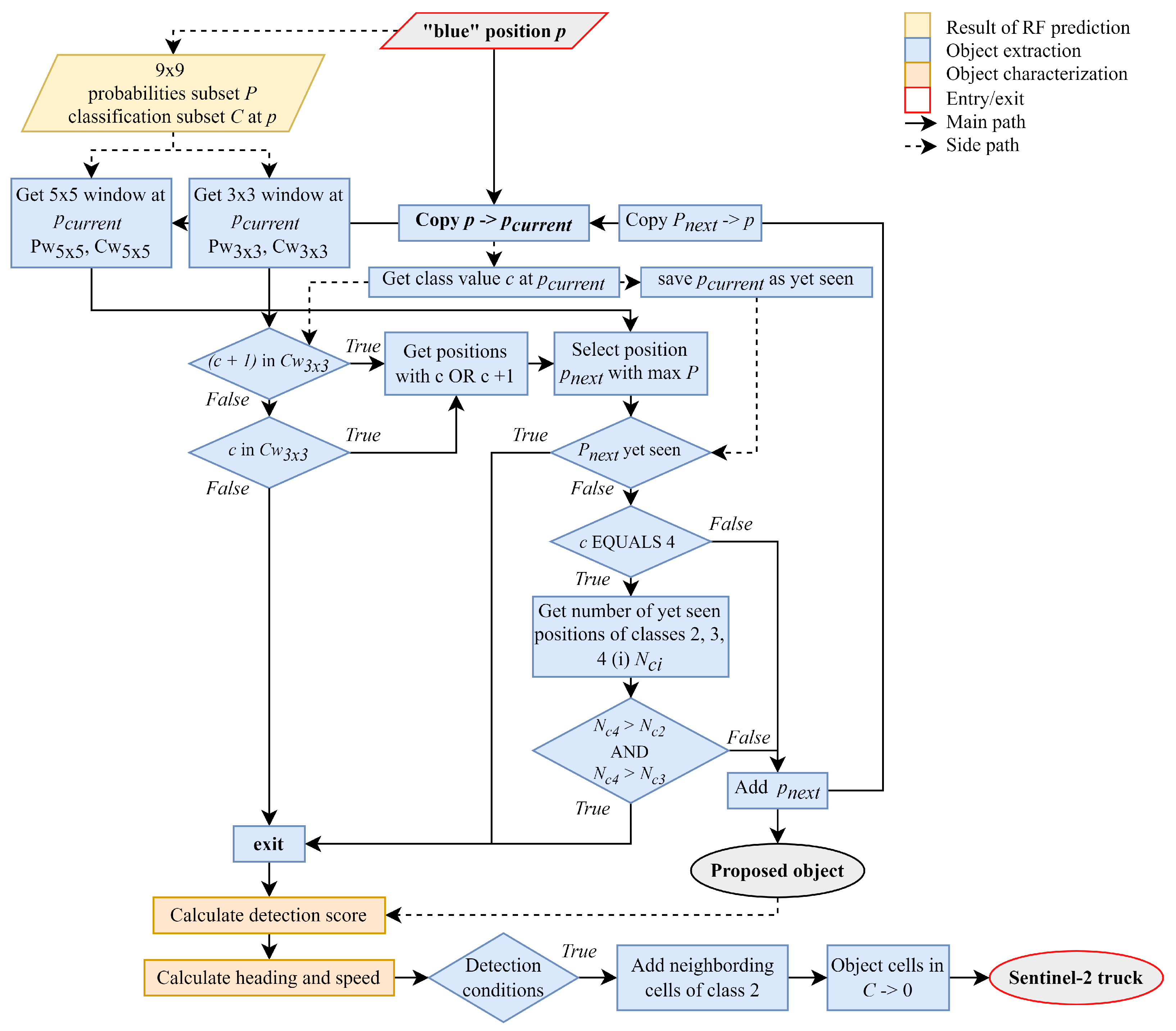
2.5.7. Object Extraction

The object extraction stage delineates the target objects based on the RF prediction. A recursive neighbourhood search approach was developed. Pixels that are classified as blue are utilized as markers for a potential target object. The object extraction iterates over all these array positions and searches a target object in the neighbourhood. Thereby, it looks for the ordered presence of pixels classified as blue, green, red (class values 2, 3, 4). Figure 7 shows the object extraction procedure, taking a blue position p with an y, x array position as the input. The possible result is an accepted object as a bounding box of four geographic coordinates.

Surrounding the y, x array position p, 9 by 9 pixel subsets of the random forest probabilities and the classification are obtained. 3 by 3 windows $C{w}_{3x3}$ of the random forest classification and probabilities are extracted. The procedure starts with the class value c = 2 (blue). It is known that within a target object this value must be neighbored by either itself or one value higher (green) (Figure 2). Similarly, this is valid for 3, which should have a 3 or 4 in its neighbourhood. However, depending on the object size apparent in the data and the classification, another 2 might be found next to a 2, but no 3. In this case, 2 is accepted. Hence, with the current c, $C{w}_{3x3}$ is first checked for $c+1$. If nothing is found, another c is searched. If again nothing is found, this may have two reasons: Either the investigated area contains no target object but just a randomly classified pixel or the object is yet completely extracted. The latter may only be the case if the current c equals 4 (red), which is the last part of the target object. Then, the current recursive process is exited and the proposed object is being characterized and checked. In case c equals 2: Assume, $c+1$ is present in the neighbourhood of p. Then, accounting for the option that there are multiple target pixels in the window, the position with maximum RF prediction probability is extracted. The resulting position is $p_{new}$. To avoid being blocked, it is checked if $p_{new}$ has yet been seen. Furthermore, if c equals 4, the extraction process finishes in case adding $p_{new}$ would result in more pixels of class 4 in the current object than of class 3 and 2, respectively. Finally, $p_{new}$ is added to the proposed object. It then becomes the new p, hence in the next recursion its neighbourhood will be investigated for target pixels. Owing to the progressive searching, pixels with value 2 are more likely to be omitted. Hence, once completed for a given input blue p, all pixels of the value 2 next to a pixel with value 2 is added to the object. Additionally, a detection score S is calculated, using the RF prediction probabilities P. At each position in the object, the maximum score among the classes 2–4 is obtained from $P_{2,3,4}$, depicted as $P_{max}$, together constituting the detection score S:

$$S=mean\left(P_{max}\right)+max\left(P_{max}\right)+mean\left(P_{2,3,4}\right),$$

(6)

between 0 and 2. The derived box has a length L and a width W. Based on the present classes, the box dimensions and probabilities, an object is accepted by fulfilling four conditions: (1) all classes 2–4 are present, (2) L > 2 or W > 2, (3) L < 6 and W < 6, (4) S > $threshold$. The values for L and W are based on the box dimensions observed in the training boxes. A set of values for the minimum score $threshold$ was examined as part of the detection performance evaluation and selected according to the highest mean F1-score.

2.5.8. Object Characterization

The detected objects inherit information from the Sentinel-2 inter-band parallax and the resulting motion effect. These properties can be used to derive their heading [52] and speed [55].

Heading

VIS reflectance values of the moving target objects are ordered in time and space (Figure 2). MSI first senses the object in B02, then in B03, lastly in B04, creating an ordered sequence. The heading is obtained as a vector between the B02 and the B04 position. The position of a red label and a blue label within the object are extracted from the classification. As multiple pixels of the object may have these labels, for blue, the smallest indices were used, and for red the indices that are closest to the blue position. The relative position of these pixels is summarized by a vector with the components x and y pointing from blue to red, based upon which the degree direction z of the detection is derived:

$$z=deg\left(arctan2\right(-x,y\left)\right)mod360.$$

(7)

The x component is multiplied by −1 to align it with the scaling of the y-axis in relation to the indexing in the spatial 2-dimensional array. The function $arctan2$ is the two-dimensional angle in Euclidian space, $deg$ converts values from radian to degree, the modulo $mod$ of 360 derives a degree value between 0 and 360.

Speed

Based on the temporal sensing offset and the spatial distance of the bands, the speed of a moving object can be approximated [52,55]. B02 is sensed first, hence it contains the timestamp $t_0$ [52]. B04 is sensed 1.01 s [77] later than B02 and is thus the last band included in the truck object. As a proxy for the length of the object, the maximum diameter d of the detection box is used. Targeting the pixel center coordinate, 1 (pixel) is subtracted from d. Moreover, d is multiplied by the resolution $res$ (10 m). The vehicle speed v is calculated similarly to the approach by [52] based on the sensing offset t. However, besides object speed, the unknown real object size influences the seen size. Therefore, a correction is applied by obtaining the square root of d multiplied by 20. This causes a regressive speed increase with rising d. Multiplication by 3.6 converts to km/h:

$$v=\frac{\sqrt{(d-1)\times res\times 20}}{t}\times 3.6.$$

(8)

2.6. Validation

A three-stage validation was conducted:

• the ML classifier was evaluated on the pixel level based on the spectra extracted from the validation boxes,
• the detected boxes were evaluated with the box geometries of the validation boxes,
• the detection counts were validated with German station traffic counts in a set of validation areas as done e.g., by [43].

2.6.1. Metrics

Decisions of a classifier can be true positive (TP), true negative (TN), false positive (FP), and false negative (FN) [126,127,128]. To depict the trade-off between TP and FP [128,129,130,131], sensitivity (recall) and precision were used. The first shows how likely a positive is correctly classified [126,127,128,132]:

$$\mathrm{sensitivity}=\frac{\mathrm{TP}}{\mathrm{TP}+\mathrm{FN}}=\mathrm{recall}.$$

(9)

The precision purely evaluates how well the method predicts a given class. It is calculated as [128,132]:

$$\mathrm{precision}=\frac{\mathrm{TP}}{\mathrm{TP}+\mathrm{FP}}.$$

(10)

As the harmonic mean of recall, and precision the $F_1$ score [132] at each probability threshold can be obtained:

$$F_1=2\times \frac{\mathrm{recall}\times \mathrm{precision}}{\mathrm{recall}+\mathrm{precision}}.$$

(11)

Higher values of $F_1$ indicate a better performance [132]. In addition to these metrics, the detection score S based on the RF probabilities (Section 2.5.7) was calculated for each detected object, providing a measure of detection accuracy.

2.6.2. Classifier Validation

The classifier performance was evaluated on 1400 samples extracted from the validation boxes. The four predicted classes of the RF model were evaluated using a multi-class confusion matrix [127,128,132,133], overall accuracy, recall, precision, and the $F_1$ score. The classifier overall accuracy was calculated as the ratio of correctly classified samples and the number of validation samples [134].

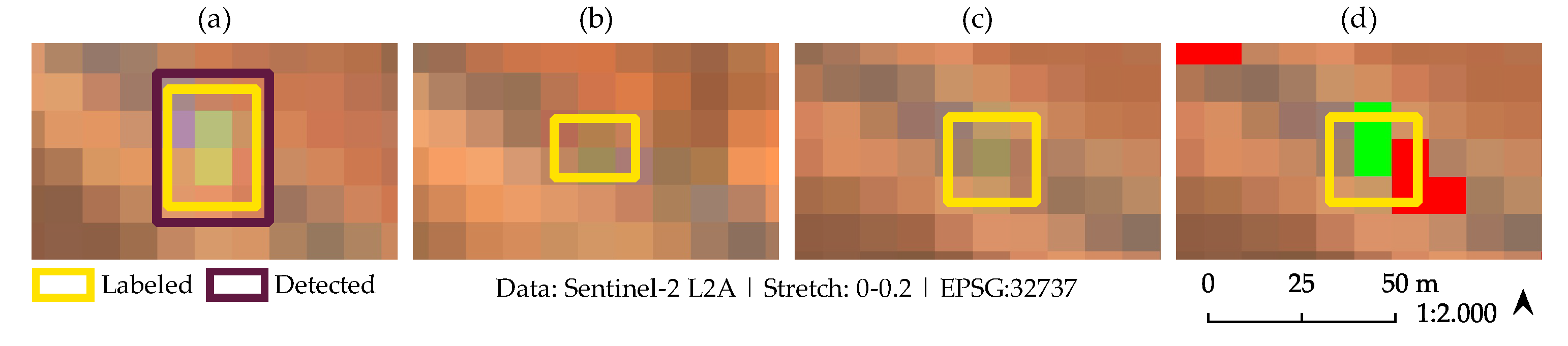
2.6.3. Detection Box Validation

Common practice in object detection evaluation is the comparison of predicted geometries with validation boxes [45,135]. The Sentinel-2 data were cropped to the extent of the labelled boxes (Section 2.4). Within this area, TP, FN, FP were calculated. A positive result was defined by the intersection over union $iou$. For each prediction box intersecting with a validation box, and vice versa, $iou$ was calculated as the ratio of the intersection area of the two boxes and the area of their union [135]. Only intersections with $iou$ > 0.25 were counted as positive. Commonly used is a threshold of 0.5 [45], however the target object in this work consists of very few pixels. The $iou$ can thus rapidly decrease yet when a box is one pixel smaller or larger. Based on TP, FN, FP, recall and precision were calculated and thereupon the F${}_1$ score. Trade-off between TP and FP was analyzed using the precision-recall-curve (PR) [126,127,130]. A range of detection score thresholds between 0 and 2 (maximum reachable score) was used for the PR curve.

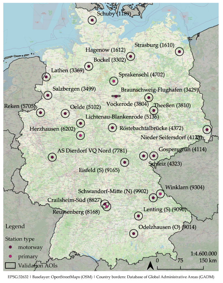
2.6.4. Traffic Count Station Validation

Traffic count data were obtained from 26 traffic count stations of the German Federal Highway Research Institute (BAST) [19] on motorways (A) and primary roads (B). Station counts deliver hourly traffic volumes [19]. At the primary level, the stations count motor vehicles (“KFZ”), summarizing car-like and truck-like vehicles of the second level. The truck-like class is further distinguished at the third level into cars with trailers, buses, trucks heavier 3.5 t without and with trailers. Trucks of this level are split into articulated trucks and trucks with trailer [136]. For validation, the vehicle class “Lastzug” (“Lzg”) was used. As of 2020 the most recent provided data covered 2018 [19]. Validation areas of interest (AOIs) are circular (Figure A1) except for the Braunschweig-Flughafen station where a rectangular buffer AOI was used to only cover the target highway. In these areas, the detection method was executed on all cloud-free Sentinel-2 L2A subsets in 2018. This sums up to 390 acquisitions (

Table A2. BAST traffic count stations and number of used Sentinel-2 acquisitions for the validation run.

	Station Name	Road Type	Used Acquisitions
1	AS Dierdof VQ Nord (7781)	A	14
2	Bockel (3302)	A	16
3	Braunschweig-Flughafen (3429)	A	24
4	Crailsheim-Süd (8827)	B	14
5	Eisfeld (S) (9165)	A	18
6	Gospersgrün (4114)	A	13
7	Hagenow (1612)	A	14
8	Herzhausen (6202)	B	9
9	Lathen (3369)	A	7
10	Lenting (S) (9090)	A	18
11	Lichtenau-Blankenrode (5136)	A	23
12	Nieder Seifersdorf (4123)	A	20
13	Oelde (5102)	A	16
14	Odelzhausen (O) (9014)	A	14
15	Reken (5705)	A	7
16	Reussenberg (8168)	A	14
17	Röstebachtalbrücke (4372)	A	8
18	Salzbergen (3499)	A	10
19	Schleiz (4323)	A	12
20	Schuby (1189)	A	17
21	Schwandorf-Mitte (N) (9902)	A	14
22	Sprakensehl (4702)	B	28
23	Strasburg (1610)	A	17
24	Theeßen (3810)	A	10
25	Vockerode (3804)	A	19
26	Winklarn (9304)	B	14
Sum			390

). 64% of these acquisitions originate from spring and summer months (April-September), 36% were acquired in autumn and winter months. The validation data were not balanced by season.

For comparing ground and remote sensing observations, Kaack et al. [43] generated a spatial mask derived from the average vehicle speed and a time interval. That is, only detected vehicles within this spatio-temporal buffer around a station were counted. The hourly station counts were scaled down to a 10 min interval within the hour of fully cloud-free Sentinel-2 acquisitions. Equivalent to the Sentinel-2 acquisition time, data of the 10 am truck count were used. A circular buffer with distance d around the station was calculated as in [43], based on an assumed 80 km/h average speed v, which is the German speed limit for trucks [137], and a 10 min time interval t:

$$d=v\times \frac{t}{60}.$$

(12)

Detections off the respective count station road type were masked out. The station data provide vehicle counts per hour ($nh$), hence the number of vehicles passing by t within 10 min in the Sentinel-2 acquisition hour was calculated as n:

$$n=nh\times \frac{t}{60},$$

(13)

assuming a stable traffic flow. This number contains only vehicles that passed by the station, whereas the Sentinel-2 detections cover the whole road. Thus, for each detection within the buffer, a vector between the station and the detection centroid coordinates was calculated. Using the same method for calculating the vehicle heading as in Section 2.5.8, the orientation of the detected vehicle in relation to the station was obtained. Postulating smooth roads, the angle between a vector pointing from the station to the detection and the heading vector of the detection should be smaller than 90° if the detection has yet passed the station. If fulfilled, the detection should not have been counted by the count station within t, and was thus excluded.

3. Results

3.1. Classifier Validation

The RF classifier has an overall accuracy of 84% (

Table 2. RF performance metrics.

	Precision	Recall	${\mathit{F}}_1$ Score	Support	Overall Accuracy
blue	0.91	0.87	0.89	350
green	0.9	0.86	0.88	350
red	0.87	0.79	0.83	350
background	0.73	0.86	0.79	350
Average	0.85	0.84	0.85
					0.84

) and a mean $F_1$ score of 0.85, with the lowest $F_1$ score observed for the background class (0.79). The confusion matrix (Figure A2) shows, red samples were most prone to being wrongly classified as background.

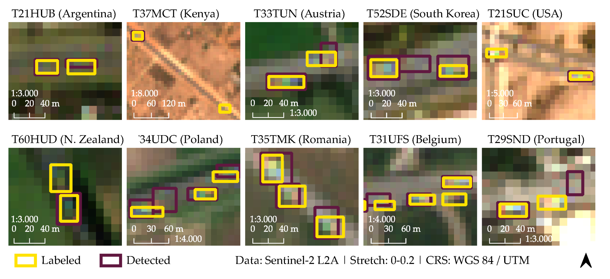
3.2. Detection Box Validation

The detection score (Section 2.5.7) was used to investigate a detection certainty threshold balancing precision and recall, expressed by the $F_1$ score (Section 2.6.1). A detection score of 1 on the x-axis (Figure 8) means that only detection boxes with a detection score > 1 were considered. The mean best detection score was 1.2 with a mean $F_1$ score of 0.74 (Figure 8). The highest $F_1$ score was yielded in Poland (0.88), the lowest in Kenya (0.36). Nine of ten AOIs yielded higher precision than recall, also apparent in the precision-recall (PR) curves (Figure 9).

Exemplary subsets of box validation AOIs provide a visual impression of the detection behavior compared to the validation boxes (Figure 10).

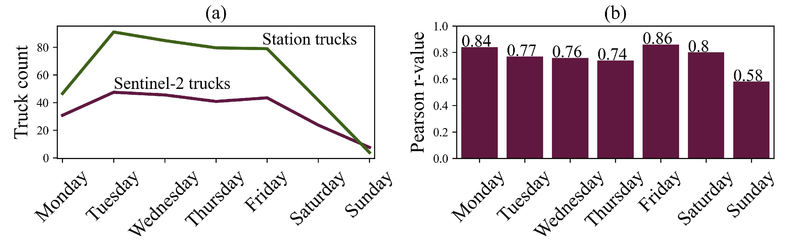
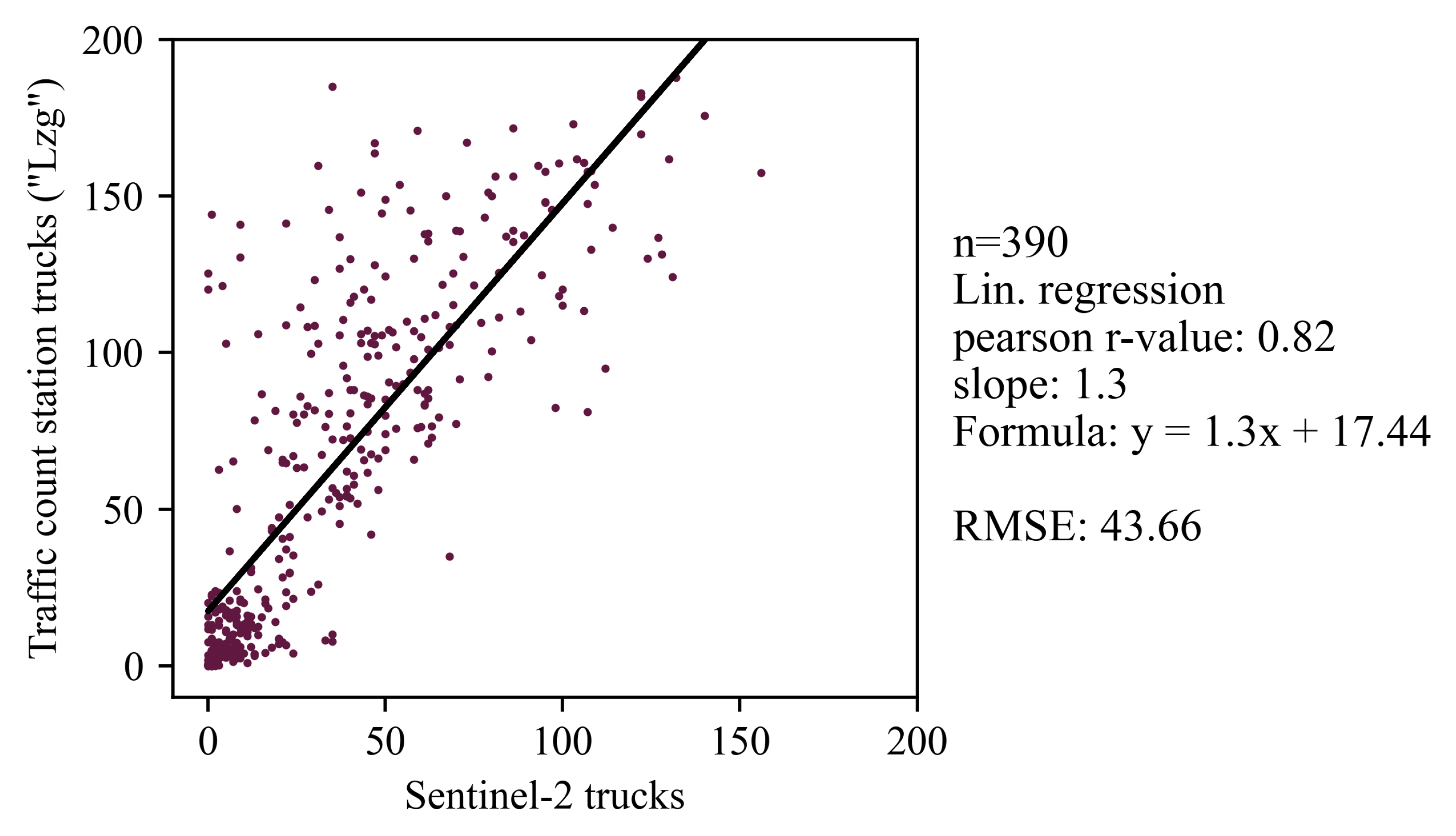
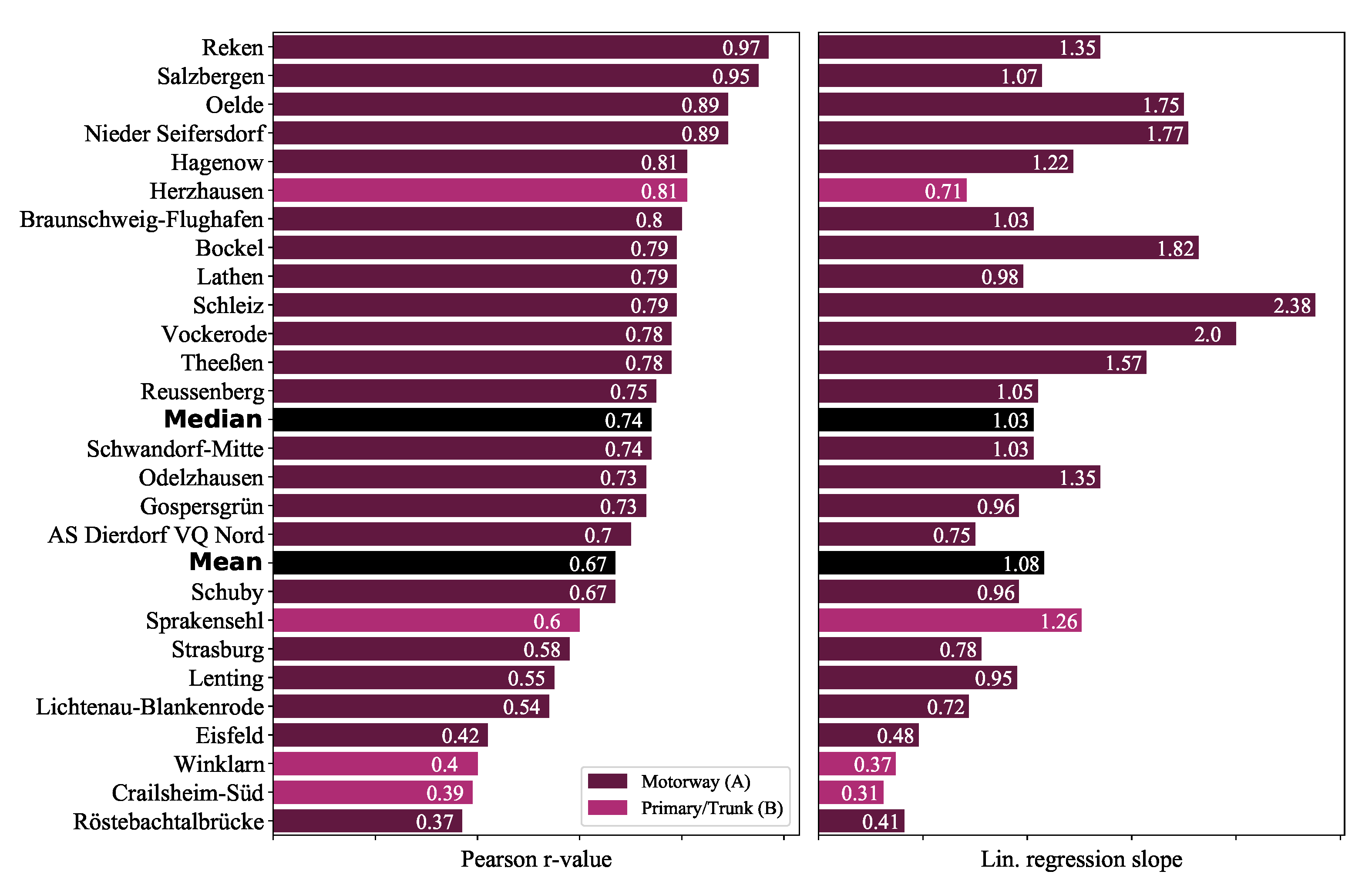
3.3. Traffic Count Station Validation

The Pearson r-value r of all compared Sentinel-2 and traffic count station truck figures is 0.82 with a linear regression slope of 1.3 and an intercept of 17.44 (Figure 11). Linear regression implies lower Sentinel-2 counts than station measurements. The RMSE between the station and Sentinel-2 figures is 43.7.

The standard deviation of the station counts and the Sentinel-2 counts is 54.98 and 34.45, respectively (

Table 3. Statistical summary of station and Sentinel-2 counts.

	Mean Count	Standard Deviation	Max. Count	Min. Count
Stations	63.18	54.98	206	0
Sentinel-2	35.14	34.45	170	0

). The mean truck number at the station (63.18) is higher than Sentinel-2 counts (35.14). On 81% of the processed acquisitions the Sentinel-2 method detected less trucks than traffic count stations (Table 3). In the 75th percentile, the station counted more trucks than the Sentinel-2 method for 98.98% of all values. In the 25th percentile, 52% of the counts were lower at the station than based on Sentinel-2.

Mean truck counts by weekday results in an r of 0.99 (Figure 12). Both methods have their average peak on Tuesday, and the lowest values on Sunday. Nearly all weekday mean values derived from Sentinel-2 are lower than the station values except Sunday (Figure 12).

Mean r values between traffic count station and Sentinel-2 truck counts based on the station-wise r is 0.67, the median 0.74 (Figure 13), with a maximum of 0.97 and a minimum of 0.37. Overall, r is above average at 65% of the traffic count stations. At 72% of the motorway stations (“Autobahn”), r is above average, while being below at 75% of the primary/trunk stations (“Bundesstraße”). Linear regression slopes widely imply a tendency to overestimate absolute counts where correlations are low, whereas high correlations are more often associated with high slopes suggesting underestimation (Figure 13).

Shown examples (Figure 14) are the station with the highest r value, two stations close to the 75th percentile of the r values of all stations, three stations close to the median, two stations close to the 25th percentile, and the station with the lowest r value. In addition, results from three stations on primary roads or trunks are shown. Corresponding detection maps include approximated speed, heading and detection scores (Figure 15). As observed in the whole dataset, the Sentinel-2 method usually detects fewer trucks than the traffic count stations. Predominant underestimation of the Sentinel-2-based truck counts compared to station measurements is confirmed by the regression results. In general, there are noticeable variations of counted trucks supported both by the stations and the Sentinel-2 counts. For instance, at Braunschweig-Flughafen, the station counts reach 206 on 10 April (Sentinel-2: 170), whereas they are down to 4 (Sentinel-2: 13) on 20 May. At Lenting, 22 April and 29 April (both Sunday) were captured with low counts. 2 April (Easter Monday) has similar low counts. Many examples can be found where such an agreement is not given. Furthermore, a cluster of unusual strong deviations between both count methods is observed on several dates in February, with the station count being on at least average level and the Sentinel-2 counts close to 0. This is seen e.g., on 21 and 23 February at Schwandorf-Mitte, 28 February at Odelzhausen, and 8 and 28 February at Strasburg. At Schwandorf-Mitte on 21 February, the station counted 72 trucks more than the Sentinel-2 method.

Apart from collective spatio-temporal truck abundance, each truck carries speed and heading properties. Example maps of detections in six box validation AOIs provide an impression of these properties and the detection scores with underlaid VIS reflectances (Figure 15).

3.3.1. Relationship between Sentinel-2 Truck Counts and Station Truck Types

The traffic count station truck classes differ in their agreement with the Sentinel-2 truck counts (Figure 16). In the validation, “Lzg” (“articulated truck”) was used, containing “Sat”, a truck always pulling a trailer, and “LmA”, a truck-like vehicle (heavier than 3.5 t) with a trailer. “Lkw” summarizes all truck-like vehicles, including buses and cars with a trailer and trucks without a trailer [136,138]. While the variation agreement is similar for all classes given an r value of 0.81 to 0.82, “Sat” has a slope close to 1 (1.06) and the lowest intercept of all classes (14.51).

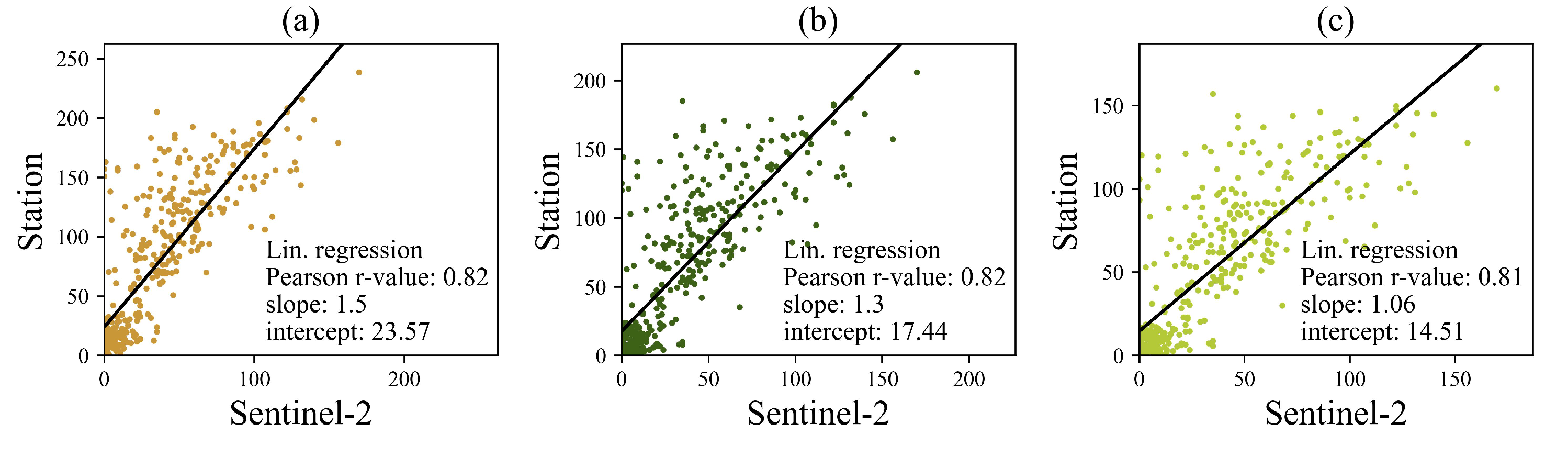
3.3.2. Relationship between Sentinel-2 Truck Counts and Station Car Counts

The r value of Sentinel-2 truck counts and the car station counts is 0.63. On average, the Sentinel-2 truck counts are 8.5% of the station car counts. Station car-like vehicle counts have a different magnitude than the station and the Sentinel-2 truck counts (Figure 17). Yet, some variations are shared (r in Figure 17 between 0.48 and 0.65).

4. Discussion

The presented moving truck detection based on multispectral Sentinel-2 data agrees well with globally labelled target objects in most tested countries. Detected trucks correlate spatio-temporally with truck figures provided by traffic count stations in Germany with a tendency to be underestimated by the Sentinel-2-based method. The method performs best where trucks travel fast and are distinguishable from the background. Limitations and weaknesses are discussed in the following.

4.1. Detection Performance and Validation

The moving truck detection method partly relies on an RF classifier with an overall accuracy of 84%. Confusions mainly occurred between the three target anomaly classes and the background class. Confusions have occurred particularly in the box validation area in Kenya, which reached the lowest $F_1$ score. A comparably low recall drives this low score, while the precision is high. The Kenyan box validation area is an example where some of the labelled targets (Figure 18) are difficult to distinguish from the background. The classification (a in Figure 18) exemplifies that the assumed blue anomaly pixel was not predicted here. Similar challenges regarding the manually labelled validation boxes were observed in the US-American validation area. These examples imply that differentiation from the background is not always successful and depends on local road conditions and types. Particularly bright road surfaces seem to decrease detection performance. Balancing the training and validation dataset by road type and weather conditions was not done here, and should be examined in the future.

Apart from these problematic areas, however, the agreement with validation boxes is satisfactory. It can also be stated that the detection performance seems not biased towards European countries, although 50% of the training and validation objects were collected in European countries. Four of the six highest $F_1$ scores were obtained in European validation areas. The box validation results suggest global applicability, though local performance differences should be kept in mind.

Only ground truth data inform about the relationship to real-world vehicles and vehicle types. Validation with such data has yet been limited to the traffic count station network in Germany. There is a strong relationship between counted trucks at traffic count stations in Germany and trucks detected by the Sentinel-2 method, given an r of 0.82. Overall, a tendency to lower Sentinel-2-based detections than station counts was observed. Moreover, the Sentinel-2 method tends to particularly underestimate the counts in peak traffic situations. It was shown that the Sentinel-2 method nearly never overestimated figures in these peak situations, whereas in nearly half of the low traffic situations the Sentinel-2 counts exceeded the station counts. Two reasons are likely: (1) we must assume that there are several false detections that are independent of the true truck traffic. When counts are low the false detection noise will be a higher percentage of the final counts. (2) congested but still moving traffic situations could lead to an underestimation due to low speed. Validating these conclusions would require comparing spatio-temporal traffic congestion data with detections.

On average, weekday variations were similarly captured by the traffic count station data in Germany and the Sentinel-2-based counts. Sunday, Easter, and Christmas minimums were frequently detected in agreement with the station data. These are coarse patterns, finer variations among working days occurred only occasionally. The validation at traffic count stations shows that agreements are better on highways than on primary roads. It is crucial to consider that, in low count settings, already slight differences strongly impact the agreement. Still, the counts are within the correct magnitude. Systematic truck count underestimations by the Sentinel-2 method were observed at several stations in February 2018. A closer look shows that in particular acquisitions in Strasburg, Reussenberg, and Röstebachtalbrücke were affected by snow cover (Figure 19), caused by a cold spell in February 2018 [139]. The VIS reflectance values besides the roads, partly also covering the roads, are widely close to saturation. Also visually, nearly no assumed target objects could be identified in the acquisitions. Two reasons are likely: (1) caused by the problematic weather conditions, trucks might have been too slow for being visible and detectable, (2) the detection method fails due to many saturated pixels. Once many pixels are highly reflective, the subtraction of the overall band mean values from the reflectance values is likely to result in negative values. This could be tackled by calculating the band mean values only based on reflectance values below a threshold. Here, it is important to generally note that the band mean values differ depending on the AOI. The snowy observations combined with the partly low detection performance in the box validation areas in the USA and Kenya confirm that temporary or constant conditions of the surrounding may affect the truck detection adversely. Hence, local applicability should be at least subject to plausibility checks.

The validation at traffic count stations in Germany implies good agreements with truck counts of the station class “Lzg”, which summarizes large trucks and buses within the main class “Lkw” (trucks). “Lzg” contains “Sat” (long articulated trucks). Consequently, the best agreement was found between the Sentinel-2 counts and the “Sat” class. This implies that the Sentinel-2 moving truck detection method is most suited for detecting large trucks. Station counts of the “KFZ” class (car-like vehicles) are on average the 12-fold of the Sentinel-2 detections. Yet, there is a correlation (r: 0.63) between the number of counted cars and the Sentinel-2 trucks. Although the relationship may differ in other areas of the world, this result suggests the potential of extrapolating general road traffic density based on the Sentinel-2 moving truck detection, at least where other data sources are sparse. The detection performance evaluation using manually labelled target boxes, and the station-based validation combined, suggest applicability beyond Germany. Further validation approaches in other regions would be favorable. Other reference data sources could be employed, for instance, traffic webcam data [140].

Furthermore, CNNs could be tested for detecting moving trucks in Sentinel-2 data. Here, the emphasis should be on the small size of the objects, which usually consist of three to eight pixels. This was the main reason why CNNs were not used in this study. A CNN infrastructure will have to take the small object size into account [100,101,102].

The presented method is closely tied to Sentinel-2 data by exploiting the specific MSI sensor layout [56] and resulting reflectance effects. Transferring the specific procedure to other remote sensing data sources such as unmanned aerial vehicles (UAV) [141] or satellite sensors is thus not straight forward. However, the concept of motion detection and velocity approximation through a sequence of images has been used for many years [18,58,59,60,78].

4.2. Applications

Bearing in mind data-related limitations such as cloud cover and revisit time, the Sentinel-2 truck detection method may be well suited to fill gaps, especially in areas where data on road cargo traffic counts are sparse. Information on truck abundance can serve as a proxy for economic activity: In Germany, an index based on truck toll provides near real-time information on truck traffic and thereby also information on economic performance [12]. Li et al. revealed that among different vehicle types in China truck traffic is the second most important predictor for the gross domestic product [13]. Boarnet et al. [11] found strong positive correlations between road cargo density and employment in urban sub-centers of Los Angeles. Economy, cargo traffic and its environmental impact are closely related; we have seen the impact of systematic disruptions of economies e.g., on air pollution during the COVID-19 pandemic [14,15,16]. Sentinel-2-based moving truck detection is applicable in areas where little or no other data sources exist, including regions that are difficult to access, e.g., in sub-Saharan Africa. For instance, we could imagine to regularly apply the method in areas where illegal mining or deforestation is undertaken. By detecting truck count anomalies, the method could even be an addition e.g., to conservation early warning systems [142].

5. Conclusions

For the first time, a moving truck detection method based on Sentinel-2 MSI data was presented. We have demonstrated that, due to temporal sensing offsets of the Sentinel-2 spectral bands, moving vehicles of truck size are visible and detectable at 10 m spatial resolution. The developed moving truck detection method performs well in most globally tested countries. It agrees with spatio-temporal truck figures from traffic count stations in Germany, however, the method tends to underestimate absolute truck counts. Detecting large and fast trucks works best. The temporal coverage of the Sentinel-2 data and the accuracy of absolute counts are inferior to continuous monitoring by traffic count stations. Compared to truck detection based on very high resolution aerial and satellite remote sensing data, the advantage of the Sentinel-2-based moving truck detection is its systematic and free global coverage. Due to varying road surfaces, truck speed, and size, further checks and optimally local validations will be required. Provided careful considerations, the Sentinel-2 moving truck detection method may be a valuable addition to research and applications by providing a proxy for cargo traffic, emissions, and economic activities, particularly in areas with sparse other data sources.

References

1. Novotny, E.V.; Bechle, M.J.; Millet, D.B.; Marshall, J.D. National satellite-based land-use regression: NO2 in the United States. Environ. Sci. Technol. 2011, 45, 4407–4414. [Google Scholar] [CrossRef] [PubMed]
2. Beevers, S.D.; Westmoreland, E.; de Jong, M.C.; Williams, M.L.; Carslaw, D.C. Trends in NOx and NO2 emissions from road traffic in Great Britain. Atmos. Environ. 2012, 54, 107–116. [Google Scholar] [CrossRef]
3. Saucy, A.; Röösli, M.; Künzli, N.; Tsai, M.Y.; Sieber, C.; Olaniyan, T.; Baatjies, R.; Jeebhay, M.; Davey, M.; Flückiger, B.; et al. Land Use Regression Modelling of Outdoor NO2 and PM2.5 Concentrations in Three Low Income Areas in the Western Cape Province, South Africa. Int. J. Environ. Res. Public Health 2018, 15, 1452. [Google Scholar] [CrossRef] [PubMed] [Green Version]
4. European Environment Agency. Air Quality in Europe—2019 Report; European Environment Agency: Copenhagen, Denmark, 2019.
5. Harrison, R.M.; Vu, T.V.; Jafar, H.; Shi, Z. More mileage in reducing urban air pollution from road traffic. Environ. Int. 2021, 149, 106329. [Google Scholar] [CrossRef]
6. European Union Eurostat. Freight Transport Statistics; European Union Eurostat: Luxembourg, 2020.
7. Organization for Economic Cooperation. OECD Data—Freight Transport; Organization for Economic Cooperation: Paris, France, 2021. [Google Scholar]
8. Bureau of Transportation Statistics. Freight Shipments by Mode; Bureau of Transportation Statistics: Washington, DC, USA, 2020.
9. Huo, H.; Yao, Z.; Zhang, Y.; Shen, X.; Zhang, Q.; He, K. On-board measurements of emissions from diesel trucks in five cities in China. Atmos. Environ. 2012, 54, 159–167. [Google Scholar] [CrossRef]
10. Liimatainen, H.; van Vliet, O.; Aplyn, D. The potential of electric trucks—An international commodity-level analysis. Appl. Energy 2019, 236, 804–814. [Google Scholar] [CrossRef]
11. Boarnet, M.G.; Hong, A.; Santiago-Bartolomei, R. Urban spatial structure, employment subcenters, and freight travel. J. Transport Geogr. 2017, 60, 267–276. [Google Scholar] [CrossRef]
12. Deutsches Statistisches Bundesamt (DESTATIS). Truck Toll Mileage Index; Deutsches Statistisches Bundesamt: Wiesbaden, Germany, 2020.
13. Li, B.; Gao, S.; Liang, Y.; Kang, Y.; Prestby, T.; Gao, Y.; Xiao, R. Estimation of Regional Economic Development Indicator from Transportation Network Analytics. Sci. Rep. 2020, 10, 2647. [Google Scholar] [CrossRef]
14. Berman, J.D.; Ebisu, K. Changes in U.S. air pollution during the COVID-19 pandemic. Sci. Total Environ. 2020, 739, 139864. [Google Scholar] [CrossRef]
15. Venter, Z.S.; Aunan, K.; Chowdhury, S.; Lelieveld, J. COVID-19 lockdowns cause global air pollution declines. Proc. Natl. Acad. Sci. USA 2020, 117, 18984–18990. [Google Scholar] [CrossRef]
16. Chan, K.L.; Khorsandi, E.; Liu, S.; Baier, F.; Valks, P. Estimation of Surface NO2 Concentrations over Germany from TROPOMI Satellite Observations Using a Machine Learning Method. Remote Sens. 2021, 13, 969. [Google Scholar] [CrossRef]
17. Bernas, M.; Płaczek, B.; Korski, W.; Loska, P.; Smyła, J.; Szymała, P. A Survey and Comparison of Low-Cost Sensing Technologies for Road Traffic Monitoring. Sensors 2018, 18, 3243. [Google Scholar] [CrossRef] [PubMed] [Green Version]
18. Rosenbaum, D.; Kurz, F.; Thomas, U.; Suri, S.; Reinartz, P. Towards automatic near real-time traffic monitoring with an airborne wide angle camera system. Eur. Transp. Res. Rev. 2009, 1, 11–21. [Google Scholar] [CrossRef] [Green Version]
19. Bundesanstalt für Straßenwesen. Automatische Zählstellen auf Autobahnen und Bundesstraßen; Bundesanstalt für Straßenwesen: Bergisch Gladbach, Germany, 2021.
20. Federal Highway Administration. U.S. Traffic Monitoring Location Data; Federal Highway Administration: Washington, DC, USA, 2020.
21. Autobahnen- und Schnellstraßen-Finanzierungs-Aktiengesellschaft. Verkehrsentwicklung; Autobahnen- und Schnellstraßen-Finanzierungs-Aktiengesellschaft: Vienna, Austria, 2021. [Google Scholar]
22. Bottero, M.; Dalla Chiara, B.; Deflorio, F. Wireless sensor networks for traffic monitoring in a logistic centre. Transp. Res. Part C Emerg. Technol. 2013, 26, 99–124. [Google Scholar] [CrossRef]
23. Gerhardinger, A.; Ehrlich, D.; Pesaresi, M. Vehicles detection from very high resolution satellite imagery. Int. Arch. Photogramm. Remote Sens. 2005, 36, W24. [Google Scholar]
24. Datondji, S.R.E.; Dupuis, Y.; Subirats, P.; Vasseur, P. A Survey of Vision-Based Traffic Monitoring of Road Intersections. IEEE Trans. Intell. Transport. Syst. 2016, 17, 2681–2698. [Google Scholar] [CrossRef]
25. Janecek, A.; Valerio, D.; Hummel, K.A.; Ricciato, F.; Hlavacs, H. The Cellular Network as a Sensor: From Mobile Phone Data to Real-Time Road Traffic Monitoring. IEEE Trans. Intell. Transport. Syst. 2015, 16, 2551–2572. [Google Scholar] [CrossRef]
26. Wang, D.; Al-Rubaie, A.; Davies, J.; Clarke, S.S. Real time road traffic monitoring alert based on incremental learning from tweets. In Proceedings of the 2014 IEEE Symposium on Evolving and Autonomous Learning Systems (EALS), Orlando, FL, USA, 9–12 December 2014; pp. 50–57. [Google Scholar] [CrossRef]
27. Nellore, K.; Hancke, G. A Survey on Urban Traffic Management System Using Wireless Sensor Networks. Sensors 2016, 16, 157. [Google Scholar] [CrossRef] [Green Version]
28. Chen, Y.; Qin, R.; Zhang, G.; Albanwan, H. Spatial Temporal Analysis of Traffic Patterns during the COVID-19 Epidemic by Vehicle Detection Using Planet Remote-Sensing Satellite Images. Remote Sens. 2021, 13, 208. [Google Scholar] [CrossRef]
29. Bouguettaya, A.; Zarzour, H.; Kechida, A.; Taberkit, A.M. Vehicle Detection From UAV Imagery with Deep Learning: A Review. IEEE Trans. Neural Netw. Learn. Syst. 2021, 1–21. [Google Scholar] [CrossRef]
30. Charouh, Z.; Ezzouhri, A.; Ghogho, M.; Guennoun, Z. A Resource-Efficient CNN-Based Method for Moving Vehicle Detection. Sensors 2022, 22, 1193. [Google Scholar] [CrossRef] [PubMed]
31. Ghasemi Darehnaei, Z.; Rastegar Fatemi, S.M.J.; Mirhassani, S.M.; Fouladian, M. Ensemble Deep Learning Using Faster R-CNN and Genetic Algorithm for Vehicle Detection in UAV Images. IETE J. Res. 2021, 1–10. [Google Scholar] [CrossRef]
32. Maity, M.; Banerjee, S.; Sinha Chaudhuri, S. Faster R-CNN and YOLO based Vehicle detection: A Survey. In Proceedings of the 2021 5th International Conference on Computing Methodologies and Communication (ICCMC), Erode, India, 8–10 April 2021; pp. 1442–1447. [Google Scholar] [CrossRef]
33. Luo, X.; Tian, X.; Zhang, H.; Hou, W.; Leng, G.; Xu, W.; Jia, H.; He, X.; Wang, M.; Zhang, J. Fast Automatic Vehicle Detection in UAV Images Using Convolutional Neural Networks. Remote Sens. 2020, 12, 1994. [Google Scholar] [CrossRef]
34. Koga, Y.; Miyazaki, H.; Shibasaki, R. A Method for Vehicle Detection in High-Resolution Satellite Images that Uses a Region-Based Object Detector and Unsupervised Domain Adaptation. Remote Sens. 2020, 12, 575. [Google Scholar] [CrossRef] [Green Version]
35. Zhang, Z.; Liu, Y.; Liu, T.; Lin, Z.; Wang, S. DAGN: A Real-Time UAV Remote Sensing Image Vehicle Detection Framework. IEEE Geosci. Remote Sens. Lett. 2020, 17, 1884–1888. [Google Scholar] [CrossRef]
36. Tan, Q.; Ling, J.; Hu, J.; Qin, X.; Hu, J. Vehicle Detection in High Resolution Satellite Remote Sensing Images Based on Deep Learning. IEEE Access 2020, 8, 153394–153402. [Google Scholar] [CrossRef]
37. Yao, H.; Qin, R.; Chen, X. Unmanned Aerial Vehicle for Remote Sensing Applications—A Review. Remote Sens. 2019, 11, 1443. [Google Scholar] [CrossRef] [Green Version]
38. Ji, H.; Gao, Z.; Mei, T.; Li, Y. Improved Faster R-CNN with Multiscale Feature Fusion and Homography Augmentation for Vehicle Detection in Remote Sensing Images. IEEE Geosci. Remote Sens. Lett. 2019, 16, 1761–1765. [Google Scholar] [CrossRef]
39. Wang, L.; Liao, J.; Xu, C. Vehicle Detection Based on Drone Images with the Improved Faster R-CNN. In Proceedings of the 2019 11th International Conference on Machine Learning and Computing—ICMLC ’19, Zhuhai, China, 22–24 February 2019; pp. 466–471. [Google Scholar] [CrossRef]
40. Yu, Y.; Gu, T.; Guan, H.; Li, D.; Jin, S. Vehicle Detection From High-Resolution Remote Sensing Imagery Using Convolutional Capsule Networks. IEEE Geosci. Remote Sens. Lett. 2019, 16, 1894–1898. [Google Scholar] [CrossRef]
41. Tao, C.; Mi, L.; Li, Y.; Qi, J.; Xiao, Y.; Zhang, J. Scene Context-Driven Vehicle Detection in High-Resolution Aerial Images. IEEE Trans. Geosci. Remote Sens. 2019, 57, 7339–7351. [Google Scholar] [CrossRef]
42. Zheng, K.; Wei, M.; Sun, G.; Anas, B.; Li, Y. Using Vehicle Synthesis Generative Adversarial Networks to Improve Vehicle Detection in Remote Sensing Images. ISPRS Int. J. Geo-Inf. 2019, 8, 390. [Google Scholar] [CrossRef] [Green Version]
43. Kaack, L.H.; Chen, G.H.; Morgan, M.G. Truck traffic monitoring with satellite images. In Proceedings of the Conference on Computing & Sustainable Societies—COMPASS 19, Accra, Ghana, 3–5 July 2019; pp. 155–164. [Google Scholar] [CrossRef] [Green Version]
44. Yang, M.Y.; Liao, W.; Li, X.; Cao, Y.; Rosenhahn, B. Vehicle Detection in Aerial Images. Photogramm. Eng. Remote Sens. 2019, 85, 297–304. [Google Scholar] [CrossRef] [Green Version]
45. Audebert, N.; Le Saux, B.; Lefèvre, S. Segment-before-Detect: Vehicle Detection and Classification through Semantic Segmentation of Aerial Images. Remote Sens. 2017, 9, 368. [Google Scholar] [CrossRef] [Green Version]
46. Deng, Z.; Sun, H.; Zhou, S.; Zhao, J.; Zou, H. Toward Fast and Accurate Vehicle Detection in Aerial Images Using Coupled Region-Based Convolutional Neural Networks. IEEE J. Sel. Top. Appl. Earth Obs. Remote Sens. 2017, 10, 3652–3664. [Google Scholar] [CrossRef]
47. Sakai, K.; Seo, T.; Fuse, T. Traffic density estimation method from small satellite imagery: Towards frequent remote sensing of car traffic. In Proceedings of the 2019 IEEE Intelligent Transportation Systems Conference (ITSC), Auckland, New Zealand, 27–30 October 2019; pp. 1776–1781. [Google Scholar] [CrossRef]
48. Koga, Y.; Miyazaki, H.; Shibasaki, R. A CNN-Based Method of Vehicle Detection from Aerial Images Using Hard Example Mining. Remote Sens. 2018, 10, 124. [Google Scholar] [CrossRef] [Green Version]
49. Tayara, H.; Gil Soo, K.; Chong, K.T. Vehicle Detection and Counting in High-Resolution Aerial Images Using Convolutional Regression Neural Network. IEEE Access 2018, 6, 2220–2230. [Google Scholar] [CrossRef]
50. Yang, T.; Wang, X.; Yao, B.; Li, J.; Zhang, Y.; He, Z.; Duan, W. Small Moving Vehicle Detection in a Satellite Video of an Urban Area. Sensors 2016, 16, 1528. [Google Scholar] [CrossRef] [Green Version]
51. Heiselberg, P.; Heiselberg, H. Aircraft Detection above Clouds by Sentinel-2 MSI Parallax. Remote Sens. 2021, 13, 3016. [Google Scholar] [CrossRef]
52. Heiselberg, H. Aircraft and Ship Velocity Determination in Sentinel-2 Multispectral Images. Sensors 2019, 19, 2873. [Google Scholar] [CrossRef] [Green Version]
53. Frantz, D.; Haß, E.; Uhl, A.; Stoffels, J.; Hill, J. Improvement of the Fmask algorithm for Sentinel-2 images: Separating clouds from bright surfaces based on parallax effects. Remote Sens. Environ. 2018, 215, 471–481. [Google Scholar] [CrossRef]
54. Gascon, F.; Bouzinac, C.; Thépaut, O.; Jung, M.; Francesconi, B.; Louis, J.; Lonjou, V.; Lafrance, B.; Massera, S.; Gaudel-Vacaresse, A.; et al. Copernicus Sentinel-2A Calibration and Products Validation Status. Remote Sens. 2017, 9, 584. [Google Scholar] [CrossRef] [Green Version]
55. Skakun, S.; Vermote, E.; Roger, J.C.; Justice, C. Multispectral Misregistration of Sentinel-2A Images: Analysis and Implications for Potential Applications. IEEE Geosci. Remote Sens. Lett. 2017, 14, 2408–2412. [Google Scholar] [CrossRef] [PubMed]
56. Gatti, A.; Bertolini, A. Sentinel-2 Products Specification Document; European Space Agency: Paris, France, 2015. [Google Scholar]
57. Börner, A.; Ernst, I.; Ruhé, M.; Zujew, S. Airborne Camera Experiments for Traffic Monitoring. In Proceedings of the ISPRS—10th Congress International Society for Photogrammetry and Remote Sensing, Istanbul, Turkey, 12–23 July 2004. [Google Scholar]
58. Reinartz, P.; Lachaise, M.; Schmeer, E.; Krauss, T.; Runge, H. Traffic monitoring with serial images from airborne cameras. ISPRS J. Photogramm. Remote Sens. 2006, 61, 149–158. [Google Scholar] [CrossRef]
59. Palubinskas, G.; Kurz, F.; Reinartz, P. Detection of Traffic Congestion in Optical Remote Sensing Imagery. In Proceedings of the IGARSS 2008, 2008 IEEE International Geoscience and Remote Sensing Symposium, Boston, MA, USA, 7–11 July 2008; pp. II-426–II-429. [Google Scholar] [CrossRef] [Green Version]
60. Leitloff, J.; Rosenbaum, D.; Kurz, F.; Meynberg, O.; Reinartz, P. An Operational System for Estimating Road Traffic Information from Aerial Images. Remote Sens. 2014, 6, 11315–11341. [Google Scholar] [CrossRef] [Green Version]
61. Yao, W.; Zhang, M.; Hinz, S.; Stilla, U. Airborne traffic monitoring in large areas using LiDAR data—Theory and experiments. Int. J. Remote Sens. 2012, 33, 3930–3945. [Google Scholar] [CrossRef]
62. Suchandt, S.; Runge, H.; Breit, H.; Steinbrecher, U.; Kotenkov, A.; Balss, U. Automatic Extraction of Traffic Flows Using TerraSAR-X Along-Track Interferometry. IEEE Trans. Geosci. Remote Sens. 2010, 48, 807–819. [Google Scholar] [CrossRef]
63. Meyer, F.; Hinz, S.; Laika, A.; Weihing, D.; Bamler, R. Performance analysis of the TerraSAR-X Traffic monitoring concept. ISPRS J. Photogramm. Remote Sens. 2006, 61, 225–242. [Google Scholar] [CrossRef]
64. Hinz, S.; Leitloff, J.; Stilla, U. Context-supported vehicle detection in optical satellite images of urban areas. In Proceedings of the 2005 IEEE International Geoscience and Remote Sensing Symposium, Seoul, Korea, 25–29 July 2005; Volume 4, pp. 2937–2941. [Google Scholar] [CrossRef]
65. Larsen, S.Ø.; Koren, H.; Solberg, R. Traffic Monitoring using Very High Resolution Satellite Imagery. Photogramm. Eng. Remote Sens. 2009, 75, 859–869. [Google Scholar] [CrossRef] [Green Version]
66. Blaschke, T. Object based image analysis for remote sensing. ISPRS J. Photogramm. Remote Sens. 2010, 65, 2–16. [Google Scholar] [CrossRef] [Green Version]
67. Gao, F.; Li, B.; Xu, Q.; Zhong, C. Moving Vehicle Information Extraction from Single-Pass WorldView-2 Imagery Based on ERGAS-SNS Analysis. Remote Sens. 2014, 6, 6500–6523. [Google Scholar] [CrossRef] [Green Version]
68. Bar, D.E.; Raboy, S. Moving Car Detection and Spectral Restoration in a Single Satellite WorldView-2 Imagery. IEEE J. Sel. Top. Appl. Earth Obs. Remote Sens. 2013, 6, 2077–2087. [Google Scholar] [CrossRef]
69. Pesaresi, M.; Gutjahr, K.H.; Pagot, E. Estimating the velocity and direction of moving targets using a single optical VHR satellite sensor image. Int. J. Remote Sens. 2008, 29, 1221–1228. [Google Scholar] [CrossRef]
70. Du, B.; Cai, S.; Wu, C. Object Tracking in Satellite Videos Based on a Multiframe Optical Flow Tracker. IEEE J. Sel. Top. Appl. Earth Obs. Remote Sens. 2019, 12, 3043–3055. [Google Scholar] [CrossRef] [Green Version]
71. Ahmadi, S.A.; Ghorbanian, A.; Mohammadzadeh, A. Moving vehicle detection, tracking and traffic parameter estimation from a satellite video: A perspective on a smarter city. Int. J. Remote Sens. 2019, 40, 8379–8394. [Google Scholar] [CrossRef]
72. Toth, C.; Jóźków, G. Remote sensing platforms and sensors: A survey. ISPRS J. Photogramm. Remote Sens. 2016, 115, 22–36. [Google Scholar] [CrossRef]
73. Kopsiaftis, G.; Karantzalos, K. Vehicle detection and traffic density monitoring from very high resolution satellite video data. In Proceedings of the 2015 IEEE International Geoscience and Remote Sensing Symposium (IGARSS), Milan, Italy, 26–31 July 2015; pp. 1881–1884. [Google Scholar] [CrossRef]
74. Chang, Y.; Wang, S.; Zhou, Y.; Wang, L.; Wang, F. A Novel Method of Evaluating Highway Traffic Prosperity Based on Nighttime Light Remote Sensing. Remote Sens. 2019, 12, 102. [Google Scholar] [CrossRef] [Green Version]
75. Tang, T.; Zhou, S.; Deng, Z.; Lei, L.; Zou, H. Arbitrary-Oriented Vehicle Detection in Aerial Imagery with Single Convolutional Neural Networks. Remote Sens. 2017, 9, 1170. [Google Scholar] [CrossRef] [Green Version]
76. Drusch, M.; Del Bello, U.; Carlier, S.; Colin, O.; Fernandez, V.; Gascon, F.; Hoersch, B.; Isola, C.; Laberinti, P.; Martimort, P.; et al. Sentinel-2: ESA’s Optical High-Resolution Mission for GMES Operational Services. Remote Sens. Environ. 2012, 120, 25–36. [Google Scholar] [CrossRef]
77. European Space Agency. Multi Spectral Instrument (MSI) Overview; European Space Agency: Paris, France, 2020. [Google Scholar]
78. Kääb, A.; Leprince, S. Motion detection using near-simultaneous satellite acquisitions. Remote Sens. Environ. 2014, 154, 164–179. [Google Scholar] [CrossRef] [Green Version]
79. Meng, L.; Kerekes, J.P. Object Tracking Using High Resolution Satellite Imagery. IEEE J. Sel. Top. Appl. Earth Obs. Remote Sens. 2012, 5, 146–152. [Google Scholar] [CrossRef] [Green Version]
80. Easson, G.; DeLozier, S.; Momm, H.G. Estimating Speed and Direction of Small Dynamic Targets through Optical Satellite Imaging. Remote Sens. 2010, 2, 1331–1347. [Google Scholar] [CrossRef] [Green Version]
81. Liu, Y.; Xu, B.; Zhi, W.; Hu, C.; Dong, Y.; Jin, S.; Lu, Y.; Chen, T.; Xu, W.; Liu, Y.; et al. Space eye on flying aircraft: From Sentinel-2 MSI parallax to hybrid computing. Remote Sens. Environ. 2020, 246, 111867. [Google Scholar] [CrossRef]
82. Council of the European Union. COUNCIL DIRECTIVE 96/53/EC; European Union: Brussels, Belgium, 1997. [Google Scholar]
83. National Heavy Vehicle Regulator. Common Heavy Freight Vehicle Configurations; National Heavy Vehicle Regulator: Newstead, Australia, 2017.
84. Strahler, A.H.; Woodcock, C.E.; Smith, J.A. On the nature of models in remote sensing. Remote Sens. Environ. 1986, 20, 121–139. [Google Scholar] [CrossRef]
85. European Space Agency. Euro Data Cube Custom Script Contest: The Winner Is…; European Space Agency: Paris, France, 2020. [Google Scholar]
86. Fisser, H. Truck Detection Using Sentinel-2 Data; University of Wuerzburg: Wuerzburg, Germany, 2020. [Google Scholar]
87. Verschae, R.; Ruiz-del Solar, J. Object Detection: Current and Future Directions. Front. Robot. AI 2015, 2, 29. [Google Scholar] [CrossRef] [Green Version]
88. Jain, A.K.; Ratha, N.K.; Lakshmanan, S. Object detection using gabor filters. Patt. Recognit. 1997, 30, 295–309. [Google Scholar] [CrossRef]
89. Trivedi, M.M.; Harlow, C.A.; Conners, R.W.; Goh, S. Object detection based on gray level cooccurrence. Comput. Vis. Graph. Image Process. 1984, 28, 199–219. [Google Scholar] [CrossRef]
90. Shaikh, S.H.; Saeed, K.; Chaki, N. Moving Object Detection Using Background Subtraction. In Moving Object Detection Using Background Subtraction; Series Title: SpringerBriefs in Computer Science; Springer International Publishing: Cham, Switzerland, 2014; pp. 15–23. [Google Scholar] [CrossRef]
91. Piccardi, M. Background subtraction techniques: A review. In Proceedings of the 2004 IEEE International Conference on Systems, Man and Cybernetics (IEEE Cat. No.04CH37583), The Hague, The Netherlands, 10–13 October 2004; pp. 3099–3104. [Google Scholar] [CrossRef] [Green Version]
92. Hoeser, T.; Kuenzer, C. Object Detection and Image Segmentation with Deep Learning on Earth Observation Data: A Review-Part I: Evolution and Recent Trends. Remote Sens. 2020, 12, 1667. [Google Scholar] [CrossRef]
93. Li, K.; Wan, G.; Cheng, G.; Meng, L.; Han, J. Object detection in optical remote sensing images: A survey and a new benchmark. ISPRS J. Photogramm. Remote Sens. 2020, 159, 296–307. [Google Scholar] [CrossRef]
94. Ma, L.; Liu, Y.; Zhang, X.; Ye, Y.; Yin, G.; Johnson, B.A. Deep learning in remote sensing applications: A meta-analysis and review. ISPRS J. Photogramm. Remote Sens. 2019, 152, 166–177. [Google Scholar] [CrossRef]
95. Zhao, Z.Q.; Zheng, P.; Xu, S.T.; Wu, X. Object Detection With Deep Learning: A Review. IEEE Trans. Neural Netw. Learn. Syst. 2019, 30, 3212–3232. [Google Scholar] [CrossRef] [Green Version]
96. Zhu, X.X.; Tuia, D.; Mou, L.; Xia, G.S.; Zhang, L.; Xu, F.; Fraundorfer, F. Deep Learning in Remote Sensing: A Comprehensive Review and List of Resources. IEEE Geosci. Remote Sens. Mag. 2017, 5, 8–36. [Google Scholar] [CrossRef] [Green Version]
97. Long, Y.; Gong, Y.; Xiao, Z.; Liu, Q. Accurate Object Localization in Remote Sensing Images Based on Convolutional Neural Networks. IEEE Trans. Geosci. Remote Sens. 2017, 55, 2486–2498. [Google Scholar] [CrossRef]
98. Cheng, G.; Han, J. A survey on object detection in optical remote sensing images. ISPRS J. Photogramm. Remote Sens. 2016, 117, 11–28. [Google Scholar] [CrossRef] [Green Version]
99. Cheng, G.; Han, J.; Guo, L.; Qian, X.; Zhou, P.; Yao, X.; Hu, X. Object detection in remote sensing imagery using a discriminatively trained mixture model. ISPRS J. Photogramm. Remote Sens. 2013, 85, 32–43. [Google Scholar] [CrossRef]
100. Tong, K.; Wu, Y.; Zhou, F. Recent advances in small object detection based on deep learning: A review. Image Vis. Comput. 2020, 97, 103910. [Google Scholar] [CrossRef]
101. Pang, J.; Li, C.; Shi, J.; Xu, Z.; Feng, H. R2-CNN: Fast Tiny Object Detection in Large-scale Remote Sensing Images. IEEE Trans. Geosci. Remote Sens. 2019, 57, 5512–5524. [Google Scholar] [CrossRef] [Green Version]
102. Sarwar, F.; Griffin, A.; Periasamy, P.; Portas, K.; Law, J. Detecting and Counting Sheep with a Convolutional Neural Network. In Proceedings of the 2018 15th IEEE International Conference on Advanced Video and Signal Based Surveillance (AVSS), Auckland, New Zealand, 27–30 November 2018; pp. 1–6. [Google Scholar] [CrossRef]
103. European Space Agency. Products and Algorithms; European Space Agency: Paris, France, 2021. [Google Scholar]
104. Open Street Map Foundation. Open Street Map; Open Street Map Foundation: Cambridge, UK, 2021. [Google Scholar]
105. Open Street Map Foundation. Overpass API; Open Street Map Foundation: Cambridge, UK, 2021. [Google Scholar]
106. Li, W.; Fu, H.; Yu, L.; Cracknell, A. Deep Learning Based Oil Palm Tree Detection and Counting for High-Resolution Remote Sensing Images. Remote Sens. 2016, 9, 22. [Google Scholar] [CrossRef] [Green Version]
107. Yang, B.; Dai, W.; Dong, Z.; Liu, Y. Automatic Forest Mapping at Individual Tree Levels from Terrestrial Laser Scanning Point Clouds with a Hierarchical Minimum Cut Method. Remote Sens. 2016, 8, 372. [Google Scholar] [CrossRef] [Green Version]
108. Han, X.; Zhong, Y.; Zhang, L. An Efficient and Robust Integrated Geospatial Object Detection Framework for High Spatial Resolution Remote Sensing Imagery. Remote Sens. 2017, 9, 666. [Google Scholar] [CrossRef] [Green Version]
109. Zhu, L.; Wen, G. Hyperspectral Anomaly Detection via Background Estimation and Adaptive Weighted Sparse Representation. Remote Sens. 2018, 10, 272. [Google Scholar] [CrossRef] [Green Version]
110. Krawczyk, B. Learning from imbalanced data: Open challenges and future directions. Prog. Artif. Intell. 2016, 5, 221–232. [Google Scholar] [CrossRef] [Green Version]
111. Li, W.; Guo, Q. A maximum entropy approach to one-class classification of remote sensing imagery. Int. J. Remote Sens. 2010, 31, 2227–2235. [Google Scholar] [CrossRef]
112. Barbet-Massin, M.; Jiguet, F.; Albert, C.H.; Thuiller, W. Selecting pseudo-absences for species distribution models: How, where and how many?: How to use pseudo-absences in niche modelling? Methods Ecol. Evol. 2012, 3, 327–338. [Google Scholar] [CrossRef]
113. Breiman, L. Random Forests. Mach. Learn. 2001, 45, 5–32. [Google Scholar] [CrossRef] [Green Version]
114. Casey, R.; Nagy, G. Decision tree design using a probabilistic model (Corresp). IEEE Trans. Inf. Theory 1984, 30, 93–99. [Google Scholar] [CrossRef]
115. Ho, T.K. Random decision forests. In Proceedings of the 3rd International Conference on Document Analysis and Recognition, Montreal, QC, Canada, 14–16 August 1995; Volume 1, pp. 278–282. [Google Scholar] [CrossRef]
116. Amit, Y.; Geman, D. Shape Quantization and Recognition with Randomized Trees. Neural Comput. 1997, 9, 1545–1588. [Google Scholar] [CrossRef] [Green Version]
117. Fawagreh, K.; Gaber, M.M.; Elyan, E. Random forests: From early developments to recent advancements. Syst. Sci. Control Eng. 2014, 2, 602–609. [Google Scholar] [CrossRef] [Green Version]
118. Belgiu, M.; Drăguţ, L. Random forest in remote sensing: A review of applications and future directions. ISPRS J. Photogramm. Remote Sens. 2016, 114, 24–31. [Google Scholar] [CrossRef]
119. Cutler, A.; Cutler, D.R.; Stevens, J.R. Random Forests. In Ensemble Machine Learning; Zhang, C., Ma, Y., Eds.; Springer: Boston, MA, USA, 2012; pp. 157–175. [Google Scholar] [CrossRef]
120. Ho, T.K. The random subspace method for constructing decision forests. IEEE Trans. Pattern Anal. Mach. Intell. 1998, 20, 832–844. [Google Scholar] [CrossRef] [Green Version]
121. Guyon, I.; Elisseeff, A.; Kaelbling, L.P. An introduction to variable and feature selection. J. Mach. Learn. Res. 2003, 3, 1157–1182. [Google Scholar] [CrossRef] [Green Version]
122. Probst, P.; Wright, M.N.; Boulesteix, A. Hyperparameters and tuning strategies for random forest. WIREs Data Min. Knowl. Discov. 2019, 9, e1301. [Google Scholar] [CrossRef] [Green Version]
123. Bergstra, J.; Bengio, Y. Random Search for Hyper-Parameter Optimization. J. Mach. Learn. Res. 2012, 13, 281–305. [Google Scholar]
124. Van Essen, B.; Macaraeg, C.; Gokhale, M.; Prenger, R. Accelerating a random forest classifier: Multi-core, GPGPU, or FPGA? In Proceedings of the 2012 IEEE 20th International Symposium on Field-Programmable Custom Computing Machines, Toronto, ON, Canada, 29 April–1 May 2012. [Google Scholar] [CrossRef] [Green Version]
125. Story, M.; Congalton, R. Accuracy Assessment: A User’s Perspective. Photogramm. Eng. Remote Sens. 1986, 52, 397–399. [Google Scholar]
126. Gordon, M.; Kochen, M. Recall-precision trade-off: A derivation. J. Am. Soc. Inf. Sci. 1989, 40, 145–151. [Google Scholar] [CrossRef]
127. Davis, J.; Goadrich, M. The relationship between Precision-Recall and ROC curves. In Proceedings of the 23rd International Conference on Machine Learning—ICML ’06, Pittsburgh, PA, USA, 25–29 June 2006; pp. 233–240. [Google Scholar] [CrossRef] [Green Version]
128. Sokolova, M.; Japkowicz, N.; Szpakowicz, S. Beyond Accuracy, F-Score and ROC: A Family of Discriminant Measures for Performance Evaluation. In AI 2006: Advances in Artificial Intelligence; Hutchison, D., Kanade, T., Kittler, J., Kleinberg, J.M., Mattern, F., Mitchell, J.C., Naor, M., Nierstrasz, O., Pandu Rangan, C., Steffen, B., et al., Eds.; Series Title: Lecture Notes in Computer Science; Springer: Berlin/Heidelberg, Germany, 2006; Volume 4304, pp. 1015–1021. [Google Scholar] [CrossRef] [Green Version]
129. Provost, F.J.; Fawcett, T.; Kohavi, R. The Case against Accuracy Estimation for Comparing Induction Algorithms. In Proceedings of the ICML ’98: Proceedings of the Fifteenth International Conference on Machine Learning, Madison, WI, USA, 24–27 July 1998; pp. 445–453. [Google Scholar]
130. Manning, C.D.; Schütze, H. Foundations of Statistical Natural Language Processing; MIT Press: Cambridge, MA, USA, 1999. [Google Scholar]
131. Mohri, M.; Rostamizadeh, A.; Talwalkar, A. Foundations of Machine Learning; MIT Press: Cambridge, MA, USA; London, UK, 2018. [Google Scholar]
132. Chicco, D.; Jurman, G. The advantages of the Matthews correlation coefficient (MCC) over F1 score and accuracy in binary classification evaluation. BMC Genom. 2020, 21, 6. [Google Scholar] [CrossRef] [PubMed] [Green Version]
133. Landgrebe, T.; Duin, R. Efficient Multiclass ROC Approximation by Decomposition via Confusion Matrix Perturbation Analysis. IEEE Trans. Patt. Anal. Mach. Intell. 2008, 30, 810–822. [Google Scholar] [CrossRef] [PubMed] [Green Version]
134. Campbell, J.B.; Wynne, R.H. Introduction to Remote Sensing; The Guilford Press: New York, NY, USA, 2011. [Google Scholar]
135. Everingham, M.; Eslami, S.M.A.; Van Gool, L.; Williams, C.K.I.; Winn, J.; Zisserman, A. The Pascal Visual Object Classes Challenge: A Retrospective. Int. J. Comput. Vis. 2015, 111, 98–136. [Google Scholar] [CrossRef]
136. Bundesministerium für Verkehr, Bau und Stadtentwicklung. Technische Lieferbedingungen für Streckenstationen; Bundesministerium für Verkehr, Bau und Stadtentwicklung: Berlin, Germany, 2012.
137. Bundesrepublik Deutschland. Straßenverkers-Ordnung; Bundesrepublik Deutschland: Berlin, Germany, 2013. [Google Scholar]
138. Bundesanstalt für Straßenwesen. Automatische Dauerzählstellen—Beschreibung der CSV-Ergebnistabelle; Bundesanstalt für Straßenwesen: Bergisch Gladbach, Germany, 2020.
139. ECMWF Copernicus Climate Change Service; European Centre for Medium-Range Weather Forecasts: Reading, UK, 2021.
140. Ghosh, A.; Sabuj, M.S.; Sonet, H.H.; Shatabda, S.; Farid, D.M. An Adaptive Video-based Vehicle Detection, Classification, Counting, and Speed-measurement System for Real-time Traffic Data Collection. In Proceedings of the 2019 IEEE Region 10 Symposium (TENSYMP), Kolkata, India, 7–9 June 2019; pp. 541–546. [Google Scholar] [CrossRef]
141. Lippitt, C.D.; Zhang, S. The impact of small unmanned airborne platforms on passive optical remote sensing: A conceptual perspective. Int. J. Remote Sens. 2018, 39, 4852–4868. [Google Scholar] [CrossRef]
142. Tabor, K.M.; Holland, M.B. Opportunities for improving conservation early warning and alert systems. Remote Sens. Ecol. Conserv. 2021, 7, 7–17. [Google Scholar] [CrossRef]
Figure 1. Temporal sensing offset and parallax angle [77] in relation to the blue band B02.
Remotesensing 14 01595 g001
Figure 2. Sentinel-2 VIS (B04, B03, B02) data on a highway near Salzbergen, Germany.
Remotesensing 14 01595 g002
Figure 3. Mean VIS-NIR spectra by class (standard deviation in shaded area): (a) red. (b) green. (c) blue. (d) background.
Remotesensing 14 01595 g003
Figure 4. Object detection workflow.
Remotesensing 14 01595 g004
Figure 5. Target object visualized using different band combinations and spatial resolutions: (a) B04, B03, B02, (b) B08, B03, B02, (c) B04, B03, B02, (d) B8A, B11, B12, (e) B05, B06, B07.
Remotesensing 14 01595 g005
Figure 6. Statistics of training features by class: (a) Centered band reflectances. (b) Band ratios. (c) VIS variance.
Remotesensing 14 01595 g006
Figure 7. Object extraction procedure. Input is a two-dimensional array coordinate of a pixel classified as ‘blue’.
Remotesensing 14 01595 g007
Figure 8. Box validation F 1 scores by detection score threshold.
Remotesensing 14 01595 g008
Figure 9. Box validation PR curves.
Remotesensing 14 01595 g009
Figure 10. Validation and detection boxes in exemplary subsets of box validation areas.
Remotesensing 14 01595 g010
Figure 11. Comparison of Sentinel-2 truck counts with traffic count station truck (“Lzg”) counts.
Remotesensing 14 01595 g011
Figure 12. (a) Mean station and Sentinel-2 truck counts. (b) r values by weekdays.
Remotesensing 14 01595 g012
Figure 13. Comparison of Sentinel-2 truck counts with traffic count station figures: Station-wise r values and linear regression (x = Sentinel-2, y = station) slopes.
Remotesensing 14 01595 g013
Figure 14. Station and Sentinel-2 truck count series, scatter and regression at selected validation stations in 2018 (green = station, red = Sentinel-2).
Remotesensing 14 01595 g014
Figure 15. Visual detection examples at six validation stations with calculated speed, heading and detection score; bottom center and right are on primary roads, others on highways.
Remotesensing 14 01595 g015
Figure 16. Comparison of Sentinel-2 truck counts with figures of different truck classes at the traffic count stations: (a) “Lkw” includes trucks, buses, cars with trailer. (b) “Lzg” is an articulated truck. (c) “Sat” always pulls a trailer.
Remotesensing 14 01595 g016
Figure 17. Series of Sentinel-2 truck (red) counts, and station truck (green) and car (turquoise) counts at selected stations in 2018.
Remotesensing 14 01595 g017
Figure 18. Detected and labelled example in Kenya: (a) True positive. (b) False negative. (c) False negative. (d) False negative and underlying RF classification.
Remotesensing 14 01595 g018
Figure 19. Subsets of acquisitions with snow cover in February 2018: (a) Röstebachtalbrücke 14 February 2018. (b) Strasburg 8 February 2018. (c) Reussenberg 21 February 2018.
Remotesensing 14 01595 g019