
AHSWFM: Automated and Hierarchical Surface Water Fraction Mapping for Small Water Bodies Using Sentinel-2 Images


Abstract
:1. Introduction
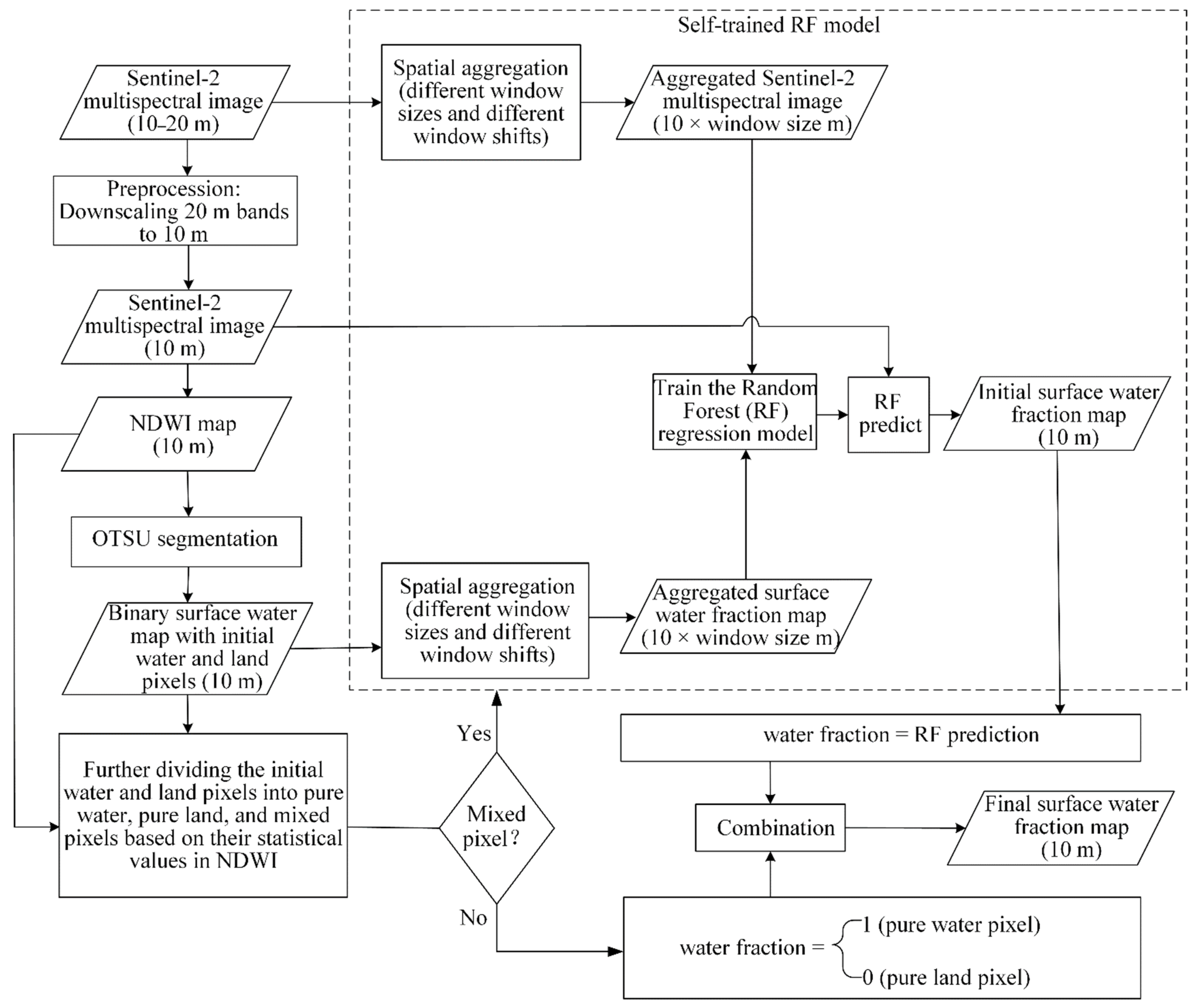
- AHSWFM uses a hierarchical structure that divides pixels into pure water, pure land and mixed water-land pixels, and predicts their water fractions separately to avoid overestimating the water fraction for pure land pixels and underestimating the water fraction for pure water pixels. Compared with the hierarchical surface water mapping method based on the linear mixture model [24,40], this study first explores the hierarchical strategy based on a random forest (RF) regression model to address the complicated water-land decomposition.
- AHSWFM is fully automated without any prior information or pre-defined thresholds. Compared with previous self-trained models that require training data or pre-defined thresholds to generate the binary water map used in the regression model, AHSWFM uses OTSU segmentation to automatically generate the water map in the regression model.
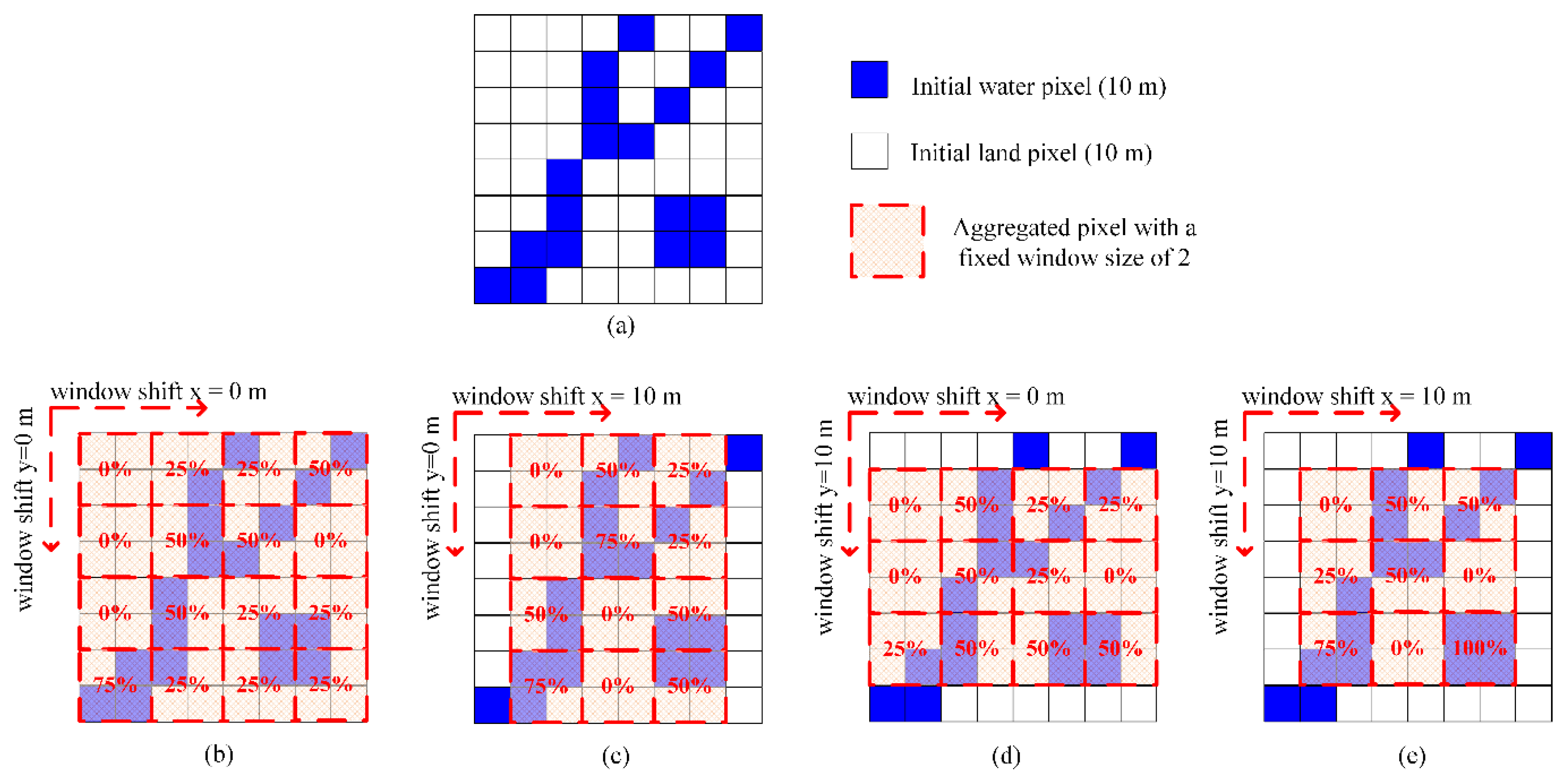
- The impacts of different window sizes and window shifts on the aggregation to coarse pixel samples in the water fraction regression are assessed.
2. Study Area and Data
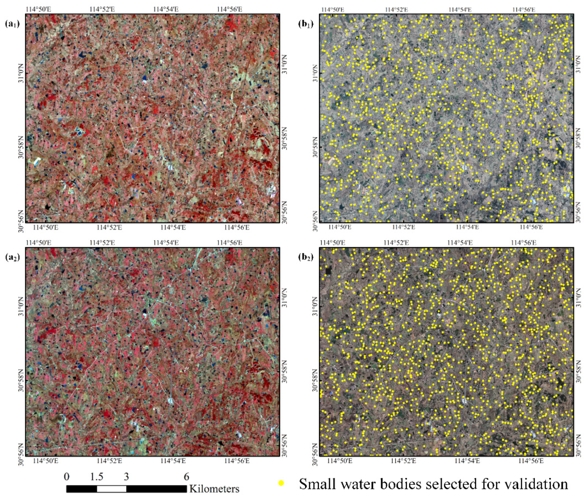
2.1. Study Area
2.2. Data
3. Methodology
3.1. Data Preprocessing
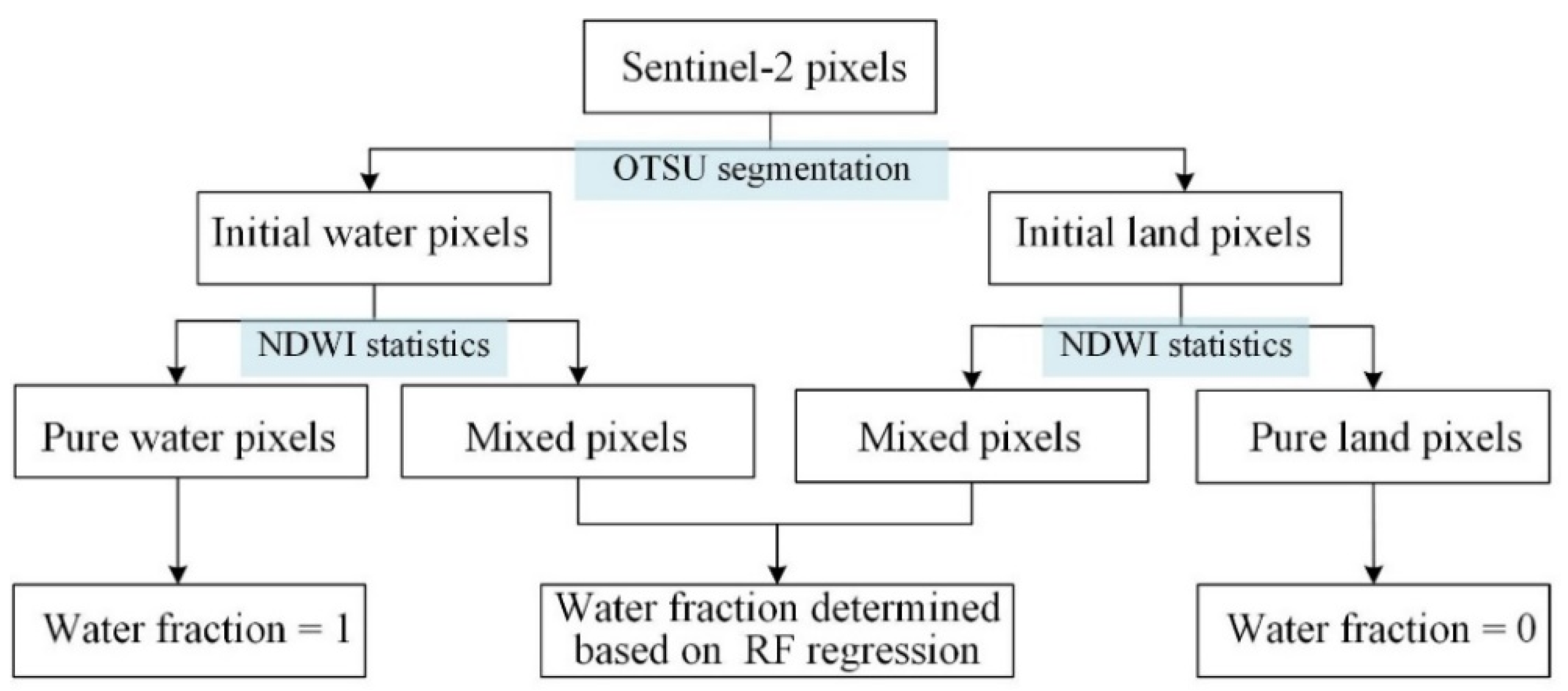
3.2. Producing the Initial 10 m Binary Surface Water Map Based on OTSU Segmentation
3.3. Generating the Pure Water, Pure Land and Mixed Pixels at 10 m Based on the Statistical Values in the NDWI
3.4. Self-Trained Regression and Hierarchical Prediction for the Final 10 m Surface Water Fraction Mapping Using RF
4. Experiment
4.1. Parameter Settings of AHSWFM
4.2. Methods for Comparison
4.3. Accuracy Assessment
5. Results
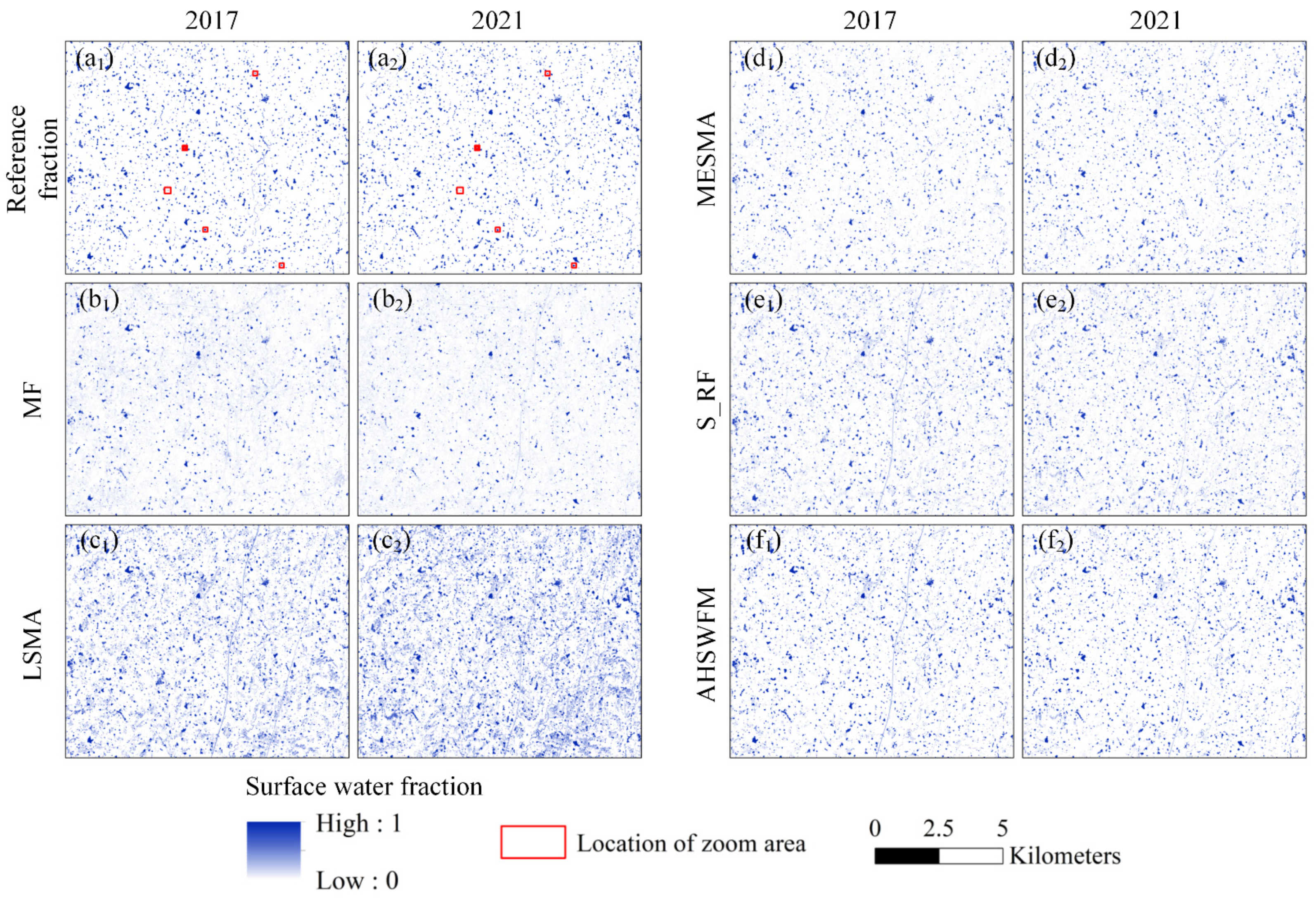
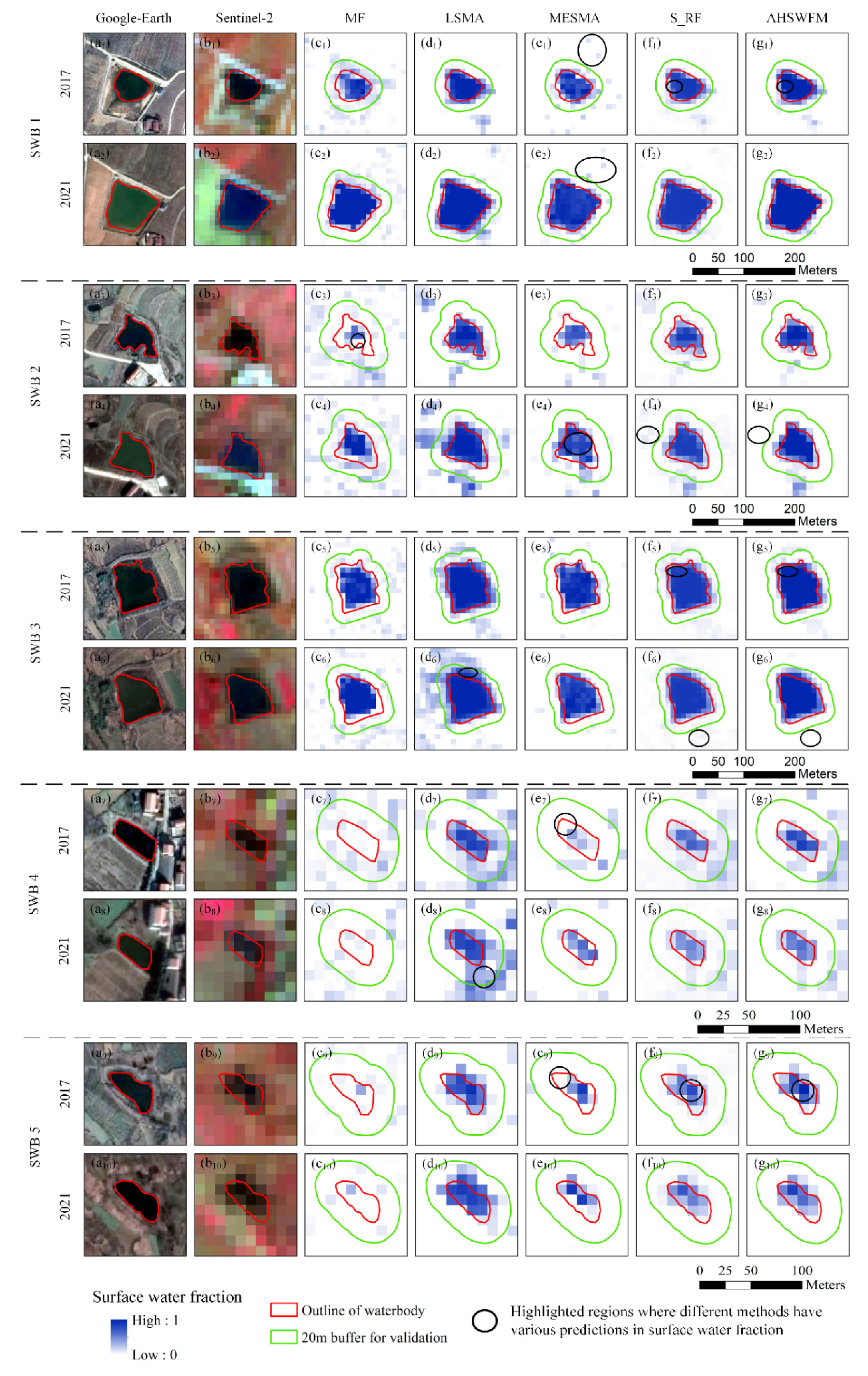
5.1. Visual Comparison of Different Water Fraction Maps
5.2. Accuracy Comparison of Different Water Fraction Maps
6. Discussion
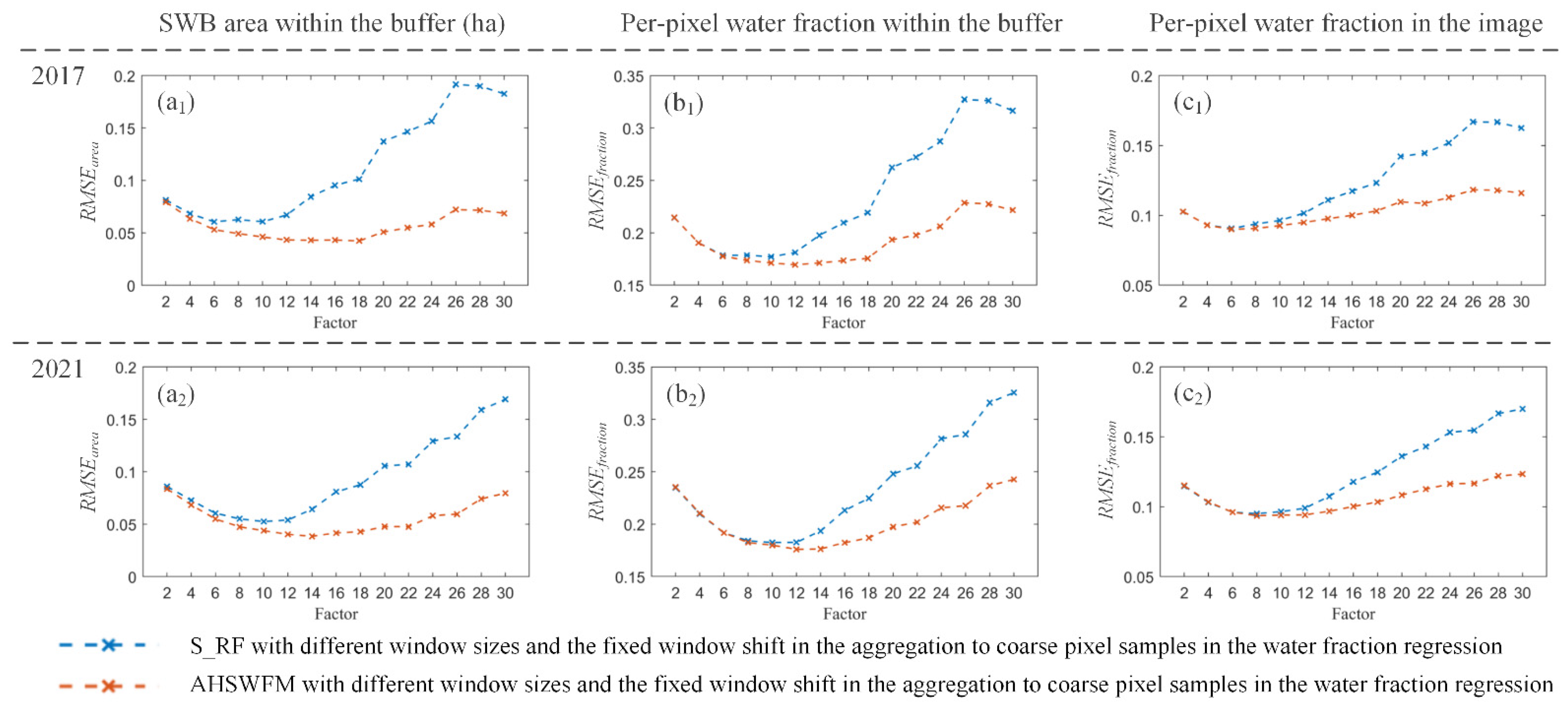
6.1. Impact of Different Window Sizes and Window Shifts in the Aggregation to Coarse Pixel Samples in the Water Fraction Regression on S_RF and AHSWFM
6.1.1. Impact of Different Window Sizes (and the Fixed Window Shift) in the Aggregation to Coarse Pixel Samples in the Water Fraction Regression on S_RF and AHSWFM
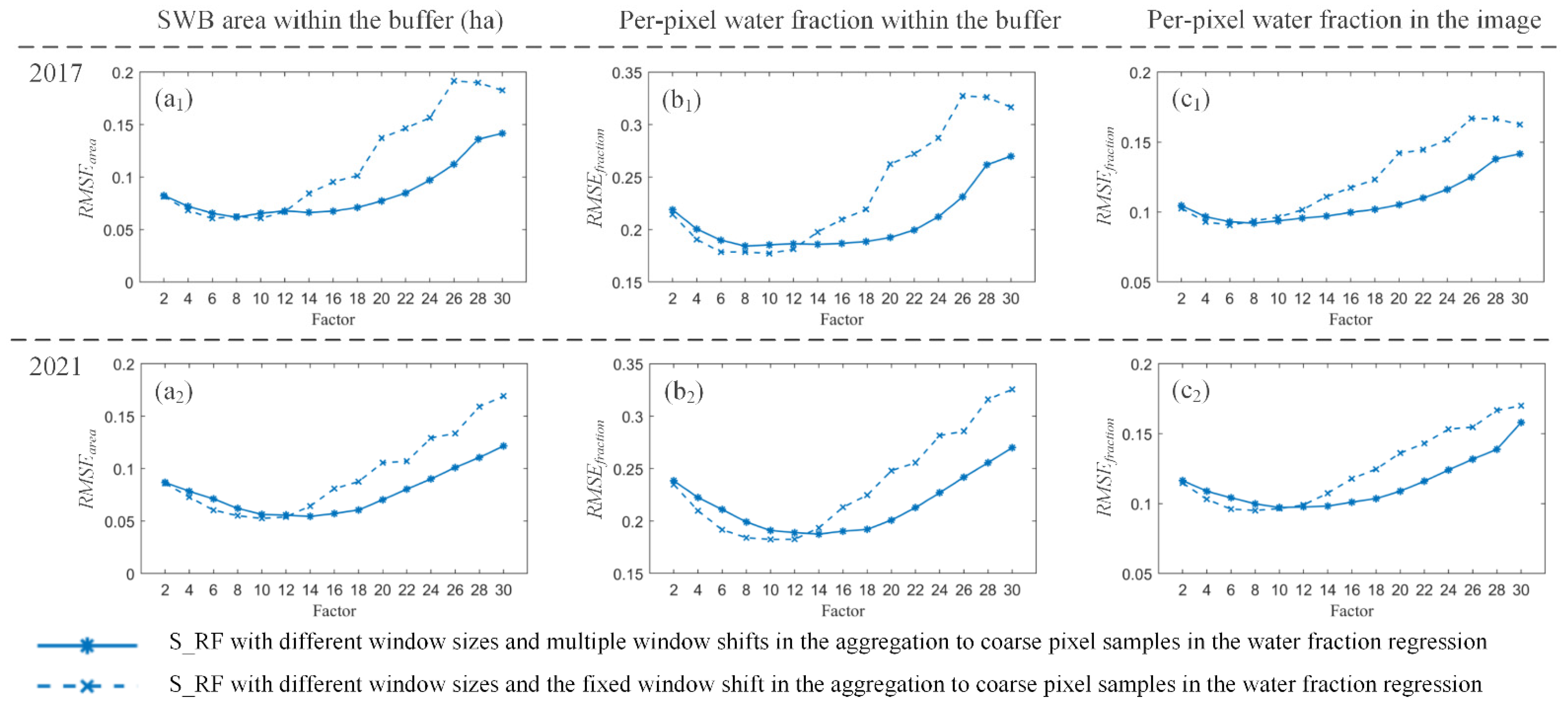
6.1.2. Impact of Different Window Sizes and Window Shifts in the Aggregation to Coarse Pixel Samples in the Water Fraction Regression on S_RF
6.1.3. Impact of Different Window Sizes and Window Shifts in the Aggregation to Coarse Pixel Samples in the Water Fraction Regression on AHSWFM
6.1.4. Comparison of Training Sample Number and Running Times of S_RF and AHSWFM
- When using the fixed window shift in producing regression samples, the increase of window size resulted in a decrease in sample numbers and running time. When the window size is too small, the samples may be not representative for the complex water-land composition. For example, if the window size is 2, when aggregating the 2 × 2 pixels from the binary water map to coarse pixel water fraction, only 5 values of coarse water fractions are obtained including 0% (none of the pixels labeled as water), 25% (1 pixel labeled as water), 50% (2 pixels labeled as water), 75% (3 pixels labeled as water) and 100% (all pixels labeled as water). Thus, both S_RF and AHSWFM with the window size of 2 generated high RMSE values in different metrics in Figure 10, Figure 11 and Figure 12. Considering the accuracies in Figure 10, Figure 11 and Figure 12 and the running times in Table 2, S_RF and AHSWFM with window sizes ranging from 6–10 can generate results with relatively high accuracy and low time cost.
- When using multiple shifts in producing the regression samples, the increasing of window size resulted in a decrease in sample numbers but not an obvious decrease in running time when the window size is larger than 2. For S_RF and AHSWFM, the running times are longer than 3100 s for the window size of 2, and are shorter than 1200 s for the other window sizes.
- The running time of S_RF and AHSWFM using multiple shifts are more than 10 times longer than those using fixed shift.
6.2. Limitations and Future Research
7. Conclusions
Author Contributions
Funding
Institutional Review Board Statement
Informed Consent Statement
Data Availability Statement
Acknowledgments
Conflicts of Interest
References
- Pekel, J.-F.; Cottam, A.; Gorelick, N.; Belward, A.S. High-resolution mapping of global surface water and its long-term changes. Nature 2016, 540, 418–422. [Google Scholar] [CrossRef] [PubMed]
- Downing, J.A.; Prairie, Y.; Cole, J.; Duarte, C.; Tranvik, L.; Striegl, R.G.; McDowell, W.; Kortelainen, P.; Caraco, N.; Melack, J. The global abundance and size distribution of lakes, ponds, and impoundments. Limnol. Oceanogr. 2006, 51, 2388–2397. [Google Scholar] [CrossRef] [Green Version]
- El Bilali, A.; Taghi, Y.; Briouel, O.; Taleb, A.; Brouziyne, Y. A framework based on high-resolution imagery datasets and MCS for forecasting evaporation loss from small reservoirs in groundwater-based agriculture. Agric. Water Manag. 2022, 262, 107434. [Google Scholar] [CrossRef]
- Perin, V.; Tulbure, M.G.; Gaines, M.D.; Reba, M.L.; Yaeger, M.A. A multi-sensor satellite imagery approach to monitor on-farm reservoirs. Remote Sens. Environ. 2022, 270, 112796. [Google Scholar] [CrossRef]
- Perin, V.; Tulbure, M.G.; Gaines, M.D.; Reba, M.L.; Yaeger, M.A. On-farm reservoir monitoring using Landsat inundation datasets. Agric. Water Manag. 2021, 246, 106694. [Google Scholar] [CrossRef]
- Habets, F.; Molénat, J.; Carluer, N.; Douez, O.; Leenhardt, D. The cumulative impacts of small reservoirs on hydrology: A review. Sci. Total Environ. 2018, 643, 850–867. [Google Scholar] [CrossRef] [Green Version]
- Downing, J.A. Emerging global role of small lakes and ponds: Little things mean a lot. Limnetica 2010, 29, 9–24. [Google Scholar] [CrossRef]
- Berg, M.D.; Popescu, S.C.; Wilcox, B.P.; Angerer, J.P.; Rhodes, E.C.; McAlister, J.; Fox, W.E. Small farm ponds: Overlooked features with important impacts on watershed sediment transport. J. Am. Water Resour. Assoc. 2016, 52, 67–76. [Google Scholar] [CrossRef]
- Pickens, A.H.; Hansen, M.C.; Hancher, M.; Stehman, S.V.; Tyukavina, A.; Potapov, P.; Marroquin, B.; Sherani, Z. Mapping and sampling to characterize global inland water dynamics from 1999 to 2018 with full Landsat time-series. Remote Sens. Environ. 2020, 243, 111792. [Google Scholar] [CrossRef]
- Li, X.; Ling, F.; Foody, G.M.; Boyd, D.S.; Jiang, L.; Zhang, Y.; Zhou, P.; Wang, Y.; Chen, R.; Du, Y. Monitoring high spatiotemporal water dynamics by fusing MODIS, Landsat, water occurrence data and DEM. Remote Sens. Environ. 2021, 265, 112680. [Google Scholar] [CrossRef]
- Guo, H.; He, G.; Jiang, W.; Yin, R.; Yan, L.; Leng, W. A multi-scale water extraction convolutional neural network (MWEN) method for GaoFen-1 remote sensing images. ISPRS Int. J. Geo-Inf. 2020, 9, 189. [Google Scholar] [CrossRef] [Green Version]
- Duan, Y.; Zhang, W.; Huang, P.; He, G.; Guo, H. A New Lightweight Convolutional Neural Network for Multi-Scale Land Surface Water Extraction from GaoFen-1D Satellite Images. Remote Sens. 2021, 13, 4576. [Google Scholar] [CrossRef]
- Zhan, W.; Chen, Y.; Zhou, J.; Wang, J.; Liu, W.; Voogt, J.; Zhu, X.; Quan, J.; Li, J. Disaggregation of remotely sensed land surface temperature: Literature survey, taxonomy, issues, and caveats. Remote Sens. Environ. 2013, 131, 119–139. [Google Scholar] [CrossRef]
- Li, X.; Ling, F.; Foody, G.M.; Ge, Y.; Zhang, Y.; Du, Y. Generating a series of fine spatial and temporal resolution land cover maps by fusing coarse spatial resolution remotely sensed images and fine spatial resolution land cover maps. Remote Sens. Environ. 2017, 196, 293–311. [Google Scholar] [CrossRef]
- Li, X.; Foody, G.M.; Boyd, D.S.; Ge, Y.; Zhang, Y.; Du, Y.; Ling, F. SFSDAF: An enhanced FSDAF that incorporates sub-pixel class fraction change information for spatio-temporal image fusion. Remote Sens. Environ. 2020, 237, 111537. [Google Scholar] [CrossRef]
- Thenkabail, P. Remote Sensing Handbook—Three Volume Set; CRC Press: Boca Raton, FL, USA, 2018. [Google Scholar]
- Ottinger, M.; Bachofer, F.; Huth, J.; Kuenzer, C. Mapping Aquaculture Ponds for the Coastal Zone of Asia with Sentinel-1 and Sentinel-2 Time Series. Remote Sens. 2022, 14, 153. [Google Scholar] [CrossRef]
- Kaplan, G.; Avdan, U. Object-based water body extraction model using Sentinel-2 satellite imagery. Eur. J. Remote Sens. 2017, 50, 137–143. [Google Scholar] [CrossRef] [Green Version]
- Bie, W.; Fei, T.; Liu, X.; Liu, H.; Wu, G. Small water bodies mapped from Sentinel-2 MSI (MultiSpectral Imager) imagery with higher accuracy. Int. J. Remote Sens. 2020, 41, 7912–7930. [Google Scholar] [CrossRef]
- Du, Y.; Zhang, Y.; Ling, F.; Wang, Q.; Li, W.; Li, X. Water bodies’ mapping from Sentinel-2 imagery with modified normalized difference water index at 10-m spatial resolution produced by sharpening the SWIR band. Remote Sens. 2016, 8, 354. [Google Scholar] [CrossRef] [Green Version]
- Freitas, P.; Vieira, G.; Canário, J.; Folhas, D.; Vincent, W.F. Identification of a threshold minimum area for reflectance retrieval from thermokarst lakes and ponds using full-pixel data from Sentinel-2. Remote Sens. 2019, 11, 657. [Google Scholar] [CrossRef] [Green Version]
- Hu, Y.H.; Lee, H.; Scarpace, F. Optimal linear spectral unmixing. IEEE Trans. Geosci. Remote Sens. 1999, 37, 639–644. [Google Scholar] [CrossRef]
- Quintano, C.; Fernández-Manso, A.; Shimabukuro, Y.E.; Pereira, G. Spectral unmixing. Int. J. Remote Sens. 2012, 33, 5307–5340. [Google Scholar] [CrossRef]
- Ma, B.; Wu, L.; Zhang, X.; Li, X.; Liu, Y.; Wang, S. Locally adaptive unmixing method for lake-water area extraction based on MODIS 250 m bands. Int. J. Appl. Earth Obs. Geoinf. 2014, 33, 109–118. [Google Scholar] [CrossRef]
- Keshava, N.; Mustard, J.F. Spectral unmixing. IEEE Signal Process. Mag. 2002, 19, 44–57. [Google Scholar] [CrossRef]
- Heinz, D.C. Fully constrained least squares linear spectral mixture analysis method for material quantification in hyperspectral imagery. IEEE Trans. Geosci. Remote Sens. 2001, 39, 529–545. [Google Scholar] [CrossRef] [Green Version]
- Ling, F.; Li, X.; Foody, G.M.; Boyd, D.; Ge, Y.; Li, X.; Du, Y. Monitoring surface water area variations of reservoirs using daily MODIS images by exploring sub-pixel information. ISPRS J. Photogramm. Remote Sens. 2020, 168, 141–152. [Google Scholar] [CrossRef]
- Xiong, L.; Deng, R.; Li, J.; Liu, X.; Qin, Y.; Liang, Y.; Liu, Y. Subpixel surface water extraction (SSWE) using Landsat 8 OLI data. Water 2018, 10, 653. [Google Scholar] [CrossRef] [Green Version]
- Xie, H.; Luo, X.; Xu, X.; Pan, H.; Tong, X. Automated subpixel surface water mapping from heterogeneous urban environments using Landsat 8 OLI imagery. Remote Sens. 2016, 8, 584. [Google Scholar] [CrossRef] [Green Version]
- Ray, T.W.; Murray, B.C. Nonlinear spectral mixing in desert vegetation. Remote Sens. Environ. 1996, 55, 59–64. [Google Scholar] [CrossRef]
- De Vries, B.; Huang, C.; Lang, M.W.; Jones, J.W.; Huang, W.; Creed, I.F.; Carroll, M.L. Automated quantification of surface water inundation in wetlands using optical satellite imagery. Remote Sens. 2017, 9, 807. [Google Scholar] [CrossRef] [Green Version]
- Sun, W.; Du, B.; Xiong, S. Quantifying sub-pixel surface water coverage in urban environments using low-albedo fraction from Landsat imagery. Remote Sens. 2017, 9, 428. [Google Scholar] [CrossRef] [Green Version]
- Franke, J.; Roberts, D.A.; Halligan, K.; Menz, G. Hierarchical multiple endmember spectral mixture analysis (MESMA) of hyperspectral imagery for urban environments. Remote Sens. Environ. 2009, 113, 1712–1723. [Google Scholar] [CrossRef]
- Jarchow, C.J.; Sigafus, B.H.; Muths, E.; Hossack, B.R. Using full and partial unmixing algorithms to estimate the inundation extent of small, isolated stock ponds in an arid landscape. Wetlands 2020, 40, 563–575. [Google Scholar] [CrossRef]
- Sall, I.; Jarchow, C.J.; Sigafus, B.H.; Eby, L.A.; Forzley, M.J.; Hossack, B.R. Estimating inundation of small waterbodies with sub-pixel analysis of Landsat imagery: Long-term trends in surface water area and evaluation of common drought indices. Remote Sens. Ecol. Conserv. 2021, 7, 109–124. [Google Scholar] [CrossRef]
- Li, L.; Vrieling, A.; Skidmore, A.; Wang, T.; Turak, E. Monitoring the dynamics of surface water fraction from MODIS time series in a Mediterranean environment. Int. J. Appl. Earth Obs. Geoinf. 2018, 66, 135–145. [Google Scholar] [CrossRef]
- Li, L.; Skidmore, A.; Vrieling, A.; Wang, T. A new dense 18-year time series of surface water fraction estimates from MODIS for the Mediterranean region. Hydrol. Earth Syst. Sci. 2019, 23, 3037–3056. [Google Scholar] [CrossRef] [Green Version]
- Liang, J.; Liu, D. Automated estimation of daily surface water fraction from MODIS and Landsat images using Gaussian process regression. Int. J. Remote Sens. 2021, 42, 4261–4283. [Google Scholar] [CrossRef]
- Rover, J.; Wylie, B.K.; Ji, L. A self-trained classification technique for producing 30 m percent-water maps from Landsat data. Int. J. Remote Sens. 2010, 31, 2197–2203. [Google Scholar] [CrossRef]
- Luo, X.; Xie, H.; Xu, X.; Pan, H.; Tong, X. A hierarchical processing method for subpixel surface water mapping from highly heterogeneous urban environments using Landsat OLI data. In Proceedings of the 2016 IEEE International Geoscience and Remote Sensing Symposium (IGARSS), Beijing, China, 10–15 July 2016; pp. 6221–6224. [Google Scholar]
- Jiang, W.; Ni, Y.; Pang, Z.; Li, X.; Ju, H.; He, G.; Lv, J.; Yang, K.; Fu, J.; Qin, X. An effective water body extraction method with new water index for sentinel-2 imagery. Water 2021, 13, 1647. [Google Scholar] [CrossRef]
- Jiang, H.; Wang, M.; Hu, H.; Xu, J. Evaluating the Performance of Sentinel-1A and Sentinel-2 in Small Waterbody Mapping over Urban and Mountainous Regions. Water 2021, 13, 945. [Google Scholar] [CrossRef]
- Yu, Z.; Di, L.; Rahman, M.; Tang, J. Fishpond mapping by spectral and spatial-based filtering on google earth engine: A case study in singra upazila of Bangladesh. Remote Sens. 2020, 12, 2692. [Google Scholar] [CrossRef]
- Yang, X.; Zhao, S.; Qin, X.; Zhao, N.; Liang, L. Mapping of urban surface water bodies from Sentinel-2 MSI imagery at 10 m resolution via NDWI-based image sharpening. Remote Sens. 2017, 9, 596. [Google Scholar] [CrossRef] [Green Version]
- Wang, Z.; Liu, J.; Li, J.; Zhang, D.D. Multi-spectral water index (MuWI): A native 10-m multi-spectral water index for accurate water mapping on Sentinel-2. Remote Sens. 2018, 10, 1643. [Google Scholar] [CrossRef] [Green Version]
- Aspinall, R.J.; Marcus, W.A.; Boardman, J.W. Considerations in collecting, processing, and analysing high spatial resolution hyperspectral data for environmental investigations. J. Geogr. Syst. 2002, 4, 15–29. [Google Scholar] [CrossRef]
- Sun, G.; Huang, H.; Weng, Q.; Zhang, A.; Jia, X.; Ren, J.; Sun, L.; Chen, X. Combinational shadow index for building shadow extraction in urban areas from Sentinel-2A MSI imagery. Int. J. Appl. Earth Obs. Geoinf. 2019, 78, 53–65. [Google Scholar] [CrossRef]
- Kwarteng, P.; Chavez, A. Extracting spectral contrast in Landsat Thematic Mapper image data using selective principal component analysis. Photogramm. Eng. Remote Sens. 1989, 55, 339–348. [Google Scholar]
- McFeeters, S.K. The use of the Normalized Difference Water Index (NDWI) in the delineation of open water features. Int. J. Remote Sens. 1996, 17, 1425–1432. [Google Scholar] [CrossRef]
- Otsu, N. A threshold selection method from gray-level histograms. IEEE Trans. Syst. Man Cybern. 1979, 9, 62–66. [Google Scholar] [CrossRef] [Green Version]
- Foroosh, H.; Zerubia, J.B.; Berthod, M. Extension of phase correlation to subpixel registration. IEEE Trans. Image Process. 2002, 11, 188–200. [Google Scholar] [CrossRef] [Green Version]
- Zhou, Y.; Luo, J.; Shen, Z.; Hu, X.; Yang, H. Multiscale water body extraction in urban environments from satellite images. IEEE J. Sel. Top. Appl. Earth Obs. Remote Sens. 2014, 7, 4301–4312. [Google Scholar] [CrossRef]
- Halabisky, M.; Moskal, L.M.; Gillespie, A.; Hannam, M. Reconstructing semi-arid wetland surface water dynamics through spectral mixture analysis of a time series of Landsat satellite images (1984–2011). Remote Sens. Environ. 2016, 177, 171–183. [Google Scholar] [CrossRef]
- Van Der Meer, F. Iterative spectral unmixing (ISU). Int. J. Remote Sens. 1999, 20, 3431–3436. [Google Scholar] [CrossRef]
- Feyisa, G.L.; Meilby, H.; Fensholt, R.; Proud, S.R. Automated Water Extraction Index: A new technique for surface water mapping using Landsat imagery. Remote Sens. Environ. 2014, 140, 23–35. [Google Scholar] [CrossRef]
- Xu, H. Modification of normalised difference water index (NDWI) to enhance open water features in remotely sensed imagery. Int. J. Remote Sens. 2006, 27, 3025–3033. [Google Scholar] [CrossRef]
- Xu, H. A study on information extraction of water body with the modified normalized difference water index (MNDWI). J. Remote Sens. 2005, 9, 589–595. [Google Scholar]
- Zhang, J.; Zhang, Q.; Bao, A.; Wang, Y. A new remote sensing dryness index based on the near-infrared and red spectral space. Remote Sens. 2019, 11, 456. [Google Scholar] [CrossRef] [Green Version]
- Yang, Y.; Liu, Y.; Zhou, M.; Zhang, S.; Zhan, W.; Sun, C.; Duan, Y. Landsat 8 OLI image based terrestrial water extraction from heterogeneous backgrounds using a reflectance homogenization approach. Remote Sens. Environ. 2015, 171, 14–32. [Google Scholar] [CrossRef]
- Misra, G.; Cawkwell, F.; Wingler, A. Status of phenological research using Sentinel-2 data: A review. Remote Sens. 2020, 12, 2760. [Google Scholar] [CrossRef]
- Markert, K.N.; Markert, A.M.; Mayer, T.; Nauman, C.; Haag, A.; Poortinga, A.; Bhandari, B.; Thwal, N.S.; Kunlamai, T.; Chishtie, F. Comparing sentinel-1 surface water mapping algorithms and radiometric terrain correction processing in southeast asia utilizing google earth engine. Remote Sens. 2020, 12, 2469. [Google Scholar] [CrossRef]
- Ludwig, C.; Walli, A.; Schleicher, C.; Weichselbaum, J.; Riffler, M. A highly automated algorithm for wetland detection using multi-temporal optical satellite data. Remote Sens. Environ. 2019, 224, 333–351. [Google Scholar] [CrossRef]
- Yuan, X.; Wu, L.; Peng, Q. An improved Otsu method using the weighted object variance for defect detection. Appl. Surf. Sci. 2015, 349, 472–484. [Google Scholar] [CrossRef] [Green Version]


| Method | MF | LSMA | MESMA | S_RF | AHSWFM | ||
|---|---|---|---|---|---|---|---|
| RMSEarea: RMSE in SWB area within the buffer (ha) | 2017 | 0.0938 | 0.0517 | 0.0845 | 0.0608 | 0.0461 | |
| 2021 | 0.1065 | 0.0873 | 0.0592 | 0.0526 | 0.0440 | ||
| RMSEfraction: RMSE in per-pixel water fraction | Within the buffer | 2017 | 0.2679 | 0.1785 | 0.2119 | 0.1772 | 0.1714 |
| 2021 | 0.2765 | 0.2188 | 0.1959 | 0.1826 | 0.1799 | ||
| In the image | 2017 | 0.1336 | 0.1327 | 0.1055 | 0.0964 | 0.0926 | |
| 2021 | 0.1416 | 0.1618 | 0.1018 | 0.0965 | 0.0940 | ||
| Window Size | Fixed Window Shift | Multiple Window Shifts | ||||
|---|---|---|---|---|---|---|
| Number of Training Samples | Running Time (Second) | Number of Training Samples | Running Time (Second) | |||
| S_RF | AHSWFM | S_RF | AHSWFM | |||
| 2 | 331,992 | 1419.7 | 1420.0 | 1,325,653 | 3102.0 | 3102.2 |
| 4 | 82,998 | 125.6 | 125.8 | 1,321,029 | 1203.3 | 1203.5 |
| 6 | 36,888 | 103.6 | 104.0 | 1,316,413 | 1075.8 | 1075.9 |
| 8 | 20,670 | 94.8 | 95.0 | 1,311,805 | 1036.0 | 1036.2 |
| 10 | 13,208 | 89.1 | 89.3 | 1,307,205 | 1018.9 | 1019.0 |
| 12 | 9222 | 84.6 | 84.8 | 1,302,613 | 1022.8 | 1022.9 |
| 14 | 6660 | 81.4 | 81.5 | 1,298,029 | 1047.0 | 1047.1 |
| 16 | 5135 | 79.1 | 79.3 | 1,293,453 | 1069.0 | 1069.2 |
| 18 | 4060 | 77.0 | 77.2 | 1,288,885 | 1092.2 | 1092.3 |
| 20 | 3276 | 75.4 | 75.6 | 1,284,325 | 1110.6 | 1111.1 |
| 22 | 2679 | 74.4 | 74.5 | 1,279,773 | 1129.6 | 1129.8 |
| 24 | 2279 | 72.6 | 72.8 | 1,275,229 | 1149.3 | 1149.5 |
| 26 | 1920 | 68.1 | 68.2 | 1,270,693 | 1178.9 | 1179.0 |
| 28 | 1665 | 59.8 | 60.0 | 1,266,165 | 1200.0 | 1200.2 |
| 30 | 1428 | 59.1 | 59.2 | 1,261,645 | 1228.4 | 1228.6 |
Publisher’s Note: MDPI stays neutral with regard to jurisdictional claims in published maps and institutional affiliations. |
© 2022 by the authors. Licensee MDPI, Basel, Switzerland. This article is an open access article distributed under the terms and conditions of the Creative Commons Attribution (CC BY) license (https://creativecommons.org/licenses/by/4.0/).
Share and Cite
Wang, Y.; Li, X.; Zhou, P.; Jiang, L.; Du, Y. AHSWFM: Automated and Hierarchical Surface Water Fraction Mapping for Small Water Bodies Using Sentinel-2 Images. Remote Sens. 2022, 14, 1615. https://doi.org/10.3390/rs14071615
Wang Y, Li X, Zhou P, Jiang L, Du Y. AHSWFM: Automated and Hierarchical Surface Water Fraction Mapping for Small Water Bodies Using Sentinel-2 Images. Remote Sensing. 2022; 14(7):1615. https://doi.org/10.3390/rs14071615
Chicago/Turabian StyleWang, Yalan, Xiaodong Li, Pu Zhou, Lai Jiang, and Yun Du. 2022. "AHSWFM: Automated and Hierarchical Surface Water Fraction Mapping for Small Water Bodies Using Sentinel-2 Images" Remote Sensing 14, no. 7: 1615. https://doi.org/10.3390/rs14071615
APA StyleWang, Y., Li, X., Zhou, P., Jiang, L., & Du, Y. (2022). AHSWFM: Automated and Hierarchical Surface Water Fraction Mapping for Small Water Bodies Using Sentinel-2 Images. Remote Sensing, 14(7), 1615. https://doi.org/10.3390/rs14071615