Ice Detection with Sentinel-1 SAR Backscatter Threshold in Long Sections of Temperate Climate Rivers

Abstract

Climate change leads to more variable meteorological conditions. In many Northern Hemisphere temperate regions, cold seasons have become more variable and unpredictable, necessitating frequent river ice observations over long sections of rivers. Satellite SAR (Synthetic Aperture Radar)-based river ice detection models have been successfully applied and tested, but different hydrological, morphological and climatological conditions can affect their skill. In this study, we developed and tested Sentinel-1 SAR-based ice detection models in 525 km sections of the Nemunas and Neris Rivers. We analyzed three binary classification models based on VV, VH backscatter and logistic regression. The model sensitivity and specificity were used to determine the optimal threshold between ice and water classes. We used in situ observations and Sentinel-2 Sen2Cor ice mask to validate models in different ice conditions. In most cases, SAR-based ice detection models outperformed Sen2Cor classification because Sen2Cor misclassified pixels as ice in areas with translucent clouds, undetected by the scene classification algorithm, and misclassified pixels as water in cloud or river valley shadow. SAR models were less accurate in river sections where river flow and ice formation conditions were affected by large valley-dammed reservoirs. Sen2Cor and SAR models accurately detected border and consolidated ice but were less accurate in moving ice conditions. The skill of models depended on how dense the moving ice was. With a lowered classification threshold and increased model sensitivity, SAR models detected sparse frazil ice. In most cases, the VV polarization-based model was more accurate than the VH polarization-based model. The results of logistic and VV models were highly correlated, and the use of VV was more constructive due to its simpler algorithm.

1. Introduction

River ice is an important factor in biological, physical and chemical processes in higher-latitude regions. Climate change has drastically altered ice formation, as well as decay times and dates, around the globe [1,2,3]. These changes create various challenges for the economic sectors [4] and civilian lives. Ice creates operational constraints that hinder power production in hydropower systems. River ice can cause flooding, damage structures such as culverts and bridges, disturb water transportation or block water supply. Ice surfaces influence local air temperature and humidity, and smaller frozen rivers have a lower discharge and modified redistribution of water [5]. These factors make ice cover monitoring an important task.

In recent years, the cold season has become more unpredictable with the frequent variation of air temperature. Consequently, the river ice extent and types are often altered throughout the winter. Due to frequent temperature fluctuations in the cold season, ice cover forms and melts away several times a year. Therefore, the consistent monitoring of river ice is much more important than in the past when ice formation and decay were more predictable.

In some regions, ground-based freshwater ice observations are scarce due to inaccessible remote locations or limited available resources. The global reduction of ground-based freshwater ice observations began in the 1980s [6] and has further decreased due to the introduction of automatic gauges.

Large-scale in situ observations require considerable human and financial resources. Therefore, satellite imagery is likely the best alternative to monitor ice formation in rivers. Satellite remote sensing with large spatial coverage and frequent revisit time is a robust addition to the in situ monitoring of freshwater ice. Satellite-based studies aim to determine ice extent, ice phenology and ice types. The variety of ice types and their distribution highly depend on meteorological conditions, river channel properties and hydrology [7]. For example, the Peace River in Canada has sections of rapids and falls that are responsible for the large variety of ice cover types found there. Meanwhile, the Vistula River in Poland has a slower flow and more homogenous riverbed. Therefore, its ice cover during winter is also more homogenous [8]. The number of identified ice types varies. In most studies, thermal ice, frazil ice and consolidated ice types are ignored [9], while in other studies, smooth clear ice, drifting frazil pans, dense moving ice floes and agglomerated ice types are included [10].

SAR (Synthetic Aperture Radar) data have relatively a high resolution and are almost unaffected by cloud cover. Consequently, SAR data are is typically used in river ice monitoring. The SAR backscatter from water and ice is distinct because of the difference in roughness and dielectric properties. Rough ice surfaces usually have the highest backscatter values, making, it is easy to identify consolidated ice [11] and agglomerated ice [8], while newly formed ice has similar backscatter values to open water [12], making it harder to identify. Differentiating rapids from ice are also problematic [13]. In addition to providing information about surface roughness, SAR is also capable of providing information about volume scattering. Volume scattering is dependent on the size, shape and density of air inclusions within the ice cover, and the interface between the ice layer and water [10]. In the case of an ice jam, ice layers are stacked, causing multiple scattering between these layers [14]. However, the main scattering mechanism of river ice is normally surface scattering rather than volume scattering, except in the case of consolidated or thick, porous ice [15]. Wet snow significantly reduces the accuracy of ice monitoring. Therefore, some errors may occur when analyzing ice cover types under wet snow cover [9]. There is a high correlation between snow cover wetness and the visibility of ice cover underneath it [16]. When the snow cover is thick, ice cover interpretations become highly subjective. It is only possible to separate very rough and smooth ice cover, but even then, the possibility of error remains high [10]. Most freshwater ice studies have been based on RADARSAT 1–2 satellites [6,8,11,15,17,18] and performed in middle and higher latitudes of North America. To date, only several river ice studies have used Sentinel-1 SAR data for river ice monitoring [16,19,20,21]. The wide swath, high spatial resolution and short revisit time in high latitudes [8] determine the high application potential of these data in river ice studies.

It is particularly challenging to validate river ice products, as in most locations, in situ river ice data are available only for small river sections near hydrological stations. Validation from aerial photos can provide information about ice extent and types. However, the spatial coverage and frequency of aerial photos in most regions are scarce. Multispectral satellite data have been used for ice detection since the end of 20^th century. The high temporal resolution of Moderate Resolution Imaging Spectroradiometer (MODIS) on Terra and Aqua NASA satellites provides an opportunity to observe the landscape daily. However, their low spatial resolution limits observations to only large objects, such as seas [22], large lakes [23] and large rivers [24]. In this case, a careful identification of mixed pixels that contain both water and land is needed [25,26]. Landsat satellites provide a finer spatial resolution, but their low temporal resolution may not allow for the observation of ice freeze and break-up dates [23]. The Landsat data archive provides an opportunity for long-term analysis [27].

Ice has a higher reflectance in visible bands than water. Therefore, it is distinguishable using spectral indices that use visible and shortwave infrared (SWIR) bands. The Normalized Difference Snow Index (NDSI) was used to map snow- and ice-covered areas in high-latitude regions from Landsat Thematic Mapper (TM) and Enhanced Thematic Mapper+ (ETM+) scenes [28]. Li et al. [27] validated the NDSI with green and SWIR bands to detect river ice in high altitudes in the Tibetan Plateau.

Clouds are the main problem of optical remote sensing, as they substantially reduce the usability of images. Clouds are very prominent in northern regions, such as Lithuania, where often there might be only several cloud-free images during the winter season. Good cloud masking is needed to use partly cloudy images [28]. With more and more instruments in orbit, the use of multisource data becomes an advantage that has been proven to provide better results. In addition, webcams or crowdsourcing can be used as other complementary sources of data [23,29].

The Copernicus Land Monitoring Service (CLMS) provides high-resolution (20 m × 20 m) River and Lake Ice Extent (RLIE) products based on Sentinel-1 and Sentinel-2 satellite imagery. The accuracy of the RLIE S2 product, which uses Sentinel-2 data, is higher than 85% for rivers and lakes [30]. The accuracy assessment was performed using in situ data from the Czech Republic, Finland, Hungary and Serbia, as well as the visual analysis of optical remote sensing images. The products based on Sentinel-1 data (RLIE S1) and the combination of Sentinel-1 and Sentinel-2 (RLIE S1 + S2) are still being validated.

In this study, we tested the ability of Sentinel-1 SAR data to detect ice extent in two major Lithuanian rivers: the Nemunas and Neris Rivers. The application of river ice remote sensing in these relatively narrow (width: 80–300 m) and shallow rivers added further challenges related to backscatter interaction with vegetation, river bottom and shadowing by steep valley slopes. The understanding of SAR signal interaction with river ice remains incomplete [21,31]. Therefore, the local hydrological, morphological and climatic conditions might affect the accuracy of developed ice detection models and validation for other rivers. We analyzed long sections of the Nemunas (290 km) and Neris (235 km) Rivers with different hydrological and morphological conditions. SAR data are more viable for ice extent monitoring in this region than optical remote sensing images due to almost permanent cloud cover during the cold season in Lithuania. We used the backscatter intensity threshold method to detect pixels with ice in the rivers, and used in situ observation and Sentinel-2 Multispectral Imager (MSI) data to validate the accuracy of river ice detection.

This study aims to provide an understanding of the application of Sentinel-1 SAR data for monitoring the extent of river ice. The main objective of this study was to evaluate the potential of SAR data to detect river ice in long sections of narrow rivers. Second, we tested the efficiency of classification threshold optimization using model sensitivity and specificity. Subsequently, we validated ice detection models in diverse ice conditions and described the potential sources of uncertainties.

2. Materials and Methods

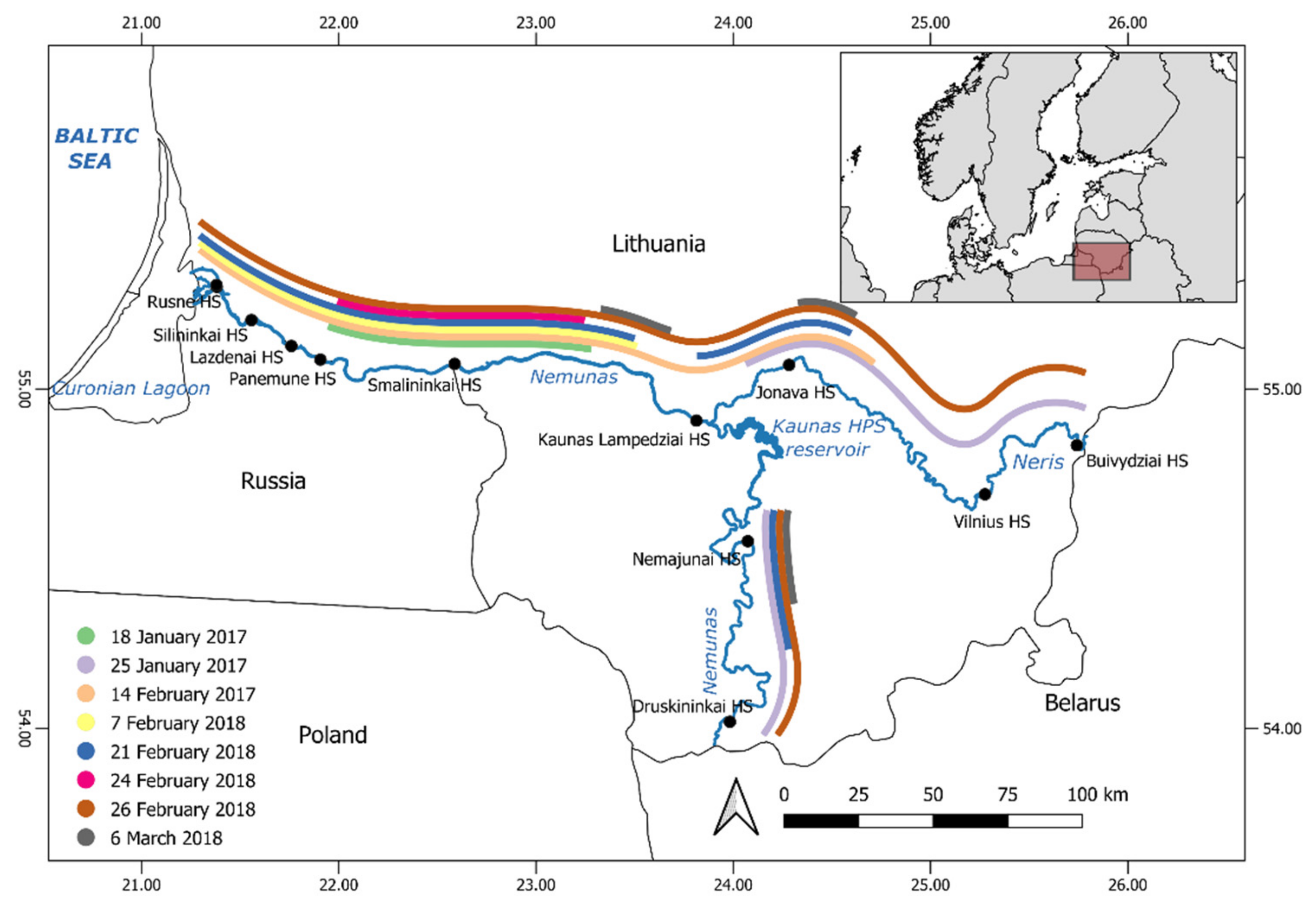
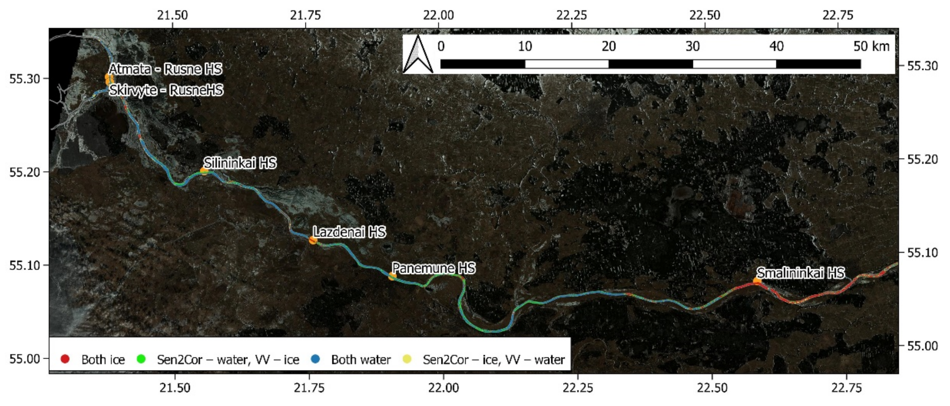
2.1. Study Area

Even a relatively high resolution of Sentinel-1 SAR IW GRD products limits the application of river ice detection algorithms in narrow rivers. Consequently, for this study, we chose two major Lithuanian rivers: the Nemunas and Neris Riers (Figure 1). We studied ice in the Lithuanian part of these rivers due to data availability for validation from the Lithuanian Hydrometeorological Service hydrological stations.

The Nemunas and Neris Rivers are lowland rivers, reaching up to 200 m in width for most of their sections, and the width can exceed 300 m only in some places. At the Nemunas River downstream from the Smalininkai hydrological station (HS), the river width is larger and can reach 500 m. These rivers are shallow and have several islands and shoals. We used river polygons from the national georeferenced base of cadastral data at scale 1:10,000 to delineate the riverbanks.

In the initial analysis of backscatter during winter, we found that due to different ice formation conditions, the backscatter from ice in the valley-dammed Kaunas hydropower station (HPS) Reservoir was different from the ice backscatter in other parts of the river. This difference was most likely caused by the reduced flow speed and thermal stratification in the reservoir. Consequently, we excluded the 50 km-long Nemunas River section upstream from the Kaunas HP dam from further analyses.

2.2. Model Development and Validation

Depending on the stage and conditions of freezing and break-up, ice in rivers can consist of different types. These types range from frazil slush and frazil pans to large ice pans and consolidated ice cover. The boundaries between ice forms are fuzzy and subjective. Thus, the confident differentiation of river ice types is challenging, even when observing on the ground. This task is more challenging using remote sensing. Therefore, we aimed to study the ability of SAR to detect ice extent without the differentiation of ice types. On the other hand, we used in situ observations in hydrological stations to evaluate the skill of classification models to detect different types of ice.

We used binary classification with water and ice classes for ice extent detection. The binary classification is mostly effective when the same class covers the whole pixel, which was an uncommon case in the rather narrow and shallow rivers that we studied. In frequent cases with frazil ice and ice pans, the pixel backscatter values can be a combination of signals from ice and water surfaces. We used such cases to estimate the ability of the Sentinel-1 SAR to detect the ice signal, even in pixels that covered a mixture of ice and open water surfaces.

We developed classification models using VH and VV polarization backscatter intensity, as well as the logistic model, to determine the river ice extent. VH and VV classification models are the thresholds of the backscatter values in the respective polarizations. The logistic regression model linearly combines the VV and VH polarizations:

log(p/(1 − p)) = β₀ + β_VV × VV_Sigma0 + β_VH × VH_Sigma0,

(1)

where p is the probability of ice; VV_Sigma0 and VH_Sigma0 are the scattering coefficient values in the VV and VH polarizations; and β₀, β_VV and β_VH are the model parameters.

We used two ground truth sources for the development and validation of the river ice detection models: (1) in situ observations of ice types in hydrological stations, and (2) Sentinel-2 MSI ice extent estimated using the Sen2Cor processor.

In situ information on ice types in all 11 hydrological stations (Figure 1) located on Nemunas and Neris Rivers was collected form the Lithuanian Hydrometeorological Service archives. The classes describing the in situ ice conditions in hydrological stations were: open water, border ice, sparse or dense frazil ice, sparse or dense ice pans, consolidated ice, consolidated ice with open water areas, and ice jams upstream or downstream from hydrological station. The differentiation of ice types is subjective, but it represents the most reliable aggregated information on ice conditions in the field of view of the observer. Thus, we considered this information on river ice as the most reliable representation of the ground truth. In situ observations represent only small river areas in the field of the observer. To obtain information on ice conditions in other parts of the rivers, we used the Sen2Cor ice mask based on Sentinel-2 MSI data. Sen2Cor scene classification uses a series of threshold tests that use reflectance from the Sentinel-2 spectral bands. In addition, thresholds are applied on band ratios and radiometric indexes. Snow and ice masks are distinguished using the NDSI (Normalized Difference Snow Index).

2.3. Satellite Data

The data of in situ ice observations, as well as water and air temperature, were used to determine the beginning and end of the ice seasons. We looked for matchups (within a 24 h window) between the Sentinel-1 SAR IW GRD High-Resolution and Sentinel-2 MSI Level1C acquisitions during the 2015–2019 cold seasons. The cloud cover in the Sentinel-2 images significantly limited the number of matchups. Due to frequent overcast conditions in the analyzed region in winter and early spring, we used Sentinel-2 images with cloud cover or cloud shadow over parts of the analyzed rivers. We found only eight occurrences (

Table 1. Sentinel-1 SAR products and Sentinel-2 MSI products acquired within a 24 h window used to develop and test river the ice detection models.

Sentinel-1 SAR IW GRD High Resolution					Sentinel-2 MSI L1C	Dataset
Acquisition Date	Acquisition Time	Satellite	Orbit Direction	Relative Orbit	Acquisition Time
18 January 2017	16:19	S1B	Ascending	29	09:53	Testing
25 January 2017	16:10	S1B	Ascending	131	09:42
14 February 2017	04:43	S1A	Descending	153	09:41
7 February 2018	16:11	S1A	Ascending	131	09:51
21 February 2018	04:43	S1A	Descending	153	09:30
					09:50 (22 February 2018)
24 February 2018	16:19	S1A	Ascending	29	09:40
26 February 2018	04:51	S1A	Descending	51	09:30
	16:03	S1A	Ascending	58	09:50 (27 February 2018)
6 March 2018	04:34	S1B	Descending	80	09:40:19	Training
10 May 2018	04:42	S1B	Descending	153
13 May 2018	16:19	S1B	Ascending	29
3 November 2018	16:20	S1A	Ascending	29
6 November 2018	04:42	S1B	Descending	153

) where significant parts of analyzed rivers were covered by both Sentinel-1 and at least partly cloudless Sentinel-2 images and had some type of ice (Figure 1).

All eight matchups were during the 2016/2017 and 2017/2018 winter seasons. We also used four Sentinel-1 products acquired in the spring and autumn of 2018 to estimate the baseline of backscatter from open water in the analyzed rivers. These products, together with 6 March 2018 data (when the majority of river was covered by ice), were used to train the ice detection models (Table 1). Seven other paired Sentinel-1 and Sentinel-2 products were used to validate the developed models.

The satellite images were downloaded from the Copernicus Open Access Hub of the European Space Agency and pre-processed using SNAP (SeNtinel Application Platform) software [32].

We applied the orbit file, removed the thermal noise, calibrated and used Lee speckle filter with 3 × 3 size window on Sentinel-1 SAR IW GRD High-Resolution products. After pre-processing, the Sentinel-1 data had 10 m resolution. We also transformed the backscatter coefficient values to dB. We used a Sen2Cor v.2.8.0 processor [33] to classify the aSentinel-2 scenes. The resulting scene masks had a 20 m resolution. To train and test he ice classification model, we used only Sen2Cor water and snow/ice classes. Pixels within rivers assigned to other Sen2Cor classes were not used in study. To merge data from both satellites, we resampled the Sentinel-1 data on a 20 m Sentinel-2 ice mask grid.

3. Results

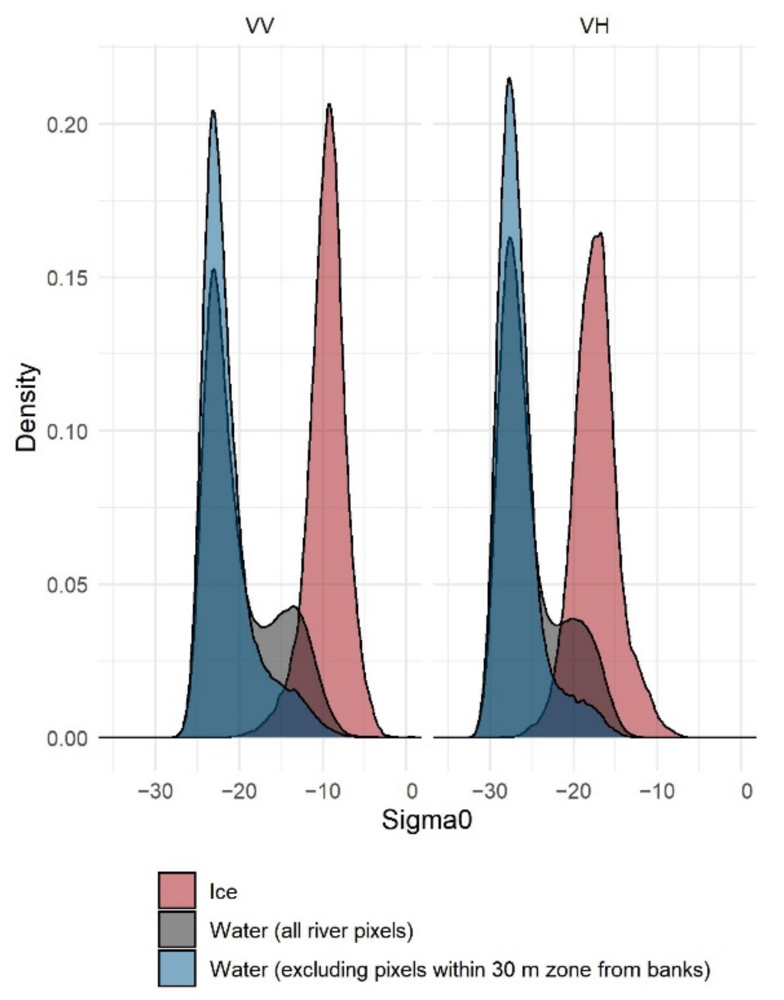
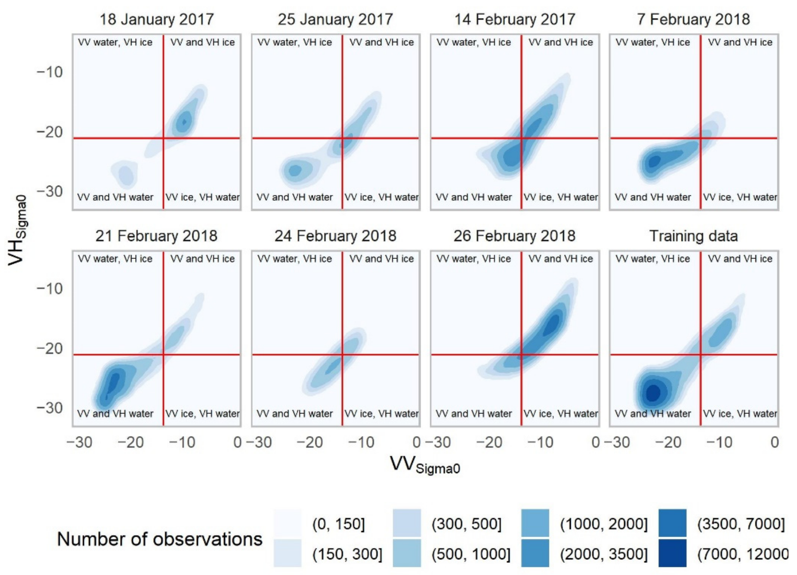
3.1. Backscatter from Ice and Open Water

To determine the optimal threshold between backscatter from water and ice, we analyzed the distribution of backscatter values from river ice and open water (Figure 2). Classification accuracy and confidence highly depends on data used to train models. During the ice season, there is a possibility that the SAR signal in individual river pixels can be reflected by both ice and open water. In extreme cases, the Nemunas and Neris River ice season starts in November and lasts until April. Thus, to estimate backscatter from open water in the analyzed rivers, we used SAR data acquired in spring (10 and 13 May 2018) and autumn (3 and 6 November 2018). The mean 30-day air temperature at the Kaunas meteorological station, which is near the center of our study area, was higher than 13 °C before image acquisition in spring and higher than 8 °C before image acquisition in autumn. The formation of ice in such conditions is highly unlikely. Thus, we are confident that the observed signal was from open water. We used the Sentinel-1 SAR data from 6 March 2018 to estimate the backscatter from river ice. We used these data because Sen2Cor scene classification showed large parts of analyzed rivers (98% of pixels) covered with ice only on that day. All Sentinel-1 pixels acquired on this day were assigned to the Sen2Cor ice class. With most of rivers’ surfaces covered with ice, there was a high confidence that the backscatter was from ice, even if ice field moved between the acquisition of Sentinel-1 and Sentinel-2 data. On other days with available Sen2Cor classes, the large river sections were covered with floating ice, which could have moved between the sensing times of both satellites, leading to a higher uncertainty in the distribution of backscatter from the ice class. We had a highly unbalanced dataset for model development, with 30,557 backscatter values of ice pixels and 207,645 values of water pixels.

Even without ice, the distribution of SAR backscatter from the pixels in the analyzed rivers was bimodal (Figure 2). Higher backscatter values were from the pixels in areas near riverbanks and were likely caused by mixed land-water pixels due to the backscatter from aquatic and riparian vegetation or exposed river bottoms. Using a trial-and-error method, we decided to use only pixels located farther than 30 m away from riverbanks, thus removing pixels that could cause uncertainty.

The difference between the backscatter from Sen2Cor water and ice class pixels was high in both VV and VH polarizations (Figure 2). In the training dataset, the 0.1 quantile of backscatter intensity from ice pixels was −12.4 dB for VV polarization and −20.6 dB for VH polarization, and the 0.9 quantile of backscatter intensity from water pixels was −16.7 dB and −23.2 for VV and VH polarizations, respectively. The difference between the medians of backscatter in ice and water pixels was 12.9 dB in the case of VV polarization and 9.7 dB in the case of VH polarization, showing that the differentiation between backscatter values was smaller in VH polarization than in VV polarization.

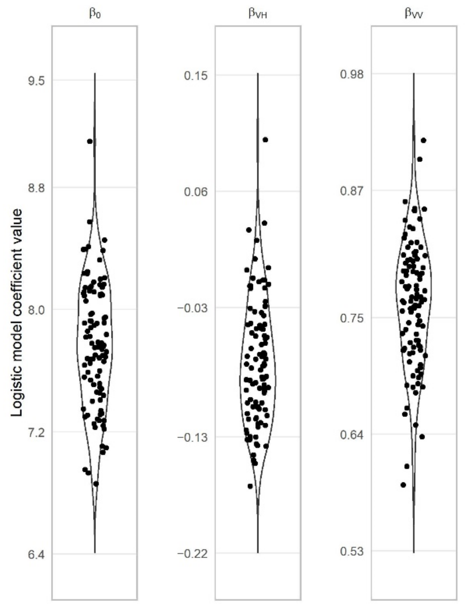
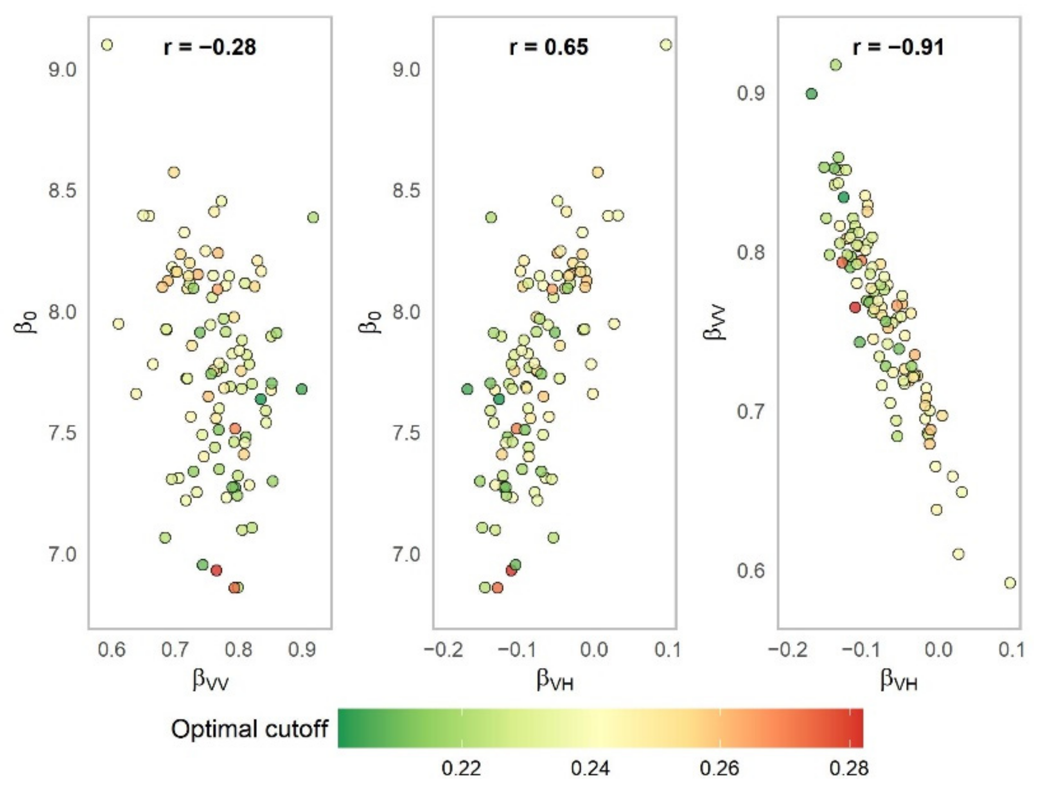
3.2. Logistic Classification Model

We fitted the logistic model to the training dataset (Table 1) using the Sen2Cor class as a target label. All model coefficients were significant (p > 0.01), but the scattering coefficient in VV polarization (β_VV = 0.76) had more than 10-times larger effect on the model result than the scattering coefficient in VH polarization (β_VH = −0.07). The correlation between the scattering coefficient in both polarizations was high (r = 0.89). Thus, the larger difference of backscatter from ice and water in VV polarization indicates that it is a more important predictor. The backscatter in VV and VH polarization had the opposite effect on the model results. The interception β₀ of the model fitted to the training dataset was 7.80.

The training dataset, considering the possible uncertainties in data and variable conditions in different parts of river, was relatively small (238,202 observations. Therefore, we used 100 subsets, selected with replacements from training dataset, to study the variability of the logistic model parameters (Figure 3). For each sample, we randomly selected 7500 observations with replacements and fitted the logistic model to them.

According to the Shapiro-Wilk test, the distributions of β₀ (p = 0.35) and β_VV (p = 0.69) were very likely to be normal, while β_VH (p = 0.04) was more likely to be deviated from normal distribution. Β_VH was negative in 94% of the cases. The variance of β_VH (mean = −0.07, standard deviation = 0.05) in comparison to the mean value was the largest of all model parameters. The value of β_VH was much smaller than β_VV, showing that its effect on the model result was less significant. The variance of β₀ (mean = 7.77, standard deviation = 0.42) and β_VV (mean = 0.76, standard deviation = 0.06) was small, indicating that the model parameters were stable with different training data. Considering that the small variation of model parameters and the mean values of the parameters of the logistic model fitted to 100 subsets were very similar to the parameters of the model fitted to the complete training dataset, we decided to use the parameters estimated with all training data for further analyses.

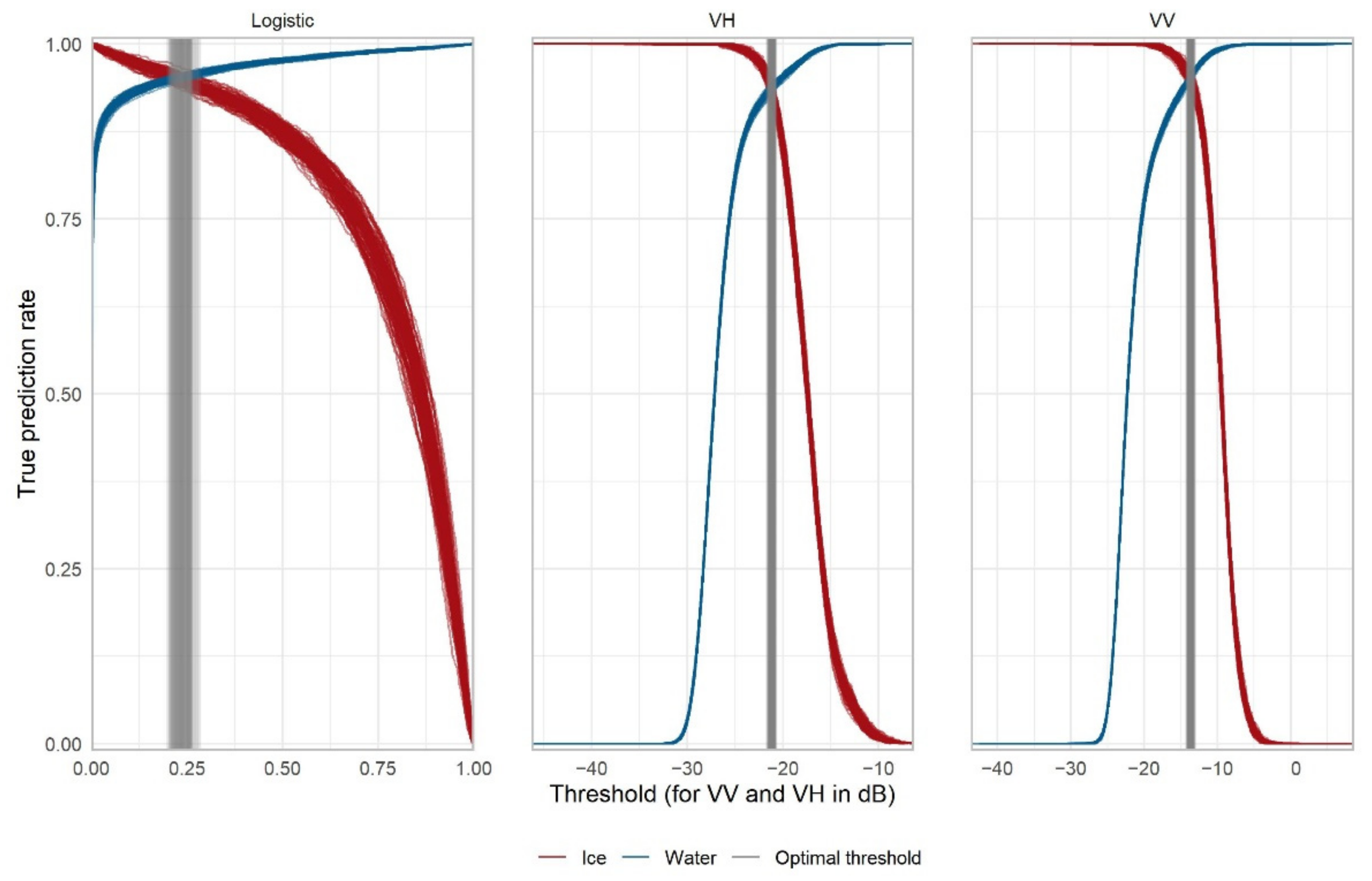
3.3. Classification Threshold

To use SAR backscatter values in binary classification, the threshold dividing the ice and water classes must be estimated. In this study, we determined the optimal threshold for the classification models based on VV and VH polarization backscatter, as well as the logistic model, using the sensitivity and specificity (true negative rate) of classification with different threshold values. The sensitivity (true positive rate) in our case corresponds to the ratio of correctly identified ice, and the specificity (true negative rate) shows correctly detected water. The aim is to develop a classification model for the correct identification of both ice and water. Thus, the optimal threshold value for a classification is where the specificity and sensitivity are equal (Figure 4). We tested the stability of all three classification models threshold value using the same 100 subsets of training data used to analyze the variability of the logistic model parameters. The sensitivity and specificity of the logistic classification model were calculated using 100 logistic models fitted to a particular subsample of data.

The variability of the optimal threshold for river surface type classification was based on the VV polarization scattering coefficient (mean = −13.7 dB, standard deviation = 0.2 dB) and VH polarization scattering coefficient (mean = −21.2 dB, standard deviation = 0.2 dB) was small (Figure 4). The variation of the optimal threshold was relatively large in the case of the logistic model (mean = 0.24, standard deviation = 0.02 dB).

The classification based on the logistic model had a larger degree of freedom than the classification based on the scattering coefficient in VV or VH polarization. The combination of the β₀, β_VV and β_VH parameters might determine the optimal threshold value for a particular logistic model. If the relationship between combinations of parameters of a particular model and its threshold value is strong, then it can be used to reduce the optimal threshold variability by interlinking the model parameters and reducing the degree of freedom.

The model parameters β_VV and β_VH were highly correlated in models fitted to 100 training data subsets (Figure 5). These parameters were linearly combined in the logistic model Equation (1), and the increase of the β_VV parameter compensated the decrease of the β_VH parameter. There was also a strong positive correlation between the β₀, and β_VH parameters (Figure 5). The optimal threshold value of the analyzed models had no clear link to the combinations of logistic model parameters. High and low threshold values were scattered in the parameter space without clear patterns (Figure 5), showing that the reduction of degrees of freedom is not likely to significantly affect the variability of optimal threshold values.

Due to uncertainties in the observation phase and the pre-processing of SAR data, the best reasonable precision for scattering coefficient in VV and VH polarizations and its threshold value used for classification is 1. Considering the variability of logistic model parameters, the threshold value with precision higher than 2 is also not likely to be practical. The variability of estimated thresholds was small in comparison to desired precision. Thus, we used the mean of estimated threshold values for river ice detection (

Table 2. River ice detection models developed using Nemunas River Sentinel-1 SAR backscatter.

Model	Equation
VV	water 0 = VVSigma0 < −13.7 dB ice = VVSigma0 ≥ −13.7 dB
VH	water = VHSigma0 < −21.2 dB ice = VHSigma0 ≥ −21.2 dB
Logistic	ice = 7.8 + 0.76 × VVSigma0 − 0.07 × VHSigma0 < 0.24 water = 7.8 + 0.76 × VVSigma0 − 0.07 × VHSigma0 ≥ 0.24

).

The classification threshold for VH was very similar to the one used in the Copernicus RLIE products (−22.3 dB). However, in our study the threshold for VV polarization was significantly higher than the one used in RLIE products (−16.7 dB) [34].

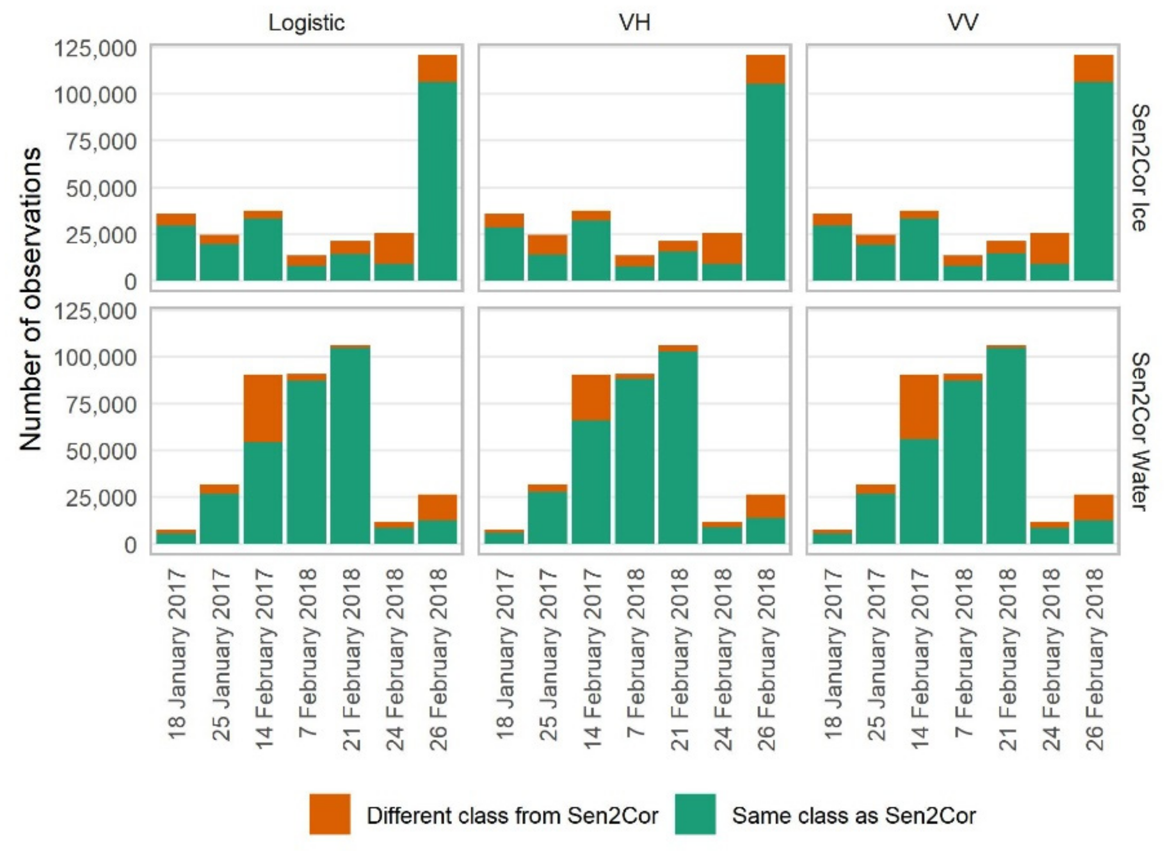
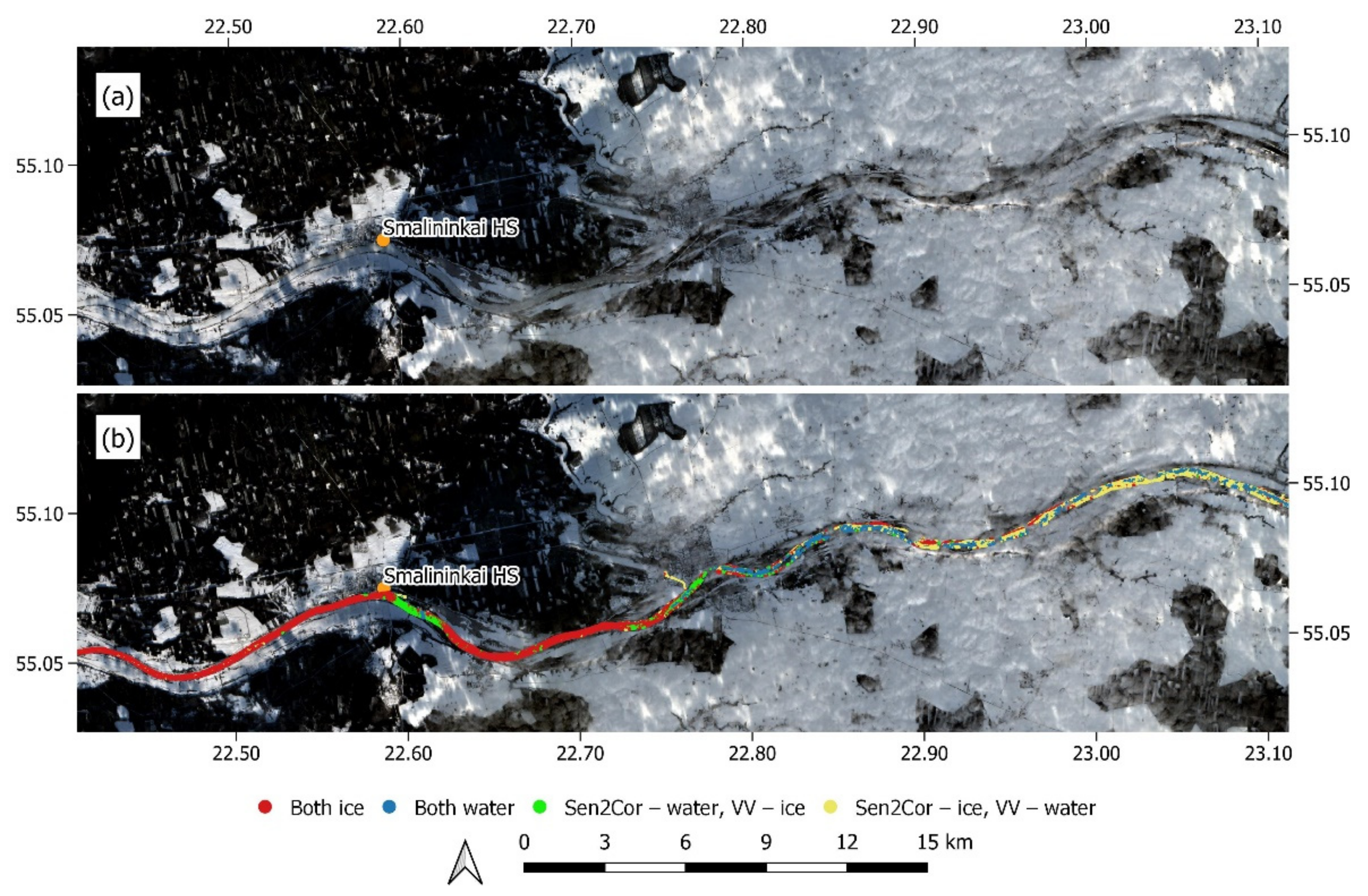
3.4. Model Validation

The goal of binary classification is to assign discrete classes to continuous data. This discrimination between ice and open water classes works best when observations are in separate clusters divided by the selected threshold. In training data, we had two clusters: one for pixels with ice and one for pixels with water (Figure 6). We had a variety of conditions in our testing dataset. Most of the pixels from 18 January 2017 and 21 February 2018 were in two distinct clusters, and only a few pixels were near the classification threshold point. Similarly, most of the pixels from 25 January 2017 were in two distinct clusters, but one of the clusters, which is likely to be composed of pixels with ice cover, was located near the crossing of classification thresholds of VH and VV polarizations (Figure 6). On other dates, the pixels did not form distinct ice and open water clusters. In the following part of results section, we examine the accuracy of binary classification under different distribution of backscatter values, compare the results of different SAR classification methods with each other and compare them to Sen2Cor classification (

Table 3. The proportion of matching logistic, VH, VV and Sen2Cor classification model classes for water and ice on different days in the testing and training datasets.

Date	VV with Sen2Cor	VH with Sen2Cor	Logistic with Sen2Cor	Logistic with VV	Logistic with VH	VH with VV
18 January 2017	80.5	79.1	80.5	99.6	93.3	93.6
25 January 2017	81.7	73.8	82.2	99.0	84.8	85.8
14 February 2017	69.9	76.7	68.4	97.8	80.8	83.1
7 February 2018	91.2	91.5	91.0	99.6	94.1	94.5
21 February 2018	93.6	93.1	93.5	99.7	96.1	96.4
24 February 2018	46.7	47.6	46.6	98.6	83.0	84.4
26 February 2018	80.9	80.4	80.8	99.4	90.0	90.6
Training data	95.2	93.7	95.4	99.7	96.7	97.0

, Figure 7).

The VV and logistic classification models performed very similarly using the training dataset and testing data. The largest difference between these models was on 14 February 2017 when the VV and logistic models predicted different classes for 2.2% of all pixels (Table 3). The mismatched cases were scattered, and their spatial distribution was sporadic. There was a larger disagreement between VV and VH classification. More than 10% of pixels were assigned to a different class on 25 January 2017, 14 February 2017 and 24 February 2018. In the following paragraphs, we present a more detailed analysis of the agreement between SAR-based classification and Sen2Cor ice and water classes. We focus on the possible causes of classification uncertainty and model performance under different ice conditions.

3.4.1. Translucent Clouds and Cloud Shadow

On 18 January 2017, we had Sentinel-1 and Sentinel-2 matchup data for a 95 km-long Nemunas River section (Figure 1). Border ice formed along banks in the eastern part of this river section, while the middle of the river channel remained open from ice. Starting from 10 km upstream from the Smalininkai HS river, the river section was covered with consolidated ice (Figure 8). Thin and translucent clouds, undetected by the Sentinel-2 cloud masking process, partly covered this river section, and contributed to the mismatch of Sen2Cor and SAR-based classification results. Visual analysis of Sentinel-2 image revealed that many pixels classified by Sen2Cor as ice were in open water, and pixels in the cloud shadow were classified as open water even if they were covered with ice. SAR-based classification methods were not affected by clouds or their shadows, and were more accurate than Sen2Cor classification in this part of the river.

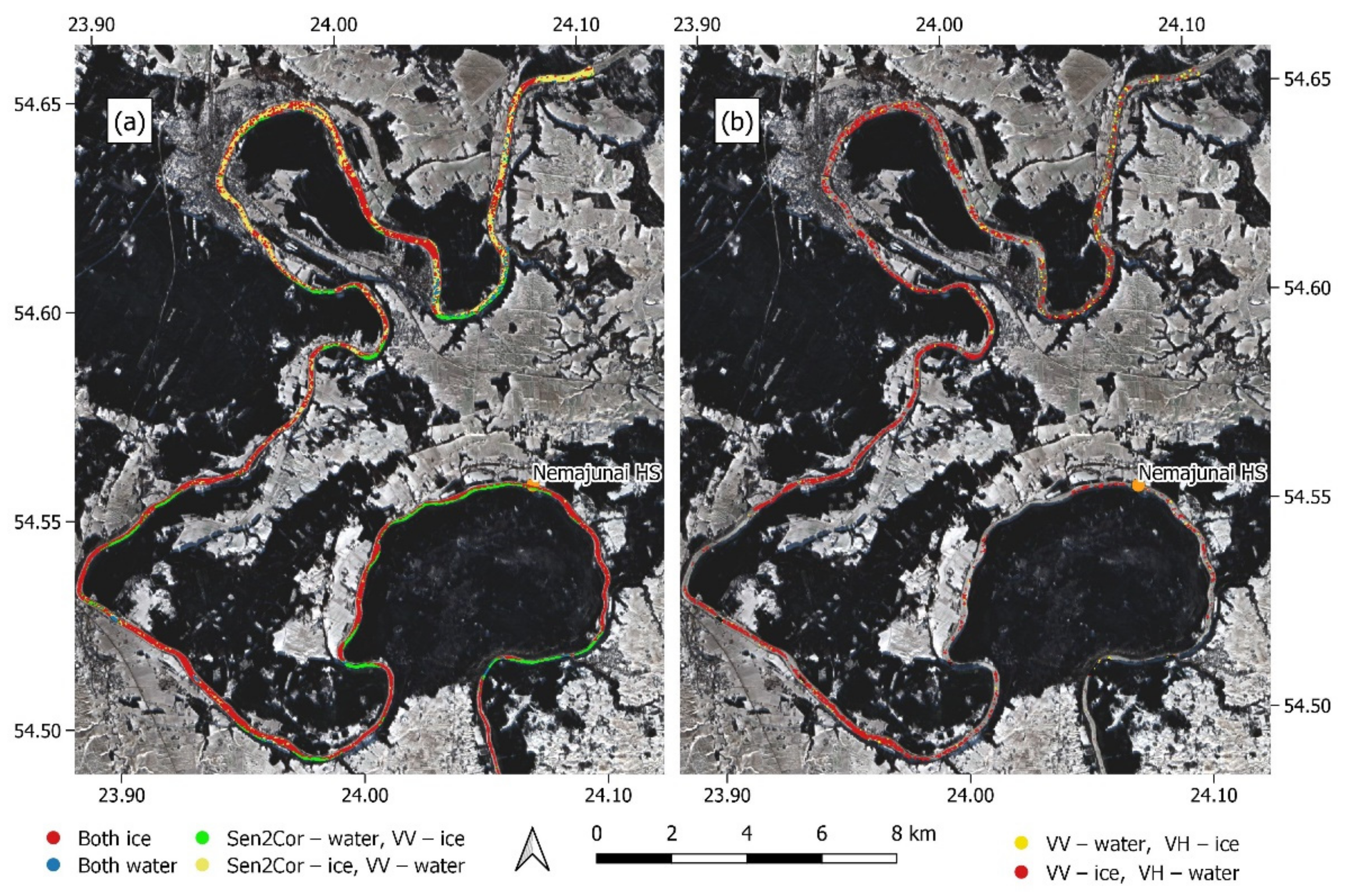
3.4.2. Effect of Reservoir and River Valley Shadows

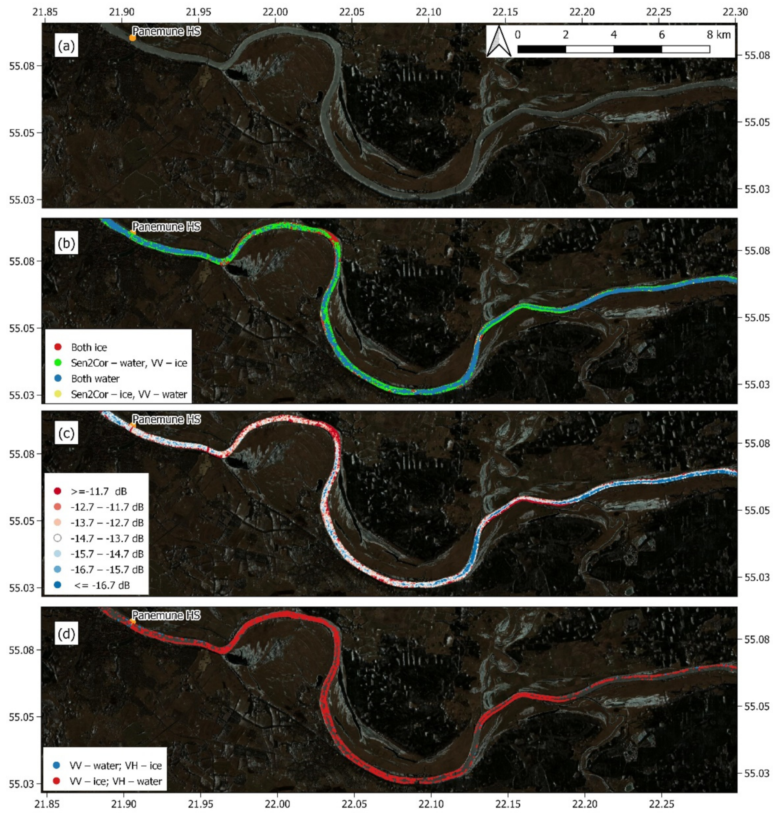
On 25 January 2017, we had overlapping Sentinel-1 and Sentinel-2 data in a large part of the Neris River and in the Nemunas River upstream from the Kaunas HPS Reservoir (Figure 1). The consolidated ice was in a 40 km section of the Neris River near the Vilnius HS, and a 130 km section of the Nemunas River upstream from the Kaunas HPS Reservoir. In other sections of the analyzed rivers, only border ice was observed. The agreement between Sen2Cor and SAR-based classification was high in the Neris River (89% with the VV and logistic model, and 86% with VH). The largest mismatch of classes was in areas with shadow cast by the steep river valley near south-eastern riverbanks. In these areas, the Sen2Cor misclassified ice cover as water.

The largest differences between Sen2Cor and SAR classification results were in the Nemunas River. Only 68% of pixels had the same VH class as the Sen2Cor class. The VV and logistic model classifications had better agreement with Sen2Cor (78% and 79%, respectively). Similar to the case of the Neris River, Sen2Cor classified pixels in the shadow of valley as water even if they were covered with ice. This effect was most noticeable in the river part near the Namajunai HS (Figure 9a), where the valley slopes are high and steep.

In the part of Nemunas River that is the closest to Kaunas HPS Reservoir (north from the Nemajunai HS), the SAR-based methods classified many pixels as water (Figure 9a), while Sen2Cor and visual inspection of the Sentinel-2 image revealed that almost all river surfaces were covered by consolidated ice or very dense frazil ice. In this part of the river, Sen2Cor classification was more accurate on 25 January 2017. It is likely that the slower current before the reservoir affected the ice formation conditions, making accumulated ice smoother and SAR backscatter lower. Using classification with the selected thresholds, the VH-based method was more sensitive to the slow current effect (Figure 9b) and was less accurate.

3.4.3. Water on Ice

The fraction of pixels in which Sen2Cor and SAR-based methods assigned same classes was the smallest on 24 February 2018 (Table 3), but the largest number of pixels with mismatched classes occurred on 14 February 2017 (Figure 7). On 14 February 2017, we overlapped satellite data acquired for the Nemunas River downstream from the Kaunas HPS Reservoir and for a 70 km long section of the Neris River upstream from its mouth (Figure 1). According to ground observations, the Nemunas River was covered with consolidated ice in all hydrological stations downstream from the Smalininkai HS (111 km from mouth). Visual analysis of Sentinel-2 images revealed that consolidated ice or dense ice rafts were in the 175 km river section from the river mouth. Sen2Cor assigned most pixels in this section of the river to the open water class (Figure 10).

A large portion of these pixels (27–40%) were assigned to the ice class by SAR-based methods (Figure 7). According to ground observations on the 14 February 2017, the river surface in the observer’s field of view was mostly covered with ice. Therefore, we cosnider SAR classification for this date as more accurate than Sen2Cor. The number of pixels classified by the VV model as water was still large, especially downstream from the Smalininkai HS (Figure 10). The backscatter from these pixels was low (VV backscatter lower than −16.7 dB) (Figure 11c). Only 1.0% of ice pixels in training dataset had lower backscatter values, suggesting that in areas not seen by hydrological station observers, the river surface was not covered with ice or, more likely, had a layer of water above the ice.

The agreement of Sen2Cor classification with VH classification was better than with VV or logistic classification (Figure 7) on 14 February 2017. Many pixels were assigned to the water class by the VH model, while these pixels were assigned to the ice class by the VV model (Figure 11d). These differences between SAR-based VV and VH model results were in the same areas where Sen2Cor predicted water.

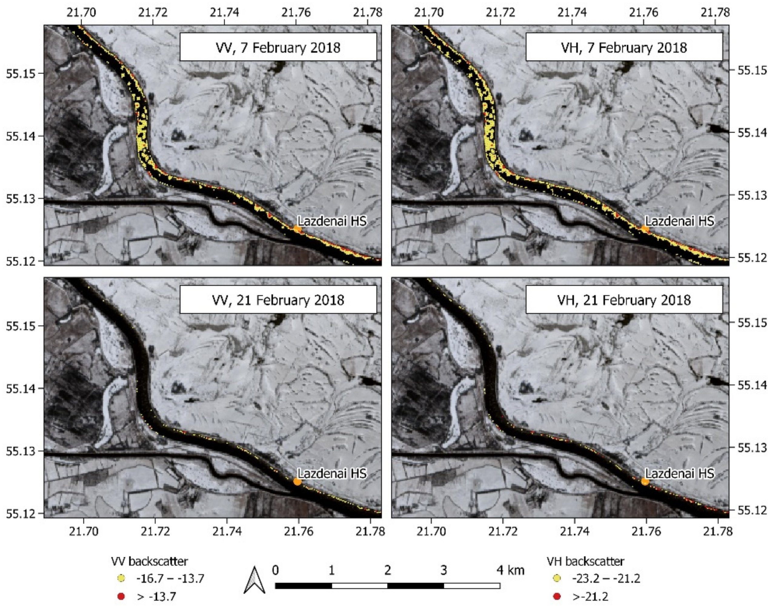
3.4.4. Frazil and Consolidated Ice

According to ground observations in 2018, ice started to form in the analyzed rivers on 6–7 February. Border ice stayed in the majority of river sections until the 26 February. At the same time, sparse and dense frazil ice appeared for short periods. The Nemunas Delta Region River was covered with consolidated ice from the 11 February until the second week of March.

On 7 February 2018, border ice and sparse frazil ice were observed in most hydrological stations. The Sen2Cor processor and SAR-based classification models detected border ice but were unable to detected frazil ice in the river channel. The largest mismatch between classes was on the edges of border ice, which was likely due to the averaging of the signal from water and ice in the pixel area, and the difference in acquisition time (7 h) between Sentinel-1 and Sentinel-2 data. The overall agreement between Sen2Cor and all SAR classification models was higher than 91% on this date, which is high considering the difference in the acquisition time of the images.

The classification would be more sensitive to sparse frazil ice if the backscatter threshold was lower. To understand if different SAR backscatter thresholds could be used to detect sparse frazil ice, we used the 0.9 quantile of backscatter values from water pixels in the training dataset (−16.7 dB for VV and −23.2 dB for VH). Using these cut-off values, an additional 13.0% (VV) and 17% (VH) of pixels would be attributed to the ice class on 7 February. A part of these pixels was adjacent to border ice, while the other part was located in the open river channel, suggesting that the pixels might represent sparse frazil ice (Figure 12). On the 21 February 2018, frazil ice was not reported, and the lowering of ice detection threshold to the 0.9 quantile of open water backscatter would lead to an increase in the ice pixels by 5.2% (VV) and 8.8% (VH). All pixels additionally classified as ice were on the edges of border ice. It seems that with the lowered threshold value, the sparse frazil ice can be detected using SAR backscatter. The trade-off of more sensitive ice detection would lead to the misclassification of water pixels. In case of this experimentation, 10% of pixels in our training dataset representing backscatter from open water in late spring and early autumn would be misclassified as ice.

On 24 February 2018, the frazil became denser. We paired satellite observations for a relatively short section of the Nemunas River between the Kaunas Lampedziai HS and Panemune HS (Figure 1). The backscatter from river pixels in most cases was close to the selected classification thresholds and formed single cluster in VV_Sigma0 and VH_Sigma0 scatterplot (Figure 6). Without a clear distinction between the backscatter from ice and water, VV and VH models both predicted that ice was in 35% of pixels with a Sen2Cor ice class, and that open water was in 72% (VV) and 75% (VH) of pixels with a Sen2Cor water class. Scattered and mostly translucent clouds in a part of Sentinel-2 image also contributed to the misclassification. For example, a 3 km river section to the west of the Smalininkai HS was covered with translucent clouds. According to Sen2Cor, the section was mostly covered with ice. However, when using VV polarization backscatter, many pixels in this part of river were classified as open water. Visual analysis of Sentinel-2 image suggests that Sen2Cor misclassified many pixels in this area, contributing to poor agreement between SAR based and Sen2Cor classification. The time gap between the Sentinel-1 and Sentinel-2 image/data acquisitions was almost 7 h and might have affected the agreement of both classification methods, especially when ice was not consolidated and its arrangement in river could quickly change. The best agreement between the VV and Sen2Cor classification methods was in areas with border ice and in areas of river channel where dense frazil ice was concentrated due to the river flow pattern. The difference between the VV and VH classification results was the largest on 24 February (15.6% of pixels). Many of the pixels classified as ice by the VV model and as water by the VH model were in areas with dense frazil ice. It is likely that VV polarization backscatter with the threshold used in our study is better is better at detecting floating river ice.

During next 2 days, the ice conditions changed. On 26 February, consolidated ice was observed in all hydrological stations downstream from the Kaunas Lampedziai HS. In this part of the river, the concurrence between Sen2Cor and SAR-based classifications was high despite the large difference in the acquisition time of the Sentinel-1 (26 February 2018 16:03) and Sentinel-2 (27 February 2018 09:50). The differences between classification results mostly occurred in the Neris River and Nemunas River upstream from the Kaunas Reservoir. In both sections with the lowest classification correlation, observers recorded frazil ice.

4. Discussion

In situ observations have some degree of uncertainty. An observer uses standard ice type classes to describe ice conditions in his field of view. The detected ice class depends on the experience of the observer and his interpretation, and might also depend on the visibility. Despite these facts, ground observations are the most reliable source of information about river ice conditions.

Optical satellite data with a high resolution and large spatial extent provides a prospective alternative to ground observations of ice in the development of machine learning ice classification algorithms. The development procedure of machine learning algorithms involves the use of large quantities of data. Our study results suggest that the additional manual assessment of the quality of optical images is necessary before they can be used as data representing ground truth in the development of SAR-based river ice detection models. After the visual analysis of Sentinel-2 images, we found many cases when the river pixels were classified as ice with Sen2Cor due to scattered and often translucent cloud cover. These clouds were not detected by scene classification algorithms and were not included in the cloud mask. Cloud and river valley shadows also contributed to the misclassification of ice pixels.

Even in cases of mismatch between Sen2Cor classes and predictions of SAR-based classification models, the SAR models agreed better with the ground observations and manual Sentinel-2 image interpretation results. SAR-based models were unable accurately represent river ice conditions only in the Nemunas section with hydrology and ice formation affected by the Kaunas HPS Reservoir. This fact highlights the importance of local studies, because even models developed using data from the same river might not be accurate in sections with diverse conditions. We used 100 subsets in the training dataset to test the stability of the classification model thresholds. The variation of optimal threshold values was relatively small, even though our training dataset represented a river section with uniform hydrological and morphological conditions. Selected thresholds performed well in all analyzed Nemunas River and Neris River parts except the section near the Kaunas HPS Reservoir. It is likely that most optimal solution for this part of the river would be to develop dedicated ice detection models. There were no rapids or locations with significantly rough water surfaces in the analyzed river sections. Thus, we could not estimate how rough water might affect the ice detection accuracy with models used in this study. Other studies have encountered difficulties detecting river ice with SAR-based methods near rapids [13].

The Sentinel-1 acquisition time was ≈5 h earlier or ≈7 h later than the acquisition time of Sentinel-2 in the study area (Table 1). SAR-based ice classification models agreed better with the Sen2Cor class when river ice was consolidated and not moving. This is likely related to the different backscatter properties of moving and consolidated ice.

The difference of backscatter from open water and ice in the analyzed rivers was significant, but the backscatter from river pixels was in clearly separate clusters representing water and ice only in several cases. Frequent mild winters lead to very variable ice conditions in the rivers. In most cases, cold spells are short, and only border and frazil ice form. All SAR and Sen2Cor classification models performed better detecting consolidated, border and dense frazil ice than sparse frazil ice. The analysis of SAR backscatter from river surfaces with and without frazil ice suggests that even sparse frazil ice can increase backscatter from the river surface. However, without visual data collected on the ground, it is impossible to quantify how different types of frazil ice can affect the backscatter. The information on hydrological and meteorological conditions is also necessary to increase confidence of these results. For long river sections with uniform ice properties, the radar incidence angle [21,35] might be an important factor affecting backscatter intensity and ice detection confidence. We did not find a clear effect of the incidence angle on the backscatter from ice and water on the analyzed days, most likely because it was outweighed by the high spatial variability of ice types and ice properties.

In this analysis, we optimized classification models to provide the most accurate classification for both ice and water classes. We selected the classification threshold at the point where the sensitivity was equal to specificity. If the goal is to identify the beginning of the ice season or detect sparse frazil ice, then a different approach could be used. For example, using a similar classification threshold for VV backscatter (−16.9 dB) as in the Copernicus River and Lake Ice Extent products [34], we were more likely to detect frazil ice on 7 February 2018. At the same time, the risk of classifying water pixels as ice would be much higher. Using this threshold, about 10% of the pixels in our model training data, acquired during warm weather conditions in May and November (Table 1), would be assigned to the ice class.

VV backscatter- and logistic model-based classification gave very similar results. The VV and logistic model classification result was the same in 99.3% of all cases in the testing dataset. This fact is not surprising because VV_Sigma0 had a much larger weight in the logistic model equation than VH_Sigma0. The application of VV-based classification is more practical for ice detection than logistic model classification. With VV classification, the same result can be achieved using one polarization data instead of two. In addition, the application of logistic model is an additional step, which can be avoided to save time and resources. The most important advantage of the VV polarization-based classification is that its results are easier to interpret than the logistic model output, which is useful in the assessment of classification accuracy, and might increase user confidence and uptake.

The classification using VV polarization agreed better with Sen2Cor than VH classification on all analyzed dates except 14 February 2017. On this date, VH polarization-based classification had better agreement with Sen2Cor, but at the same time, according to ground observations, Sen2Cor misclassified many ice pixels as water. Having that in mind, it is likely that the VV classification model performed better than the VH model, even on 14 February 2017.

As mentioned before, all SAR-based classification methods misclassified large fraction of pixels with ice upstream from the Kaunas HPS Reservoir, but VH polarization backscatter was more affected than VV backscatter. In the large proportion of pixels in this part of the river, VH backscatter was lower than the classification threshold, while VV backscatter was higher than the threshold (Figure 9), correctly predicting ice. VH classification was also not as accurate as VV classification in the case of floating river ice.

These facts suggest that, at least in the analyzed sections of the Nemunas and Neris rivers, ice detection using VV polarization backscatter would be more accurate than using VH backscatter and more feasible than using the logistic model.

In this study, we evaluated model accuracy on a pixel basis, but such approach is not necessary in the practical application of ice extent detection models. It is more important to detect river sections with ice than to be confident in the class of the individual pixel. Thus, spatial reducers, such as the majority, would be likely applied in practice. The accuracy of individual pixel classification remains important because it affects the confidence of the aggregation result.

5. Conclusions

The river ice detection based on optical data had large uncertainties related to cloud cover and shadows. Thus, it cannot be reliably used as a single ground truth source in the quantitative evaluation of SAR-based ice detection model accuracy. Additional ground observation data and the manual interpretation of optical images are necessary to understand the prediction accuracy. Sentinel-1 SAR models were more reliable and more accurate in Nemunas and Neris River ice detection than Sentinel-2 MSI Sen2Cor scene classification. The ice detection model based on VV polarization backscatter performed better than the model based on VH backscatter. The correlation between the predictions of the VV model and logistic model, linearly combining VV and VH polarization backscatter, was r = 0.99. Thus, the use of logistic model does not offer significant gains in practice.

The optimal thresholds of the classification model-estimated findings when specificity was equal to sensitivity performed well in most parts of the Neris and Nemunas Rivers, except the section in which river hydrology was affected by the Kaunas HPS Reservoir. To achieve better classification accuracy, separate ice detection models could be developed for river sections with diverse hydrology and morphology. With the determined thresholds, we were able to detect consolidated, border and dense frazil ice. However, in the case of sparse frazil ice, the detection threshold had to be lowered, increasing model sensitivity.

Our study results support that Sentinel-1 SAR backscatter can be used to detect ice with high confidence, but, in most cases, the development and validation of models requires the manual inspection of training data quality and validation on river sections with different hydrological conditions. The proposed methodology would provide most confident results in lowland rivers with steady currents, but it might not be applicable in sections with disturbed water surfaces near riffles or rapids and in sections with a very slow current, for example, valley-dammed reservoirs.

References

1. Newton, A.M.W.; Mullan, D.J. Climate change and Northern Hemisphere lake and river ice phenology from 1931–2005. Cryosphere 2021, 15, 2211–2234. [Google Scholar] [CrossRef]
2. Yang, X.; Pavelsky, T.M.; Allen, G.H. The past and future of global river ice. Nature 2020, 577, 69–73. [Google Scholar] [CrossRef] [PubMed]
3. Stonevicius, E.; Stankunavicius, G.; Kilkus, K. Ice regime dynamics in the Nemunas River, Lithuania. Clim. Res. 2008, 36, 17–28. [Google Scholar] [CrossRef] [Green Version]
4. Knoll, L.B.; Sharma, S.; Denfeld, B.A.; Flaim, G.; Hori, Y.; Magnuson, J.J.; Straile, D.; Weyhenmeyer, G.A. Consequences of lake and river ice loss on cultural ecosystem services. Limnol. Oceanogr. Lett. 2019, 4, 119–131. [Google Scholar] [CrossRef] [Green Version]
5. Gauthier, Y.; Weber, F.; Savary, S.; Jasek, M. A combined classification scheme to characterise. EARSeL Eproc. 2006, 5, 77–88. [Google Scholar]
6. Duguay, C.R.; Bernier, M.; Gauthier, Y.; Kouraev, A. Remote Sensing of Lake and River Ice; Wiley: Hoboken, NJ, USA, 2014; ISBN 9781118368909. [Google Scholar]
7. Turcotte, B.; Morse, B. A global river ice classification model. J. Hydrol. 2013, 507, 134–148. [Google Scholar] [CrossRef]
8. Łoś, H.; Osińska-Skotak, K.; Pluto-Kossakowska, J.; Bernier, M.; Gauthier, Y.; Pawłowski, B. Performance evaluation of quad-pol data compare to dual-pol SAR data for river ice classification. Eur. J. Remote Sens. 2019, 52, 79–95. [Google Scholar] [CrossRef] [Green Version]
9. Chu, T.; Das, A.; Lindenschmidt, K.E. Monitoring the variation in ice-cover characteristics of the Slave River, Canada using RADARSAT-2 Data-A case study. Remote Sens. 2015, 7, 13664–13691. [Google Scholar] [CrossRef] [Green Version]
10. Gauthier, Y.; Tremblay, M.; Bernier, M.; Furgal, C. Adaptation of a radar-based river ice mapping technology to the Nunavik context. Can. J. Remote Sens. 2010, 36, S168–S185. [Google Scholar] [CrossRef]
11. Lindenschmidt, K.E. Characterising river ice along the Lower Red River using RADARSAT-2 imagery. In Proceedings of the 16th Workshop on River Ice, Winnipeg, MB, Canada, 8–11 September 2011; pp. 1–16. [Google Scholar]
12. Surdu, C.M.; Duguay, C.R.; Pour, H.K.; Brown, L.C. Ice freeze-up and break-up detection of shallow lakes in Northern Alaska with spaceborne SAR. Remote Sens. 2015, 7, 6133–6159. [Google Scholar] [CrossRef] [Green Version]
13. Jasek, M.; Gauthier, Y.; Poulin, J.; Bernier, M. Monitoring of freeze-up on the Peace River at the Vermilion Rapids using RADARSAT-2 SAR data. In Proceedings of the 17th Workshop on River Ice, Edmonton, AB, Canada, 21–24 July 2013; pp. 229–257. [Google Scholar]
14. Gherboudj, I.; Bernier, M.; Leconte, R. A backscatter modeling for river ice: Analysis and numerical results. IEEE Trans. Geosci. Remote Sens. 2010, 48, 1788–1798. [Google Scholar] [CrossRef]
15. Mermoz, S.; Allain-Bailhache, S.; Bernier, M.; Pottier, E.; Van Der Sanden, J.J.; Chokmani, K. Retrieval of river ice thickness from C-band PolSAR data. IEEE Trans. Geosci. Remote Sens. 2014, 52, 3052–3062. [Google Scholar] [CrossRef] [Green Version]
16. Los, H.; Pawlowski, B. The use of Sentinel-1 imagery in the analysis of river ice phenomena on the lower Vistula in the 2015–2016 winter season. In Proceedings of the 2017 Signal Processing Symposium (SPSympo), Debe, Poland, 12–14 September 2017; p. 4. [Google Scholar] [CrossRef]
17. Drouin, H.; Gauthier, Y.; Bernier, M.; Jasek, M.; Penner, O.; Weber, F. Quantitative validation of RADARSAT-1 river ice maps. In Proceedings of the 14th Workshop of the Committee on River Ice Processes and the Environment, Quebec City, QC, Canada, 19–22 June 2007; p. 18. [Google Scholar]
18. Nagler, T.; Rott, H.; Ripper, E.; Bippus, G.; Hetzenecker, M. Advancements for snowmelt monitoring by means of Sentinel-1 SAR. Remote Sens. 2016, 8, 348. [Google Scholar] [CrossRef] [Green Version]
19. Zubaničs, A. River ice detection on The Daugava River using Sentinel-1 SAR data. In Proceedings of the 100th AMS Annual Meeting, Boston, MA, USA, 12–16 January 2019; p. 1. [Google Scholar]
20. Pantea, G.; Lacusteanu, A. Monitoring of the freezing Danube delta based on Sentinel-1/2 imagery. J. Young Sci. 2017, 5, 213–218. [Google Scholar]
21. De Roda Husman, S.; van der Sanden, J.J.; Lhermitte, S.; Eleveld, M.A. Integrating intensity and context for improved supervised river ice classification from dual-pol Sentinel-1 SAR data. Int. J. Appl. Earth Obs. Geoinf. 2021, 101, 102359. [Google Scholar] [CrossRef]
22. Ning, L.; Xie, F.; Gu, W.; Xu, Y.; Huang, S.; Yuan, S.; Cui, W.; Levy, J. Using remote sensing to estimate sea ice thickness in the Bohai Sea, China based on ice type. Int. J. Remote Sens. 2009, 30, 4539–4552. [Google Scholar] [CrossRef]
23. Tom, M.; Prabha, R.; Wu, T.; Baltsavias, E.; Leal-Taixé, L.; Schindler, K. Ice monitoring in Swiss lakes from optical satellites and webcams using machine learning. Remote Sens. 2020, 12, 3555. [Google Scholar] [CrossRef]
24. Kraatz, S.; Khanbilvardi, R.; Romanov, P. River ice monitoring with MODIS: Application over Lower Susquehanna River. Cold Reg. Sci. Technol. 2016, 131, 116–128. [Google Scholar] [CrossRef]
25. Chaouch, N.; Temimi, M.; Romanov, P.; Cabrera, R.; Mckillop, G.; Khanbilvardi, R. An automated algorithm for river ice monitoring over the Susquehanna River using the MODIS data. Hydrol. Process. 2014, 28, 62–73. [Google Scholar] [CrossRef]
26. Beaton, A.; Whaley, R.; Corston, K.; Kenny, F. Identifying historic river ice breakup timing using MODIS and Google Earth Engine in support of operational flood monitoring in Northern Ontario. Remote Sens. Environ. 2019, 224, 352–364. [Google Scholar] [CrossRef]
27. Li, H.; Li, H.; Wang, J.; Hao, X. Monitoring high-altitude river ice distribution at the basin scale in the northeastern Tibetan Plateau from a Landsat time-series spanning 1999–2018. Remote Sens. Environ. 2020, 247, 111915. [Google Scholar] [CrossRef]
28. Selkowitz, D.J.; Forster, R.R. An automated approach for mapping persistent ice and snow cover over high latitude regions. Remote Sens. 2016, 8, 16. [Google Scholar] [CrossRef] [Green Version]
29. Prabha, R.; Tom, M.; Rothermel, M.; Baltsavias, E.; Leal-Taixe, L.; Schindler, K. Lake ice monitoring with webcams and crowd-sourced images. arXiv 2020, arXiv:2002.07875. [Google Scholar] [CrossRef]
30. HR-S&I Consortium. Pan-European High-Resolution Snow & Ice Monitoring of the Copernicus Land Monitoring Service—Production of Basic Products Quality Assessment Report for Ice Products Based on Sentinel-2. 2021. Available online: https://land.copernicus.eu/user-corner/technical-library/hrsi-ice-atbd (accessed on 24 March 2022).
31. Lindenschmidt, K.-E.; Li, Z. Monitoring river ice cover development using the Freeman–Durden decomposition of quad-pol Radarsat-2 images. J. Appl. Remote Sens. 2018, 12, 026014. [Google Scholar] [CrossRef]
32. SNAP. Available online: https://step.esa.int/main/toolboxes/snap/ (accessed on 24 March 2022).
33. Main-Knorn, M.; Pflug, B.; Louis, J.; Debaecker, V.; Müller-Wilm, U.; Gascon, F. Sen2Cor for Sentinel-2. In Proceedings of the SPIE 2017, 10427, Image and Signal Processing for Remote Sensing XXIII, Bellingham, DC, USA, 11–13 September 2018. [Google Scholar] [CrossRef] [Green Version]
34. HR-S&I Consortium. Pan-European High-Resolution Snow & Ice Monitoring Of The Copernicus Land Monitoring Service Algorithm Theoretical Basis Document For Ice Products Based On Sentinel-1 & Sentinel-2. 2021. Available online: https://land.copernicus.eu/user-corner/technical-library/hrsi-ice-s1-atbd/ (accessed on 24 March 2022).
35. DeLancey, E.R.; Kariyeva, J.; Cranston, J.; Brisco, B. Monitoring hydro temporal variability in Alberta, Canada with multi-temporal sentinel-1 SAR data. Can. J. Remote Sens. 2018, 44, 1–10. [Google Scholar] [CrossRef]
Figure 1. The Lithuanian part of the Nemunas and Neris Rivers, the location of hydrological stations (black dots) with available ground observation data and river sections (color stripes) covered by the matching Sentinel-1 SAR and Sentinel-2 MSI observations used for the development and validation of the river ice detection models.
Remotesensing 14 01627 g001
Figure 2. The distribution of backscatter coefficient Sigma0 from ice (6 March 2018) and open water pixels (data from 10 and 13 May, 3 and 6 November 2018), including and excluding the zone within 30 m away from riverbanks.
Remotesensing 14 01627 g002
Figure 3. The distribution of logistic model coefficients estimated using 100 training dataset subsets, each consisting of 7500 pixels. Points were randomly jittered in horizontal direction to avoid overlapping.
Remotesensing 14 01627 g003
Figure 4. Optimal ice and open water classification thresholds of the logistic, VH and VV models determined using 100 training dataset subsets. The threshold was considered optimal, and the true prediction rates for water (specificity) and ice (sensitivity) were equal.
Remotesensing 14 01627 g004
Figure 5. Interdependency between logistic model parameters β0, βVV, βVH and ice/water classification threshold value estimated using 100 training dataset subsets.
Remotesensing 14 01627 g005
Figure 6. Distribution of observations in the VVSigma0 and VHSigma0 plain on different dates in the testing and training datasets. Red lines represent the ice and water classification thresholds used in models based on VV and VH polarization backscatter.
Remotesensing 14 01627 g006
Figure 7. The agreement of SAR-based logistic, VH and VV model classification with the Sen2Cor ice and water classes on different days from the testing dataset.
Remotesensing 14 01627 g007
Figure 8. Nemunas River section near the Smalininkai HS affected by the translucent clouds and their shadows on 18 January 2017. The effect of clouds and their shadows for ice detection is visible in Sentinel-2 natural color composite (a) and the match of Sen2Cor classes with the VV model prediction (b).
Remotesensing 14 01627 g008
Figure 9. Nemunas River section between the Nemajunai HS and Kaunas HPS Reservoir (north from shown section) on 25 January 2017 was covered by ice. Sen2Cor predicted water class in the river valley shadow, while the VH model misclassified many pixels as water upstream from the HPS Reservoir (a). The VH model classified more pixels as water than the VV model (b).
Remotesensing 14 01627 g009
Figure 10. VV model prediction compared to the Sen2Cor class on 14 February 2017.
Remotesensing 14 01627 g010
Figure 11. Sentinel-2 natural color composition (a), VV model prediction compared to Sen2Cor class (b), VV polarization backscatter coefficient (c) and VV and VH classification mismatch (d) on 14 February 2017 in the Nemunas River upstream from the Panemunes HS.
Remotesensing 14 01627 g011
Figure 12. Sentinel-1 SAR backscatter in VV and VH polarizations in Nemunas River near the Lazdenai HS on a day with sparse frazil ice (7 February 2018) and without frazil ice (21 February 2018).
Remotesensing 14 01627 g012