An Accuracy Assessment of Snow Depth Measurements in Agro-Forested Environments by UAV Lidar

Abstract

This study assesses the performance of UAV lidar system in measuring high-resolution snow depths in agro-forested landscapes in southern Québec, Canada. We used manmade, mobile ground control points in summer and winter surveys to assess the absolute vertical accuracy of the point cloud. Relative accuracy was determined by a repeat flight over one survey block. Estimated absolute and relative errors were within the expected accuracy of the lidar (~5 and ~7 cm, respectively). The validation of lidar-derived snow depths with ground-based measurements showed a good agreement, however with higher uncertainties observed in forested areas compared with open areas. A strip alignment procedure was used to attempt the correction of misalignment between overlapping flight strips. However, the significant improvement of inter-strip relative accuracy brought by this technique was at the cost of the absolute accuracy of the entire point cloud. This phenomenon was further confirmed by the degraded performance of the strip-aligned snow depths compared with ground-based measurements. This study shows that boresight calibrated point clouds without strip alignment are deemed to be adequate to provide centimeter-level accurate snow depth maps with UAV lidar. Moreover, this study provides some of the earliest snow depth mapping results in agro-forested landscapes based on UAV lidar.

1. Introduction

One of the key features of snow accumulation is the spatial variability of the snow cover. At a broader scale, quantifying the spatial distribution of snow depth is vital to address the current behavior and the future of the cryosphere [1]. At the watershed or smaller scales, accounting for the spatial variability of snow depth is crucial to estimate the amount and timing of spring runoff [2]. Rapid changes in the amount, extent, timing, and duration of the snow cover in cold regions with changing climatic conditions—mainly in response to warming temperatures and rain-on-snow events [3,4]—call for a better knowledge of the quantification of snow distribution [5].

Given the importance of accounting for the spatial variability of the snow cover, the most frequently utilized techniques to observe snowpack variations are in situ observations and/or remote sensing. The traditional, ground-based, and mostly manual process of monitoring snow characteristics is expensive, extremely labor-intensive, time-consuming, and potentially dangerous. Additionally, it can disturb the snowpack and influence subsequent measurements [6]. Even when available, and despite its accuracy, point measurements may not be representative of a larger area [7]. Nevertheless, during the past several decades, remote sensing techniques that surmounted most of the aforementioned drawbacks have become a powerful and efficient approach for monitoring snowpack in remote environments. A variety of airborne and terrestrial remote sensing techniques developed using satellite, radar, laser (lidar: Light detection and ranging), and photogrammetry data have been extensively used in a variety of cryospheric studies [7,8]. Among these techniques, airborne (manned and unmanned) laser scanning has become increasingly popular due to its ability to capture high-resolution micro (<100 m) and mesoscale (100 m–10 km) variability, as well as to detect snow cover/ground under canopy due to its strong penetration ability [6,9,10,11,12,13,14,15,16,17,18]. In recent years, there has been a growing interest in the use of unmanned aerial vehicle (UAV) laser scanning for small scale high-resolution mapping, due to its potential to deliver dense and high-quality point clouds with minimal occlusion in forested areas compared with airborne laser scanning (ALS) [14,15,16,19,20,21,22,23]. Snow depths from lidar data are commonly estimated by differencing snow-covered and snow-free elevation products [6,9,10,24,25,26,27]. Usually, ground-based manual measurements are used as ground truth data to validate the lidar-derived snow depth products [6,7]. However, as with any other measuring technique, UAV laser scanning is not exempt from errors.

In general, the UAV lidar system comprises three instruments: A laser device, an inertial measurement unit (IMU) that continuously records platform orientation, and high precision airborne global positioning system (GNSS, global navigation satellite system), which records the three-dimensional position of the platform [6,28]. Moreover, the system requires a GNSS base station installed at a known location and in the vicinity of the airborne platform (preferably within 50 km), which operates simultaneously to differentially correct, and thus improve the precision of the airborne GNSS data [29]. Error sources of UAV lidar mapping can broadly be classified into boresight errors, navigational errors, terrain-induced errors, vegetation-induced errors, and post-processing errors [6,30]. Boresight errors occur due to offset and angular differences between the lidar and IMU origins. The origin difference vector is called boresight shift or lever-arm offset, and the three angles between the lidar and IMU axes are called boresight angles [30,31]. UAV lidar systems are more prone to boresight angular errors, due to their lower sensor installation precision and stability than lidars used onboard manned aircrafts [28,32]. Precise calibration of lever-arm offsets and boresight angles can reduce the boresight errors [28,33]. While lever-arm offsets can usually be accurately measured after system assembling or from drawings [28], boresight angle errors should be calibrated manually [31] or using automated methods [28,32,33,34].

Errors associated with GNSS and IMU can result in navigational errors. These navigational errors can be minimized with IMU calibration, as well as GNSS accuracy enhancements methods, such as differential global positioning system (DGPS), real-time kinematic (RTK), precise point positioning (PPP) or post-processing kinematic (PPK) [6]. Another method to reduce random errors caused by GNSS and IMU is the strip adjustment, which fundamentally decreases the discrepancies between flight strips. The strip adjustment (or strip alignment) technique has proven to be very successful with ALS data [35,36], and implementing it on UAV data remains an active area of research [21,37]. One of the reasons that this technique is not (yet) very popular among UAV users is that the readily available strip adjustment algorithms require raw data of the laser scanner, which is often not accessible for most end-users through the UAV lidar system [21,32].

Terrain-induced errors are mostly positional errors that occur due to complex terrain and steep terrain slopes. Flight planning can help in reducing these terrain-induced errors to some extent by minimizing oblique incident laser shots on steep slopes [6]. The presence of canopy and/or sub-canopy can reduce the number of laser shots reaching the ground or snowpack surface, and thus result in observation gaps. The density of ground return lidar points depends on the canopy type and architecture, laser spot size, laser pulse rate, scan angle, flying height, and flying speed, i.e., higher pulse rates provide more laser shots, while smaller scan angles and a lower flight altitude increase the probability of canopy penetration [6,38,39]. Therefore, a proper flight planning can minimize errors to some degree. Post-processing errors are predominantly caused by misclassification of the raw point cloud (misclassifying the terrain points as non-terrain and/or vice versa). Point cloud classification algorithms are often highly automated. As a result, the magnitude of error depends on the type of filter used, local terrain geometry, the height and type of vegetation, the presence of manmade structures, such as buildings, and the accuracy of the measured elevation [6,40,41].

Moreover, there is a lack of studies evaluating the accuracy of UAV lidar point data and lidar-derived snow depth maps with and without different vegetation covers. To our knowledge, two studies estimated the UAV-based lidar snow depth measurement accuracy to date [16,17]. Harder et al. [16] compared snow depth estimates between UAV lidar versus structure-from-motion (SfM) technique using manual snow depth measurements in mountain and prairie environments in western Canada. Jacobs et al. [17] explored the capability of UAV lidar to estimate shallow snow depths in mixed-hardwood-forest and open-field land covers in the eastern USA through the comparison of simultaneous field-based snow depth measurements. Both studies showcased the ability of UAV lidar to effectively quantify the small scale snow depth variability.

The overall motivation for this work is to understand and assess the performance of UAV lidar system in measuring high-resolution snow depths in agro-forested landscapes. Moreover, to our knowledge, this study is the first of its kind that utilized the UAV laser scanning technique to measure small scale snow depth variability in southern Québec, Canada, which houses distinct land use patterns of alternating agricultural fields and forest patches. These mosaics of forests and agricultural fields are referred to as agro-forested landscapes in southern Québec [42,43]. In addition to boresight calibration, a strip alignment method was applied to the data to test whether it can improve the accuracy of data by partly correcting high-frequency IMU errors (random errors). First, this paper discusses the data collection and processing workflow, including the sources of errors and the refinement methods implemented in this study. Then, an assessment of the absolute and relative accuracy of the lidar data, an evaluation of the accuracy of snow depth maps with manual measurements in the open field versus forested environments, and an investigation of the applicability of strip alignment with UAV lidar data are presented.

2. Materials and Methods

2.1. Study Sites

Three sites that represent the main land use and cover patterns in southern Québec were selected to test the ability of UAV lidar to measure snow depths in open and vegetated areas (Figure 1). Sainte-Marthe (45.4° N, 74.2° W) is a paired agricultural and dense deciduous forested site [44], where the forested area comprises sugar maple (Acer saccharum), red maple (Acer rubrum) with no or sparse understory, and a small conifer plantation to the Southwest. Saint-Maurice (46.4° N, 72.5° W) is a paired agricultural and high to moderate dense mixed forested site, and the forested area comprises poplar (Populus x canadensis), red maple (Acer rubrum), white pine (Pinus strobus), and balsam fir (Abies balsamea) with sparse understory. The forested areas in these sites overlie undulating glacial till sediments that are often associated with rougher microtopography, whereas the agricultural fields are associated with flatter glaciomarine or fluvioglacial sediments (Québec Ministry of Forests, Wildlife, and Parks (MFFP), Québec Research and Development Institute for the Agri-Environment (IRDA), and La Financière Agricole du Québec (FADQ)). The main crop type in the agricultural areas of these two agro-forested sites is soya. Irrigation canals and streams that flow through these open agricultural areas form distinct terrain characteristics in the exposed agricultural fields. Forêt Montmorency (hereafter Montmorency; 47.3° N, 71.1° W) is a site with dense boreal forest interspersed with large gaps. The dominant tree types in this site are balsam fir (Abies balsamea), black spruce (Picea mariana), and white spruce (Picea glauca) with no understory. Adjacent to the forest is an open area hosting the NEIGE-FM snow research station, which hosts a variety of precipitation gauges and snowpack measuring sensors, and is part of the World Meteorological Organization’s (WMO) Global Cryosphere Watch (GCW) surface network [45]. Montmorency has a combination of glacial till and fluvioglacial soil types.

Table 1. Site characteristics and field campaign details.

	Sainte-Marthe	Saint-Maurice	Montmorency
Elevation range, m	70–78	46–50	670–700
MAAT, °C	6.0	4.7	0.5
Total precipitation, mm	1000	1063	1600
Snowfall/Total Precipitation, %	15	16	40
Winter season	November–March	November–March	October–April
Lidar extent, km2	0.22	0.25	0.12
Snow-off flight date	11 May 2020	02 May 2020	13 June 2019
Snow-on flight date	12 March 2020	11 March 2020	29 March 2019
Average snow depth, m	0.32	0.60	1.40
Number of manual measurements	56	- a	43

MAAT: Mean annual air temperature; ^a: Manual snow depth measurements could not be retrieved due to a probe malfunctioning.

outlines the physiographic and climatic conditions at each site. Climatic data presented here were based on the climate averages (1981–2010) from the Environment and Climate Change Canada [46] meteorological stations closest to each site (station climate ID 7016470, 7017585, and 7042388 for Sainte-Marthe, Saint-Maurice, and Montmorency, respectively). Land use datasets were obtained from the MFFP. For interpretation purposes, open agricultural areas in Sainte-Marthe and Saint-Maurice and the small open area in Montmorency (NEIGE-FM site) are referred to as “field” hereafter.

2.2. Data Acquisition

Field campaigns were carried out in summer for the snow-free surface and in winter for the snow-covered surface with UAV lidar (Table 1) in 2019 and 2020. Simultaneous manual snow depth measurements were taken on the same day of the winter–UAV lidar flights to later validate the UAV-derived snow depths. Winter surveys were targeted to capture near-peak snow accumulation. Figure 2 depicts the site conditions during snow-off and snow-on surveys.

2.2.1. Lidar System

A Geo-MMS lidar mapping payload mounted onto a DJI M600 Pro UAV platform was used for the surveys (Figure 3). This Geo-MMS UAV lidar system is manufactured by Geodetics Inc., San Diego, USA and is comprised of a Velodyne VLP-16 lidar sensor coupled to a real-time, dual-antenna GNSS aided inertial navigation system (INS). The INS, called Geo-iNAV, is comprised of a tactical MG364 Quartz Micro Electro Mechanical (MEMS) IMU, a high performance dual-core processor, a data recorder, and two dual-frequency GNSS receivers. The VLP-16 sensor uses 16 infra-red lasers (wavelength of 905 nm) each pulsating at 18.08 kHz and retrieves measurements up to 600,000 points/s in dual return mode, with a 3 cm precision at 50 m above ground level (AGL) [47]. The Geo-iNAV INS provides positional accuracy of 5 cm in horizontal and 10 cm in vertical dimensions with a 0.1 and 0.3° accuracy in roll/pitch and heading, respectively [48]. Based on the manufacturer specifications, the Geo-MMS can meet a ±5 cm (RMS, root mean square) accuracy of the point cloud. The UgCS flight control software [49] developed by SPH Engineering, Latvia was used to generate terrain-following flight paths with respect to an underlying shuttle radar topography mission digital elevation model (SRTM DEM). Flight parameters were optimized to reduce overall INS errors and maximize the mapping efficiency in the forested areas. Maximum flight time with one battery set was conservatively limited to 15 min. Depending on the extent of the surveying area, our flight plans included multiple return flight paths with two or three battery exchanges. Flight parameters used for the surveys are outlined in

Table 2. Flight parameters.

Flying speed	3 m/s
Flight altitude	40 m AGL
Lidar RPM	1200
Field of view	145°
Distance between parallel flight lines	64 m
Ground overlap	20%
Point density	603 points/m2

.

2.2.2. Ground Control Points (GCPs)

GCPs were used to assess the absolute accuracy of lidar data (in the vertical dimension, z) in all three survey areas. In the Montmorency site, two permanent structures were utilized as GCPs, whereas at other sites, in the absence of static structures, two types of temporary targets, circular-shaped elevated (1 m diameter) ones, and square-shaped flat (0.5 × 0.5 m) ones (Figure 4) were employed. Elevated targets were used in both winter and summer surveys, while flat targets were only used in summer surveys. Locations of the GCPs are shown in Figure 1. Geographical coordinates of the GCPs were measured using PPK surveys. Each target was surveyed at 1 Hz for 5 min using a FOIF A30 GNSS receiver. Each static survey was post-processed relative to another A30 base receiver deployed at each site. Figure 2d,f shows the deployment of A30 base stations in Saint-Maurice and Montmorency. Nominal horizontal and vertical accuracies of the PPK surveys were 3 and 3.5 mm, respectively.

2.2.3. Ground Validation Surveys

To assess the lidar-derived spatially distributed snow depth retrievals, we used ground-based manual snow depth measurements taken simultaneously with the lidar flight (Table 1). Snow depth transects were taken in a manner that effectively samples the different vegetation types and pronounced topographical characteristics at the respective sites (Figure 1). Snow depths were measured using a Magna probe [50] in Sainte-Marthe and Saint-Maurice and a snow tube in Montmorency. The Magna probe automatically measures and stores the snow depth in a data logger. Unfortunately, the snow depth measurements at Saint-Maurice were lost due to a probe malfunctioning, which prevented the data recording. At each location, five measurements were taken and averaged to achieve more representative snow depths. Measurements were taken as one point in the center, and four points 1 m away from the center in a diagonal cross shape. The geographical coordinates of the center measurement were obtained using RTK surveys relative to a FOIF A30 base receiver deployed at each site (Figure 2d,f). Nominal horizontal and vertical accuracies of the rover points relative to the base in RTK mode are 8 and 15 mm. RTK signal can be degraded in forested areas due to the multipath error [51]. Therefore, positional accuracy was expected to be lower than the nominal accuracy in forested areas, especially in Montmorency.

2.3. Data Processing

Figure 5 presents the workflow developed to produce snow depth from lidar data.

2.3.1. GNSS Data Processing

Post-processing of GNSS data was carried out in EZSurv software [52]. Base station locations varied between flights. The base station of the first survey in Sainte-Marthe was geo-referenced to the closest available geodetic marker [53]. Due to the unavailability of geodetic markers in the vicinity of the other two sites, the processing of base stations of the first surveys (summer or winter, no matter which one was conducted first, see Table 1) was carried out using the PPP option in EZSurv. Since the location of the GNSS base station changed on the second survey, we used three permanent structures—reference post—(light post, two logger boxes of weather instrument) in the vicinity of the three sites as reference points to co-register the two lidar surveys conducted in summer and winter. In summary, the GNSS data processing of the snow-off and snow-on surveys involved two steps:

(1)

First survey: PPP of the base, then PPK of the reference post, drone, and GCPs;

(2)

Second survey: PPK of the reference post, calculate the coordinates of the new base using the positional shift of the reference post relative to the first survey, PPK of the drone, and GCPs using the corrected base coordinates.

Manual snow depth measurements were processed as RTK and registered to the reference post. The standard deviation of PPP computed and further processed base stations was consistently lower than 0.01 m. The uncertainty of RTK manual snow depth survey points varied among sites and their respective land cover (field and forest). Horizontal standard deviation in Sainte-Marthe forest ranged between 0.327–3.091 m with RTK float solutions (low quality and less confident) and 0.003–0.081 m with RTK fixed solutions in the field. The higher range of values in the forest implies the higher uncertainty of GNSS measurements in the forest. In Montmorency, the average horizontal RTK accuracy was 0.008 m. Horizontal standard deviation in Montmorency forest ranged between 0.002–0.034 m and 0.002–0.007 m in the field, both with RTK fixed solutions. Nevertheless, the uncertainty of RTK solutions in Montmorency forest could be significantly higher than the values indicated here due to the multipath effect [10,51].

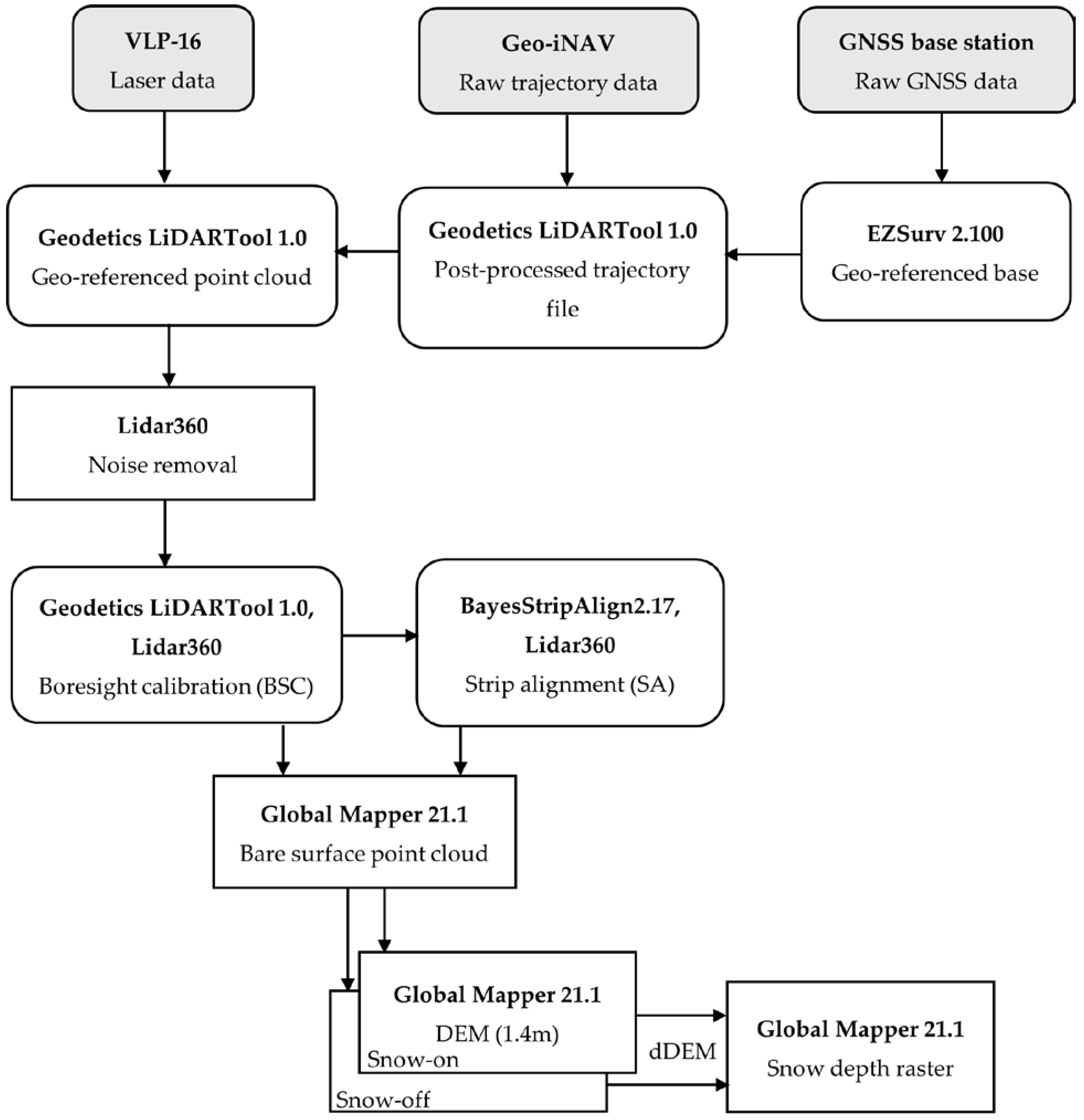
2.3.2. Raw Lidar Data Processing

A geo-referenced lidar point cloud requires post-processing of IMU and GNSS data. First, high-frequency raw trajectory data (x,y,z, heading, pitch, roll) from the Geo-iNAV INS was post-processed in the Geodetics proprietary software LiDARTool [54] with PPK correction. The PPK option regenerates a significantly more accurate trajectory file by correcting the onboard GNSS data with the GNSS base station data [54]. Then, this post-processed trajectory file was merged with the raw laser data to produce a geo-referenced x,y,z point cloud. To reduce the noise level of lidar data, the outer beams of the VLP-16 lidar, where the noise level is highest [54], were discarded from processing (i.e., only the laser beams between ±8° from the full ±15° vertical field of view were used in processing). The outlier removal tool in LiDAR360 [55] removed the remaining low and high noisy data present in lidar data (Figure 5).

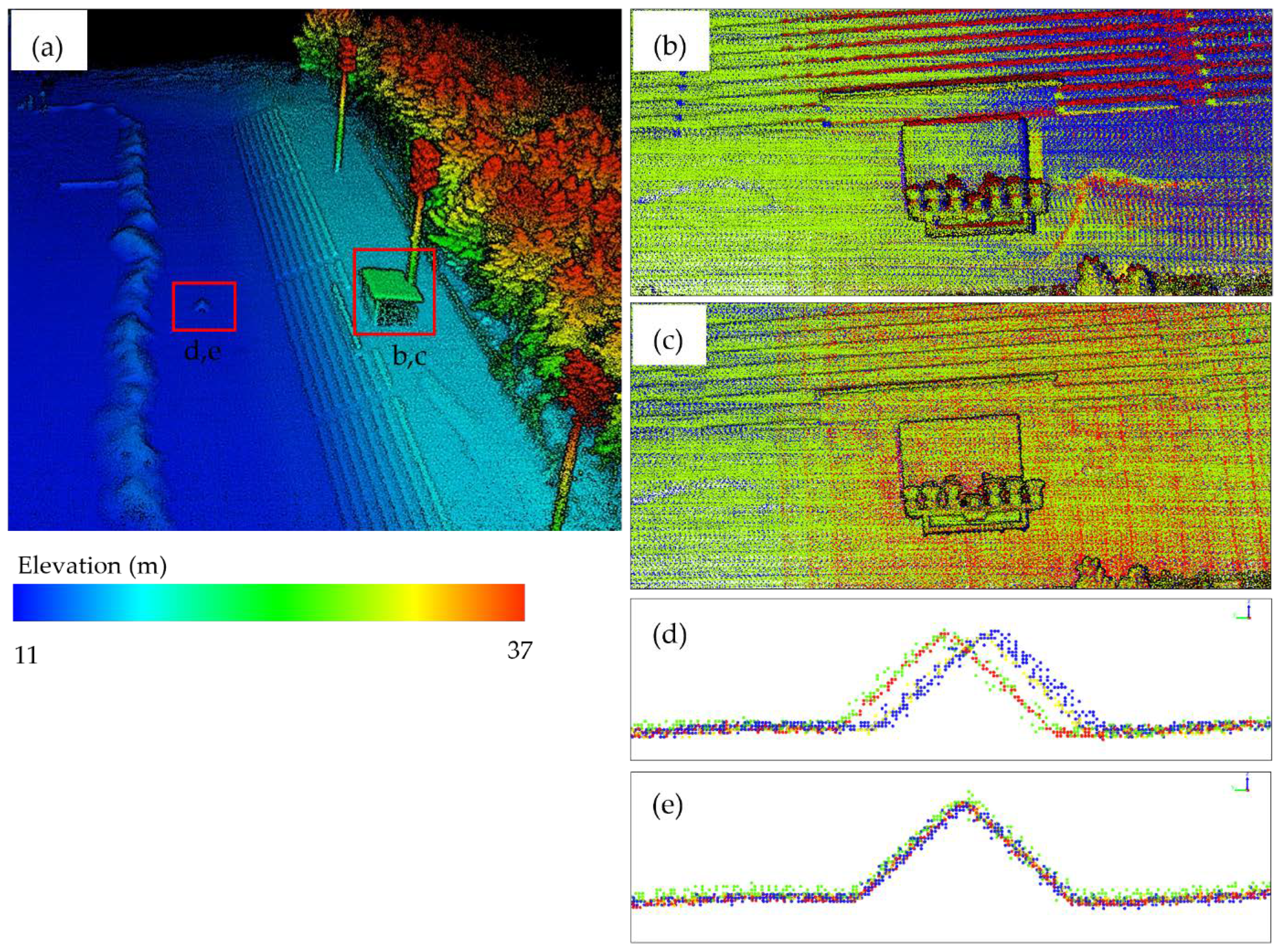
2.3.3. Boresight Calibration

As depicted in Figure 5, while lidar direct geo-referencing with post-processed trajectory and GNSS data is quite precise in the position and orientation of each point cloud, it can be prone to errors if the alignment of the laser sensor to the INS is not precisely known. Quite often, the manufacturer’s calibrated boresight shift and angles of the laser frame to the platform body frame can be slightly offset upon reassembling of the laser sensor on the Geo-iNAV system. This problem can be solved by a boresight calibration. Once calibrated, these values remain constant as long as the lidar sensor payload is not disassembled [54]. For this purpose, we first manually and precisely measured the lever arm distances between the laser sensor and IMU center. To find the boresight angles, the manufacturer recommends a manual adjustment with a trial-and-error procedure [54]. To achieve this, test flights were carried out in the University of Québec at Trois-Rivières premises in April 2019 by flying the Geo-MMS system in different directions over a flat roof and an inclined surface to calibrate the boresight angles (Figure 6a). Processing and visualization of the data collected by the system were carried out in Geodetics LiDARTool and LiDAR360, respectively. The test flights were conducted with the nominal boresight angles (90, 0, −90° in roll, pitch, heading) and the misalignment between flight strips was analyzed in all three rotational axes. Calibration of the boresight angles was initiated with the heading angle. Two opposite direction strips covering the roof edges were selected, plotted together, and the top view alignment was checked. Since the roof edges seem to be misaligned (Figure 6b), the nominal heading angle was increased in a small step of 1° (90, 0, −91° in roll, pitch, heading) and the flight strips were re-processed in LiDARTool. Then, the re-processed flight strips were checked to inspect the impact of the angle change along the roof edges from a top view of the roof. Generally, if two flight strips become more aligned/converged compared with nominal values and if there was still room for convergence, the heading angle was increased in small steps in the same direction (e.g., −92°), otherwise, the angle was increased in the opposite direction (e.g., −89°). Then, the step size was progressively narrowed (e.g., down to 0.1°) when the two strips started converging. This process was continued until a good alignment between flight strips along the heading was achieved (Figure 6c). Once the heading angle was calibrated, and by maintaining the calibrated heading angle, the same procedure was followed to calibrate the pitch and roll angles by checking the misalignment of adjacent flight strips over the inclined surface in the side view in LiDAR360 (Figure 6d,e). The calibrated boresight angles obtained from this procedure for our system were 90.1, 0.28, and −90.6° in roll, pitch, and heading, respectively. Figure 6c,e illustrates the noteworthy improvement of the alignment of the flight strips after boresight calibration. Then, these boresight angle values were used to process data collected from all the flights in this study.

2.3.4. Strip Alignment

We tested an automatic strip alignment algorithm implemented in BayesStripAlign 2.17 software developed by BayesMap solutions, USA, [56] to assess whether it can improve upon the manual boresight calibration procedure. The strip alignment algorithm in BayesStripAlign registers overlapping lidar flight strips and uses relative displacement calculated between those overlapping strips to correct both relative and absolute geometric errors. The goal of the process is to have the smallest possible absolute corrections, while achieving the maximum relative accuracy. The algorithm uses a spatially adaptive approach to address time-dependent effects, such as drifts and oscillations (i.e., high-frequency IMU drifts and oscillations), which cannot be corrected with a classical sensor calibration, and thus effectively reduces the discrepancies between flight strips. Within the algorithm, systematic effects are absorbed by the x and y lever arms, boresight angles, and internal distortion corrections. The high-frequency components of the random walk IMU noise are mainly treated by high-frequency drift corrections. After testing the algorithm with different combinations of aforementioned parameters on the flight strips, the best alignment of overlapping flight strips was found for the automated calibration and correction of the y lever arm, boresight angles, and use of a rigorous model to capture internal distortions and with 5 s intervals for high-frequency drift corrections. This combination of parameters found for our dataset was reviewed and verified by the software developer. BayesStripAlign allows for the control of the absolute accuracy of corrected point cloud using GCP information. The version used in this study includes the automatic detection of GCPs based on local terrain roughness and the calculation of bias using interpolated and gridded lidar data. Each point at GCP locations is weighed using inverse terrain roughness before the absolute accuracy statistics are computed. Unfortunately, the automatic detection of GCPs based on this roughness method did not work well with the elevated GCPs used, and thus this option was excluded from the analysis.

2.3.5. Bare Surface Points Classification

Snow depth mapping requires a classification of the point clouds into the bare surface, ground (from summer survey) or snow (from winter survey). We used the multiscale curvature classification (MCC) algorithm [40] implemented in the commercial Global Mapper software [57] to classify bare surface points. The Global Mapper lidar module identifies possible ground points by employing a morphological filter prior to the application of the MCC algorithm. The morphological filter uses three user-defined parameters of the maximum height difference, expected terrain slope, and maximum building width. MCC uses two user-defined parameters, bin size and minimum height difference from the local mean. Parameters of the algorithm were adjusted according to the vertical spread of the flight strips over open terrain, the local slope of the terrain and streams, and the presence/absence of buildings. A bin size of 0.5 m, a minimum height difference of 0.2 m, a maximum height difference of 10 m, expected terrain slope of 10° in Sainte-Marthe and Saint-Maurice sites and 20° in Montmorency, and a maximum building width of 10 m were found as the optimum parameters for the sites in both seasons. To classify the bare surface points of streams and visible snowbanks, the algorithm was implemented by selecting these areas manually and adjusting the abovementioned parameters to 0.5 m, 0.35–0.45 m, 10 m, 40–70°, and 10 m, respectively. Following a careful inspection of the classified bare surface points, some misclassified points in forested areas were manually reclassified as bare surface.

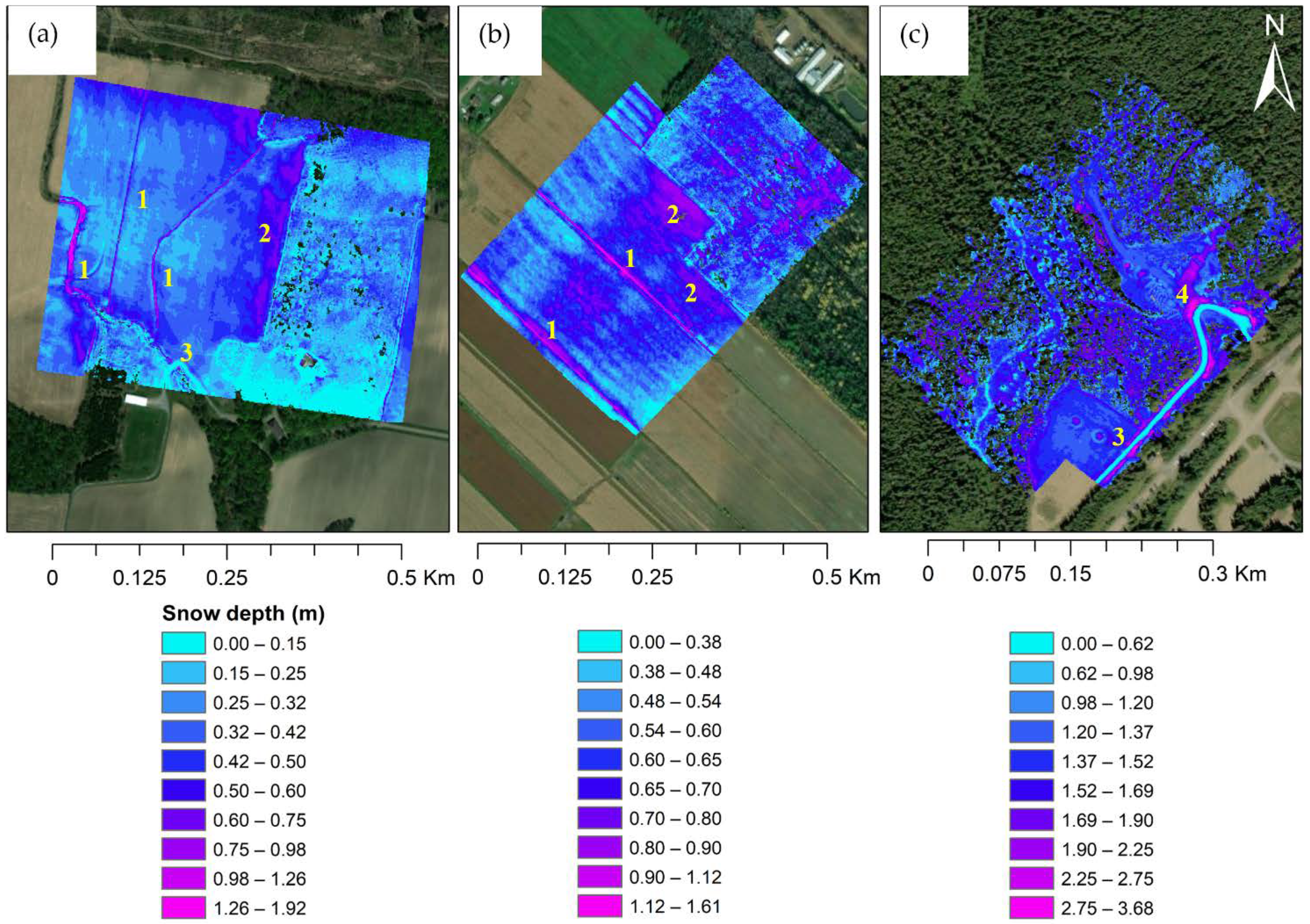
2.3.6. Snow Depth Maps

Snow depth rasters were produced by differencing winter and summer DEMs. DEMs were generated by aggregating bare surface points at each site to a grid resolution of 1.4 m using the binning method in Global Mapper. This method takes the average of the bare surface points that fall inside a grid cell, rather than interpolating. Observation gaps in the point cloud were assigned as no data (i.e., no interpolation method was used to fill the gaps in the DEMs). With the high point density obtained from UAV lidar, this method would ensure that the generated DEMs were of reasonable representations of the true ground/snow surfaces. The grid resolution of 1.4 m was selected based on the manual sampling strategy outlined in Section 2.2.3 (i.e., five measurements at each sampling location represented a 1.4 × 1.4 m ($\sqrt{1^2+1^2}$) grid cell) and aimed at minimizing the effect of GNSS positional errors on manual measurements. As final filtering, spurious negative snow depths were set to zero as they are physically impossible and needed to be filtered out [24]. Negative snow depths were found along the access roads, stream banks, and forested areas. Negative snow depths along access roads could be due to the snow clearing operations in winter. Compressed grasses or shrubs due to snow, and/or misclassification errors, and local changes in topography could be the reason for negative snow depths along stream banks and in forests. However, all these values are rather small in magnitude, accounting for a small portion of the total area (<0.1%) sampled and had a negligible effect on our snow depth statistics. DEMs and snow depth maps derived before applying the strip alignment (i.e., rasters derived after manual boresight calibration only) are denoted as “BSC” and those derived after applying the strip alignment are denoted as “SA”.

2.4. Data Analysis

We assessed the accuracy of UAV lidar in terms of absolute and relative accuracies in the vertical direction (z). The absolute accuracy was determined by comparing the GNSS elevation of the GCPs with those obtained from the lidar data. The relative accuracy between the overlapping flight strips was obtained as a direct output from BayesStripAlign. In addition, one repeat summer flight was conducted on the same day in Sainte-Marthe and used to further assess the spatial distribution of relative errors of the lidar data. The relative accuracy statistics were calculated for the DEM created by differencing the two repeat summer DEMs. The manual snow depth measurements were finally used to validate the lidar-derived snow depth maps. The lidar-derived snow depth error was estimated by comparing each manual measurement to its corresponding 1.4 m grid cell snow depth. The locations of the GCPs and manual measurements are indicated in Figure 1. The error metrics employed to assess accuracies, include the mean (bias), standard deviation (sd), and root mean square error (RMSE).

3. Results

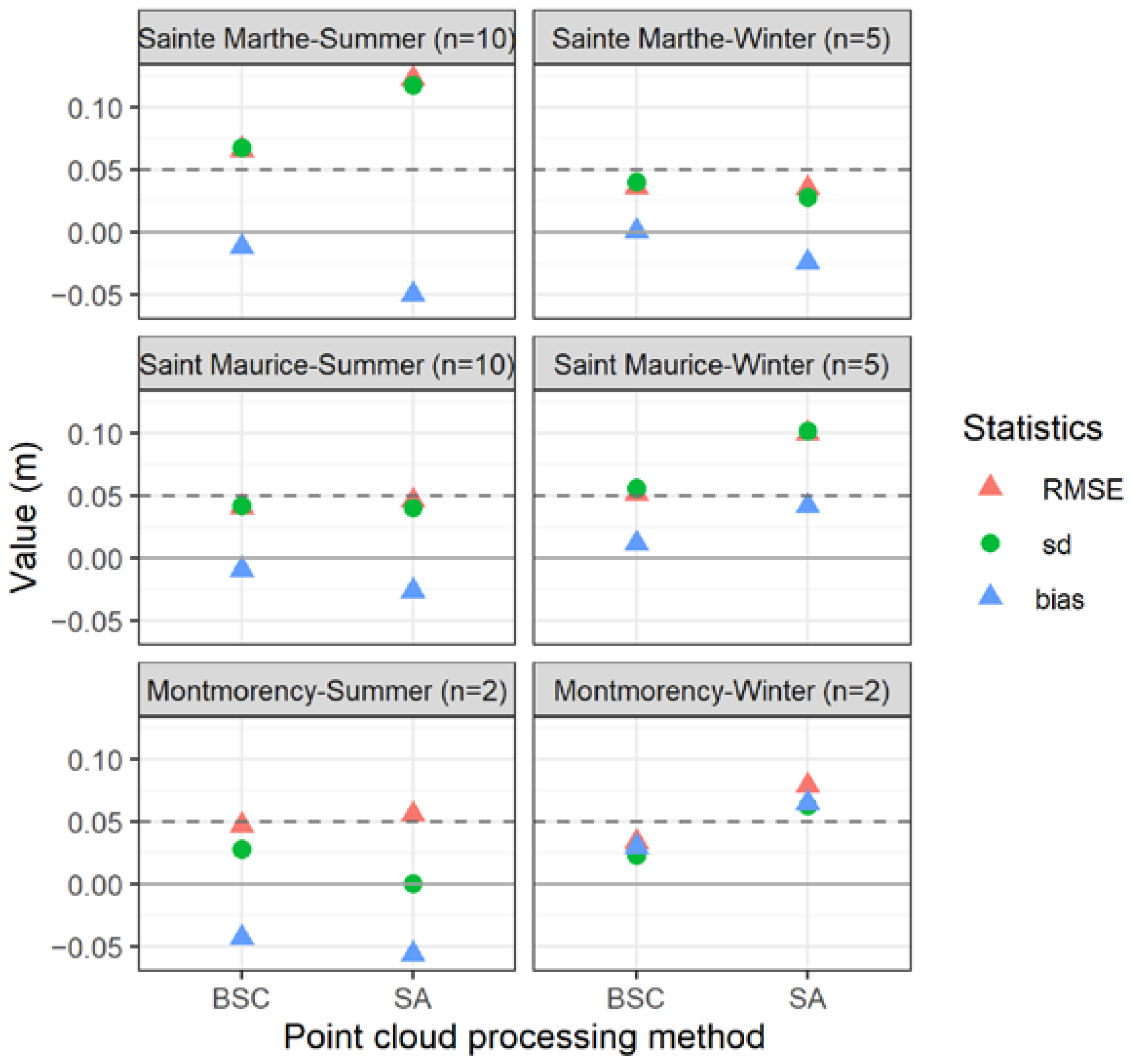
3.1. Accuracy Assessment of Lidar Point Cloud

3.1.1. Absolute Accuracy of Lidar Data

Absolute error statistics calculated for the lidar point cloud are presented in Figure 7. Generally, SA shows an inferior performance, with higher RMSE values than BSC. All BSC results show that the RMSE values are closer to the nominal accuracy of the lidar system (0.05 m), while the majority of the SA RMSE values are higher.

With the BSC method, winter surveys consistently show a lower RMSE, bias, and sd than summer surveys in both Sainte-Marthe and Montmorency. In contrast, the absolute accuracy was slightly better in summer than winter at Saint-Maurice. With the exception of Montmorency, the other two sites generally exhibit a small bias compared with the spread (sd) for both seasons with the BSC method. The SA method exhibits a different pattern: The winter RMSE, bias, and sd are higher at Saint-Maurice and Montmorency than in summer, while Sainte-Marthe shows an opposite tendency. On the other hand, the SA method appears to consistently increase the bias of the BSC data. Moreover, it seems to decrease the summer sd of the BSC data, but increase it in winter, except in Sainte-Marthe.

3.1.2. Relative Accuracy of Lidar Data

The relative RMSE error is a combination of errors from two co-registered point clouds at the same location. The expected uncorrelated relative error for lidar data is approximately 7 cm ($\sqrt{5^2+5^2}$). As seen from Figure 8, SA significantly improved the inter-strip relative accuracy of the BSC data. For example, the large biases in Sainte-Marthe summer and Montmorency winter BSC data were notably reduced after the application of SA. All SA statistics are closer to zero, and well below the nominal error of lidar data.

Repeat flight statistics provide an insight into the probable error values we could expect in snow depth maps, as shown in Figure 9. Accuracy statistics show that relative errors are larger (Figure 9a) and more variable (Figure 9b) in the forested area compared with the field area. SA appears to consistently increase the BSC bias, while decreasing the BSC sd, partly in line with the inter-strip relative statistics found in Figure 8. The estimated RMSE values for the two processing methods in all landscape units are well below the nominal error (Figure 9a).

3.2. Accuracy Assessment of Snow Depth Maps

3.2.1. Lidar-Derived Snow Depth Maps

Snow depth maps were produced for four cases corresponding with the BSC and SA methods and their bias-corrected versions (BSC_BC and SA_BC; BC: Bias-corrected). The bias-corrected DEMs were produced by directly subtracting the bias estimated from the absolute accuracy assessment (Figure 7) to each winter and summer DEM before deriving the snow depth map. Figure 10 shows the snow depth maps derived from UAV lidar data. The overall snow depth patterns among the different processing methods did not significantly differ, thus only the maps from the BSC processing method are shown here.

The highest snow depths are found at the colder and more humid Montmorency site, specifically in forest gaps (Figure 10: Number 4). Higher snow accumulation in streams (Figure 10: Number 1) and along the forest edges (Figure 10: Number 2) is apparent at the two agro-forested sites. Access roads in Sainte-Marthe and Montmorency (Figure 10: Number 3) are snow-free due to snow clearing operations.

3.2.2. Snow Depth Validation

The validation of UAV lidar-derived snow depths with manually sampled ground measurements is shown as boxplots in Figure 11. The boxplots illustrate the discrepancy between the lidar and manual snow depths in the field and forest at each site for the four processing methods, BSC, BSC_BC, SA, and SA_BC.

As seen in Figure 11, boxplots of the Sainte-Marthe field, forest, and Montmorency field show on average a consistent overestimation (positive bias) of lidar snow depths, whereas in Montmorency forest, lidar snow depths seem to be mostly underestimated for all methods. Owing to their different characteristics, field and forest areas in the two sites show contrasting behaviors in terms of lidar snow depth accuracy. In Sainte-Marthe, field snow depths consistently show a higher error dispersion (RMSE = 0.16–0.22 m) than the adjacent deciduous forest (RMSE = 0.079–0.12 m). On the other hand, the small open field in Montmorency exhibits a smaller and less dispersed error (RMSE = 0.043–0.17 m) than the adjacent boreal forest (RMSE = 0.19–0.22 m). The influence of vegetation type is apparent in Figure 11, where the leaf-less deciduous forest in Sainte-Marthe has a smaller RMSE (0.079–0.12 m) compared with evergreen coniferous trees of Montmorency (0.19–0.22 m).

Sainte-Marthe BSC and BSC_BC show a similar performance in both field and forest (Figure 11a,b). This suggests that the small bias of ≤1 cm in each DEM (Figure 7) does not contribute significantly to errors in the final snow depth map. Compared with BSC, SA displays higher RMSE and bias in both field and forest at this site. Despite the slightly better RMSE and bias values of the SA_BC method in comparison with SA, its performance remains inferior to the BSC and BSC_BC methods. In contrast with Sainte-Marthe, BSC_BC shows a lower RMSE and bias in Montmorency field, but a higher RMSE and bias in Montmorency forest, compared with BSC. However, similar to Sainte-Marthe, SA results in a substantial increase in RMSE and bias in the field, but only a minor change in the forest. SA_BC statistics are better than SA in the field, but are still higher than the BSC_BC method. Moreover, the SA_BC method in Montmorency forest shows the highest RMSE and bias among all cases.

4. Discussion

As previously mentioned, error sources in lidar mapping can stem from boresight errors, navigational errors, terrain-induced errors, vegetation-induced errors, and post-processing errors [6,30]. In this study, boresight errors were minimized by a careful boresight calibration. Furthermore, navigational errors posed by the system were minimized by implementing fine alignment (IMU calibration by maneuvering the Geo-MMS through several turns at different velocities prior to the system entering the scanning area [31]), deploying a base station at each site, and using the PPK post-processing technique to correct the Geo-MMS positions. The elevation ranges were small at all sites, as were the slopes (mean grid slopes are 3, 2, and 7° in Sainte-Marthe, Saint-Maurice, and Montmorency, respectively). Therefore, terrain-induced errors are assumed to be minimum. Flight parameters, such as flight height, lidar rotational speed (RPM), overlap, and scan angle were optimized to obtain maximum penetration and minimum occlusion of lidar in the forested area, and thus mitigating errors posed by vegetation. Extensive manual inspection was conducted after each ground point classification to identify any misclassification errors and correct them when necessary. In addition, there could be errors in lidar-derived snow depth products due to changes in microtopography between snow-off and snow-on surveys. For instance, changes of the soil surface due to freezing, possible plowing in agricultural fields, compression of vegetation by snow, and state of understory vegetation could cause spurious and/or negative lidar snow depths [16,17]. Since our snow-off surveys were carried out shortly after the last snowfall with leaf-off deciduous canopy and sub-canopy conditions, and before the growing season begins, it is expected to have minimal changes to the soil surface and minimum effects from vegetation to ground retrievals [10,58]. A good agreement with the lidar-derived snow depths with manually sampled ground measurements in this study implies that these errors, if present, were small overall. Our results demonstrate that while there are still errors in UAV lidar, as with any measuring technique, they are within the expected system accuracy and consistent.

4.1. Comparison of Lidar Point Cloud Accuracy to Previous Studies

Similar to the findings of Harder et al. [16], our BSC absolute accuracy statistics (Figure 7) generally show a better performance in winter. In contrast, SA absolute accuracy statistics showed an inferior performance in winter (except in Sainte-Marthe), most probably due to reduced micro topographical contrasts in the winter point clouds that are used by the strip aligning algorithm to match strip segments. The number of GCPs may also have impacted the accuracy assessment. For example, the use of only two GCPs in Montmorency might not be sufficient to assess the notably high bias observed in Montmorency. Despite this, all BSC results show RMSE values closer to the nominal error of the lidar system (0.05 m), which implies that the collected data were of acceptable accuracy. As expected, SA substantially reduced elevation (z) discrepancies between flight strips. This implies that the application of strip alignment effectively helped in rectifying the misalignment between corresponding segments of overlapping BSC strips. However, the results suggest that this significant improvement in relative accuracy brought by SA was at the cost of the absolute accuracy of lidar data.

Relative error statistics in Figure 9 show that the errors are generally higher and more variable in the forest than in the field area. Lidar data are expected to be more prone to errors in the forest depending on the canopy cover density, the presence of sub-canopy cover, and the lidar ability to penetrate through canopy gaps and reach the ground/snow surface. This observation is analogous to previous studies [16,17], which observed a higher RMSE in the presence of vegetation compared with open areas in their studies. Moreover, Jacobs et al. [17] noted that reduced lidar returns combined with sampling issues contributed to the higher uncertainty of snow depths in the forest compared with open areas in their study.

4.2. Sources of Uncertainty in Lidar-Derived Snow Depths

In general, the snow depth validation error statistics (Figure 11) exhibited higher values than the probable errors estimated from the relative accuracies (Figure 9) across all sites. These higher errors can be explained by site characteristics.

4.2.1. Sainte-Marthe Snow Depths

The higher and more variable snow depth RMSE in the Sainte-Marthe field compared with the adjacent deciduous forest can be explained by the deep, narrow canals/streams in the field (Figure 1 and Figure 10) and the presence of basal ice layers in the snowpack. The notable positive bias in lidar-derived snow depths indicates an overestimation of snow depths by UAV lidar, mostly in the field, as shown by the distinctive higher lidar snow depths for measurements in the area shaded in brown color in Figure 12 (measurement ID 1–31 and 51–56). In contrast, Jacobs et al. [17] and Harder et al. [16] reported slightly low (negative) biases of lidar snow depths compared with manual soundings in a field by UAV lidar in Durham, the United States and Alberta and Saskatchewan, Canada respectively (however, these authors have not reported a presence of basal ice layer in their study sites). As both summer and winter DEMs in this study have biases less than 1 cm, which causes minimal systematic bias in the final snow depth maps, this remaining bias of the lidar snow depths can be attributed to the presence of the ice layers. We observed a 2–10 cm thick ice layer at the base of the snowpack in the field during manual measurements (Figure 2c), which limited the ability of the probe to reach the soil surface. Therefore, in these cases, the lidar measurements are in fact deemed to be more accurate than the manual soundings. As well, as can be observed from Figure 10, snow depths in the streams are twice as deep as the adjacent terrain since snow drifting fills the canals. At locations where the central snow depth manual measurement was directly inside the streams, the average of the five manual measurements was significantly higher or lower than the average lidar snow depths (refer to the range of snow depths at ID 2, 4, 6, 8, 10 in Figure 12), which reflected in higher outlier values (i.e., indicated as “+” in boxplots) of field boxplots in Figure 11a. This is thought to be the main reason for the high variability of errors in the field.

4.2.2. Montmorency Snow Depths

Similar to Sainte-Marthe, Montmorency field lidar snow depths show a positive bias. This could also be due to the presence of an ice layer and the snow tube’s limited penetration ability [17]. Compared with the field, forest lidar snow depth biases are only slightly greater (Sainte-Marthe) and lower (Montmorency) than from the manual soundings in both sites. This contrasts with previous findings from UAV lidar in the forest [16,17,59], where they observed a notable underestimation (negative bias) of lidar snow depths than from the manual measurements compared with the open field. In their studies, the causes of these differences were partially attributed to the snow probe’s ability to penetrate the soil and vegetation, e.g., Jacobs et al. [17] and Proulx et al. [59] suggested that the overprobing by the Magna probe into the thick leaf litter layer present in the forest might have caused the higher average Magna probe snow depths than lidar snow depths. Compared with Sainte-Marthe, Montmorency’s snow depth validation in the coniferous forest does not show a large bias, but a larger dispersion (sd) which increases the RMSE. This larger variation (sd) is attributed to be mainly associated with positional errors caused by multipath effects that are reportedly occurring in areas with thick canopy cover [9,38,51]. Apart from the errors propagated from individual DEMs, misclassification errors in forested areas, and small branches that are compressed by snow can also cause errors in lidar snow depths. However, the higher RMSE in Montmorency has a comparatively smaller impact due to the deeper snowpack observed at the site, i.e., the relative RMSE error (RMSE/mean snow depth) in Montmorency (0.068–0.135) is much lower than the relative error (0.321–0.420) in Sainte-Marthe where the snowpack is shallower.

4.3. Comparison of Lidar Snow Depth Accuracy to Previous Studies

When the strip alignment is not used, the UAV lidar system is able to capture snow depths with a RMSE < 0.16 m in an open environment (including a basal ice layer) and a RMSE < 0.19 m in forests with different canopy covers. This is comparable with previous efforts with UAV lidar (0.09–0.17 m from open to coniferous environment) [16,17] and airborne lidar (0.09–0.35 m from open to coniferous environment) [10,11,12,19,60,61]. Therefore, despite potential inaccuracies within the coniferous forested area, our results show that UAV lidar can be an efficient technique to capture high-resolution, on-demand snow maps within complex agro-forested landscapes.

4.4. Use of GCPs in UAV Lidar

While authors as Harder et al. [16] have suggested that the low bias of UAV lidar errors, without incorporating GCPs, would remove the need of deploying GCPs at the site, we believe that at least a few GCPs are required in natural environments, such as Sainte-Marthe and Saint-Maurice, where distinct manmade structures, such as buildings and roof structures are not present to control for systematic biases in repeat flights. In these environments, GCPs would ensure an absolute check of the lidar dataset and provide a quantitative assessment of the bias, and thus would help in correcting the bias of the data. Csanyi and Toth [62] also highlighted the importance of using well-defined lidar-specific GCPs for applications with high accuracy requirements (e.g., survey-grade mapping). They showed that using specifically designed lidar targets (1 m radius circular-shaped elevated targets) could improve the lidar flight strip accuracies. Furthermore, they mentioned that in the absence of three-dimensional ground information, such as buildings and roof structures at site, the information from mobile lidar specific ground control targets can be used in or after the strip adjustment process to correct the remaining absolute errors in the corrected strips.

4.5. Use of Strip Alignment for UAV Lidar

Our results showed that while the SA algorithm improved the relative accuracy of the point clouds, its ultimate impact was to degrade the snow depth validation compared with the simple BSC method, even after bias correction. This observation was consistent in both field and forested areas, and at all sites. Possible reasons for this inferior performance can be attributed to the limitations of the algorithm used. The software version did not support the elevated GCPs used in this study, and thus did not use the GCP information during strip alignment, which led to degrading the absolute errors of the point cloud. It is not surprising that the SA exacerbated errors in winter, as there were fewer or no microtopographic features for the strip aligning algorithm to match the point cloud segments reliably in winter. Therefore, our results indicate that the SA implemented in this study is not suitable for similar UAV lidar applications, especially for monitoring snow depths. The main reason for using BayesStripAlign was for its ability to directly use the las and trajectory files rather than raw data from the laser scanner [21], which is not currently retrievable from the Geo-MMS system. However, our results could be used to improve the BayesStripAlign SA algorithm for further UAV applications in snow-covered landscapes.

5. Conclusions

This study demonstrated the ability of UAV lidar to measure snow depth variability under varying vegetation covers with reasonable accuracy. However, the observation gaps in ground returns in the coniferous forest imply that, despite the higher point density returned by the UAV lidar compared with ALS, airborne remote sensing techniques alone are not able to retrieve a comprehensive snow depth distribution pattern under a coniferous canopy. A combination of UAV lidar and ground-based manual measurement (or under and above canopy UAV lidar as demonstrated by Hyyppä et al. [63]) might be beneficial to obtain more representative and extensive snow depths in coniferous environments.

The results showed that the strip alignment approach we used was not suitable for UAV lidar, since it degraded the absolute accuracy of the point clouds. The dataset would potentially benefit from a strip alignment algorithm that incorporates GCPs in the alignment procedure and/or uses that information in a 3D (x,y,z) adjustment of the point cloud.

Nevertheless, it can be concluded from the results that a careful boresight calibration can provide centimeter-level accuracy of lidar data without SA enhancement. Therefore, boresight calibration should receive paramount attention in the data processing workflow. Moreover, a well-formulated flight plan plays a critical role in reducing system errors. Utilizing two or more turning maneuvers allows for better tuning of the IMU. Furthermore, flying at a lower altitude and slower speed reduces the impact of uncertainty in the boresight angles. Flight planning should also address weather conditions, for instance, flying the Geo-MMS in windy conditions (wind speeds higher than 8 m/s according to specifications) would degrade the sensor accuracies. The deployment of GCPs ensures an absolute check of data in the absence of distinct structures visible from airborne sensors. Importantly, a successful ground point classification is critical to the final accuracy of the snow depth maps. A manual inspection of the geo-referenced point cloud is advisable following automatic classification, preferably with geo-tagged imagery if available.

The methodological framework presented in this paper provides a valuable contribution to the UAV lidar accuracy assessments for snow research, which is reproducible in similar environments.

References

1. Barnett, T.P.; Adam, J.C.; Lettenmaier, D.P. Potential impacts of a warming climate on water availability in snow-dominated regions. Nature 2005, 438, 303–309. [Google Scholar] [CrossRef] [PubMed]
2. Clark, M.; Hendrikx, J.; Slater, A.; Kavetski, D.; Anderson, B.; Cullen, N.J.; Kerr, T.; Hreinsson, E.; Woods, R. Representing spatial variability of snow water equivalent in hydrologic and land surface models: A review. Water Resour. Res. 2011, 47, W07539. [Google Scholar] [CrossRef] [Green Version]
3. Sturm, M.; Goldstein, M.A.; Parr, C. Water and life from snow: A trillion dollar science question. Water Resour. Res. 2017, 53, 3534–3544. [Google Scholar] [CrossRef]
4. NSIDC. State of the Cryosphere. Available online: https://nsidc.org/cryosphere/sotc/ (accessed on 20 October 2020).
5. Aygün, O.; Kinnard, C.; Campeau, S. Impacts of climate change on the hydrology of northern midlatitude cold regions. Prog. Phys. Geogr. Earth Environ. 2020, 44, 338–375. [Google Scholar] [CrossRef]
6. Deems, J.S.; Painter, T.H.; Finnegan, D.C. Lidar measurement of snow depth: A review. J. Glaciol. 2013, 59, 467–479. [Google Scholar] [CrossRef] [Green Version]
7. Dong, C. Remote sensing, hydrological modeling and in situ observations in snow cover research: A review. J. Hydrol. 2018, 561, 573–583. [Google Scholar] [CrossRef]
8. Tsai, Y.-L.S.; Dietz, A.; Oppelt, N.; Kuenzer, C. Remote sensing of snow cover using spaceborne SAR: A review. Remote Sens. 2019, 11, 1456. [Google Scholar] [CrossRef] [Green Version]
9. Hopkinson, C.; Pomeroy, J.; Debeer, C.; Ellis, C.; Anderson, A. Relationships between snowpack depth and primary lidar point cloud derivatives in a mountainous environment. In Proceedings of the Remote Sensing and Hydrology, Jackson Hole, WY, USA, 27–30 September 2010. [Google Scholar]
10. Hopkinson, C.; Sitar, M.; Chasmer, L.; Treitz, P. Mapping snowpack depth beneath forest canopies using airborne lidar. Photogramm. Eng. Remote Sens. 2004, 70, 323–330. [Google Scholar] [CrossRef] [Green Version]
11. Harpold, A.A.; Guo, Q.; Molotch, N.; Brooks, P.D.; Bales, R.; Fernandez-Diaz, J.C.; Musselman, K.N.; Swetnam, T.L. Lidar-derived snowpack data sets from mixed conifer forests across the Western United States. Water Resour. Res. 2014, 50, 2749–2755. [Google Scholar] [CrossRef] [Green Version]
12. Zheng, Z.; Kirchner, P.B.; Bales, R.C. Topographic and vegetation effects on snow accumulation in the southern Sierra Nevada: A statistical summary from lidar data. Cryosphere 2016, 10, 257–269. [Google Scholar] [CrossRef] [Green Version]
13. Zheng, Z.; Ma, Q.; Qian, K.; Bales, R.C. Canopy effects on snow accumulation: Observations from lidar, canonical-view photos, and continuous ground measurements from sensor networks. Remote Sens. 2018, 10, 1769. [Google Scholar] [CrossRef] [Green Version]
14. Currier, W.R.; Lundquist, J.D. Snow depth variability at the forest edge in multiple climates in the western United States. Water Resour. Res. 2018, 54, 8756–8773. [Google Scholar] [CrossRef]
15. Mazzotti, G.; Currier, W.; Deems, J.S.; Pflug, J.M.; Lundquist, J.D.; Jonas, T. Revisiting snow cover variability and canopy structure within forest stands: Insights from airborne lidar data. Water Resour. Res. 2019, 55, 6198–6216. [Google Scholar] [CrossRef]
16. Harder, P.; Pomeroy, J.; Helgason, W. Improving sub-canopy snow depth mapping with unmanned aerial vehicles: Lidar versus structure-from-motion techniques. Cryosphere 2020, 14, 1919–1935. [Google Scholar] [CrossRef]
17. Jacobs, J.M.; Hunsaker, A.G.; Sullivan, F.B.; Palace, M.; Burakowski, E.A.; Herrick, C.; Cho, E. Snow depth mapping with unpiloted aerial system lidar observations: A case study in Durham, New Hampshire, United States. Cryosphere 2021, 15, 1485–1500. [Google Scholar] [CrossRef]
18. Morsdorf, F.; Kötz, B.; Meier, E.; Itten, K.I.; Allgöwer, B. Estimation of LAI and fractional cover from small footprint airborne laser scanning data based on gap fraction. Remote Sens. Environ. 2006, 104, 50–61. [Google Scholar] [CrossRef]
19. Painter, T.; Berisford, D.; Boardman, J.; Bormann, K.J.; Deems, J.; Gehrke, F.; Hedrick, A.; Joyce, M.; Laidlaw, R.; Marks, D.; et al. The Airborne Snow Observatory: Fusion of scanning lidar, imaging spectrometer, and physically-based modeling for mapping snow water equivalent and snow albedo. Remote Sens. Environ. 2016, 184, 139–152. [Google Scholar] [CrossRef] [Green Version]
20. Broxton, P.D.; Harpold, A.A.; Biederman, J.A.; Troch, P.A.; Molotch, N.P.; Brooks, P.D. Quantifying the effects of vegetation structure on snow accumulation and ablation in mixed-conifer forests. Ecohydrology 2015, 8, 1073–1094. [Google Scholar] [CrossRef]
21. Glira, P.; Pfeifer, N.; Mandlburger, G. Rigorous strip adjustment of UAV-based laserscanning data including time-dependent correction of trajectory errors. Photogramm. Eng. Remote Sens. 2016, 82, 945–954. [Google Scholar] [CrossRef] [Green Version]
22. Pajares, G. Overview and current status of remote sensing applications based on Unmanned Aerial Vehicles (UAVs). Photogramm. Eng. Remote Sens. 2015, 81, 281–329. [Google Scholar] [CrossRef] [Green Version]
23. Michele, C.; Avanzi, F.; Passoni, D.; Barzaghi, R.; Pinto, L.; Dosso, P.; Ghezzi, A.; Gianatti, R.; Vedova, G.D. Using a fixed-wing UAS to map snow depth distribution: An evaluation at peak accumulation. Cryosphere 2016, 10, 511–522. [Google Scholar] [CrossRef] [Green Version]
24. Hopkinson, C.; Collins, T.; Anderson, A.; Pomeroy, J.; Spooner, I. Spatial snow depth assessment using lidar transect samples and public GIS data layers in the Elbow River watershed, Alberta. Can. Water Resour. J. 2012, 37, 69–87. [Google Scholar] [CrossRef]
25. Deems, J.S.; Fassnacht, S.R.; Elder, K.J. Fractal distribution of snow depth from lidar data. J. Hydrometeorol. 2006, 7, 285–297. [Google Scholar] [CrossRef]
26. Trujillo, E.; Ramírez, J.A.; Elder, K.J. Topographic, meteorologic, and canopy controls on the scaling characteristics of the spatial distribution of snow depth fields. Water Resour. Res. 2007, 43, W07409. [Google Scholar] [CrossRef]
27. Kirchner, P.B.; Bales, R.C.; Molotch, N.P.; Flanagan, J.; Guo, Q. Lidar measurement of seasonal snow accumulation along an elevation gradient in the southern Sierra Nevada, California. Hydrol. Earth Syst. Sci. 2014, 18, 4261–4275. [Google Scholar] [CrossRef] [Green Version]
28. Li, Z.; Tan, J.; Liu, H. Rigorous boresight self-calibration of mobile and UAV LiDAR scanning systems by strip adjustment. Remote Sens. 2019, 11, 442. [Google Scholar] [CrossRef] [Green Version]
29. Gatziolis, D.; Andersen, H.-E. A Guide to Lidar Data Acquisition and Processing for the Forests of the Pacific Northwest; United States Department of Agriculture: Portland, OR, USA, 2008.
30. Pilarska, M.; Ostrowski, W.; Bakula, K.; Górski, K.; Kurczynski, Z. The potential of light laser scanners developed for unmanned aerial vehicles-The review and accuracy. ISPRS Int. Arch. Photogramm. Remote Sens. Spat. Inf. Sci. 2016, 42, 87–95. [Google Scholar] [CrossRef] [Green Version]
31. Geodetics, I. Geo-MMS User Manual (Document 20160 Rev B); Geodetics, Inc.: San Diego, CA, USA, 2019. [Google Scholar]
32. Zhang, X.; Gao, R.; Sun, Q.; Cheng, J. An automated rectification method for unmanned aerial vehicle LiDAR point cloud data based on laser intensity. Remote Sens. 2019, 11, 811. [Google Scholar] [CrossRef] [Green Version]
33. Ravi, R.; Shamseldin, T.; Elbahnasawy, M.; Lin, Y.-J.; Habib, A. Bias impact analysis and calibration of UAV-based mobile LiDAR system with spinning multi-beam laser scanner. Appl. Sci. 2018, 8, 297. [Google Scholar] [CrossRef] [Green Version]
34. De Oliveira Junior, E.M.; Dos Santos, D.R. Rigorous calibration of UAV-based LiDAR systems with refinement of the boresight angles using a point-to-plane approach. Sensors 2019, 19, 5224. [Google Scholar] [CrossRef] [Green Version]
35. Glira, P.; Pfeifer, N.; Briese, C.; Ressl, C. A correspondence framework for ALS strip adjustments based on variants of the ICP algorithm. J. Photogramm. Remote Sens. Geoinf. Sci. 2015, 4, 275–289. [Google Scholar] [CrossRef]
36. Kumari, P.; Carter, W.E.; Shrestha, R.L. Adjustment of systematic errors in ALS data through surface matching. Adv. Space Res. 2011, 47, 1851–1864. [Google Scholar] [CrossRef]
37. Chen, Z.; Li, J.; Yang, B. A strip adjustment method of UAV-borne lidar point cloud based on DEM features for mountainous area. Sensors 2021, 21, 2782. [Google Scholar] [CrossRef]
38. Hyyppä, H.; Hyyppä, J.; Kaartinen, H.; Kaasalainen, S.; Honkavaara, E.; Rönnholm, P. Factors affecting the quality of DTM generation in forested areas. In Proceedings of the ISPRS Workshop Laser Scanning 2005, Enschede, The Netherlands, 12–14 September 2005; pp. 85–90. [Google Scholar]
39. Wallace, L.O.; Lucieer, A.; Watson, C.S. Assessing the feasibility of UAV-based lidar for high resolution forest change detection. In Proceedings of the ISPRS Congress, Melbourne, Australia, 25 August–1 September 2012; pp. 499–504. [Google Scholar]
40. Evans, J.S.; Hudak, A.T. A multiscale curvature algorithm for classifying discrete return LiDAR in forested environments. IEEE Trans. Geosci. Remote Sens. 2007, 45, 1029–1038. [Google Scholar] [CrossRef]
41. Yilmaz, C.S.; Yilmaz, V.; Güngör, O. Investigating the performances of commercial and non-commercial software for ground filtering of UAV-based point clouds. Int. J. Remote Sens. 2018, 39, 5016–5042. [Google Scholar] [CrossRef]
42. Aygün, O.; Kinnard, C.; Campeau, S.; Krogh, S.A. Shifting hydrological processes in a Canadian agroforested catchment due to a warmer and wetter climate. Water 2020, 12, 739. [Google Scholar] [CrossRef] [Green Version]
43. Jobin, B.; Latendresse, C.; Baril, A.; Maisonneuve, C.; Boutin, C.; Côté, D. A half-century analysis of landscape dynamics in southern Québec, Canada. Environ. Monit. Assess. 2014, 186, 2215–2229. [Google Scholar] [CrossRef]
44. Paquotte, A.; Baraer, M. Hydrological behavior of an ice-layered snowpack in a non-mountainous environment. Hydrol. Processes 2021, 36, e14433. [Google Scholar] [CrossRef]
45. Royer, A.; Roy, A.; Jutras, S.; Langlois, A. Review article: Performance assessment of radiation-based field sensors for monitoring the water equivalent of snow cover (SWE). Cryosphere 2021, 15, 5079–5098. [Google Scholar] [CrossRef]
46. Environment and Climate Change Canada. Canadian Climate Normals 1981–2010, Edited. Available online: https://climate.weather.gc.ca/ (accessed on 10 August 2020).
47. VelodyneLiDAR. VLP-16 User Manual; Velodyne LiDAR, Inc.: San Jose, CA, USA, 2018. [Google Scholar]
48. Geodetics, I. Geo-iNAV®,Geo-RelNAV®,Geo-PNT®,Geo-Pointer™,Geo-hNAV™,Geo-MMS™ and Geo-RR™ Commercial User Manual (Document 20134 Rev X); Geodetics, Inc.: San Diego, CA, USA, 2018. [Google Scholar]
49. SPH-Engineering. UgCS Desktop Application Version 3.2 (113) User Manual; SPH Engineering: Baložu Pilsēta, Latvia, 2019. [Google Scholar]
50. Sturm, M.; Holmgren, J. An automatic snow depth probe for field validation campaigns. Water Resour. Res. 2018, 54, 9695–9701. [Google Scholar] [CrossRef]
51. Valbuena, R.; Mauro, F.; Rodriguez-Solano, R.; Manzanera, J.A. Accuracy and precision of GPS receivers under forest canopies in a mountainous environment. Span. J. Agric. Res. 2010, 8, 1047–1057. [Google Scholar] [CrossRef]
52. Effigis. EZSurv User Manual; Effigis: Montreal, QC, Canada, 2019. [Google Scholar]
53. Ministry of Energy and Natural Resources. Geodetic Network Map. Available online: https://geodesie.portailcartographique.gouv.qc.ca/ (accessed on 5 February 2019).
54. Geodetics, I. LiDARTool™ User Manual (Document 20149 Rev I); Geodetics, Inc.: San Diego, CA, USA, 2019. [Google Scholar]
55. GreenValley-International. LiDAR360 User Guide; GreenValley International, Ltd.: Berkeley, CA, USA, 2020. [Google Scholar]
56. Bayesmap Solutions. BayesStripAlign 2.1 Software Manual; BayesMap Solutions, LLC.: Mountain View, CA, USA, 2020. [Google Scholar]
57. Blue Marble Geographics. Global Mapper; Blue Marble Geographics: Hallowell, ME, USA, 2020. [Google Scholar]
58. Evans, J.; Hudak, A.T.; Faux, R.; Smith, A.M.S. Discrete return lidar in natural resources: Recommendations for project planning, data processing, and deliverables. Remote Sens. 2009, 1, 776–794. [Google Scholar] [CrossRef] [Green Version]
59. Proulx, H.; Jacobs, J.M.; Burakowski, E.A.; Cho, E.; Hunsaker, A.G.; Sullivan, F.B.; Palace, M.; Wagner, C. Comparison of in-situ snow depth measurements and impacts on validation of unpiloted aerial system lidar over a mixed-use temperate forest landscape. Cryosphere Discuss 2022, 2022, 1–20. [Google Scholar] [CrossRef]
60. Broxton, P.; Leeuwen, W.J.V.; Biederman, J. Improving snow water equivalent maps with machine learning of snow survey and lidar measurements. Water Resour. Res. 2019, 55, 3739–3757. [Google Scholar] [CrossRef]
61. Tinkham, W.T.; Smith, A.M.S.; Marshall, H.; Link, T.; Falkowski, M.; Winstral, A. Quantifying spatial distribution of snow depth errors from lidar using random forest. Remote Sens. Environ. 2014, 141, 105–115. [Google Scholar] [CrossRef]
62. Csanyi, N.; Toth, C.K. Improvement of lidar data accuracy using lidar-specific ground targets. Photogramm. Eng. Remote Sens. 2007, 73, 385–396. [Google Scholar] [CrossRef] [Green Version]
63. Hyyppä, E.; Hyyppä, J.; Hakala, T.; Kukko, A.; Wulder, M.A.; White, J.C.; Pyörälä, J.; Yu, X.; Wang, Y.; Virtanen, J.-P.; et al. Under-canopy UAV laser scanning for accurate forest field measurements. ISPRS J. Photogramm. Remote Sens. 2020, 164, 41–60. [Google Scholar] [CrossRef]
Figure 1. Overview of the study sites with lidar survey extents. (a) Sainte-Marthe; (b) Saint-Maurice; and (c) Montmorency. Manual measurement and ground control point (GCP) locations are also shown. (Manual measurements in Saint-Maurice could not be retrieved due to a probe malfunctioning, thus they are not shown). Contour intervals deliberately differed between sites for interpretation purposes.
Remotesensing 14 01649 g001
Figure 2. (a) Sainte-Marthe site during summer survey and (b) during winter survey; (c) presence of basal ice layer in Sainte-Marthe field; (d) Saint-Maurice site during summer survey and (e) during winter survey; (f) Montmorency site during summer survey and (g) during winter survey; (h) local snow accumulation in a forest gap in Montmorency boreal forest.
Remotesensing 14 01649 g002
Figure 3. UAV lidar system.
Remotesensing 14 01649 g003
Figure 4. Manmade GCPs: (a) Elevated and (b) flat. Photos were taken after the lidar surveys with FOIF A30 GNSS receiver on the target surface.
Remotesensing 14 01649 g004
Figure 5. Data processing workflow of lidar data. Each box shows the software used (bold) with the corresponding end product.
Remotesensing 14 01649 g005
Figure 6. An example plot of the boresight calibration procedure. (a) 3D view of the calibration site, lidar point cloud is colorized by elevation (roof structure and inclined surface are demarcated in red squares with relevant letters); (b) top view of the roof structure for nominal boresight angles and (c) for calibrated boresight angles; (d) cross-section view of the inclined surface for nominal boresight angles and (e) for calibrated boresight angles. Points scanned from different strips have different colors (red, blue, yellow, and green).
Remotesensing 14 01649 g006
Figure 7. Absolute error statistics of lidar point clouds. Plots are segmented by site (rows), data processing method (columns), and error statistics (colors). The grey dashed line is the expected accuracy of the lidar system. n denotes the number of GCPs. BSC: Boresight calibrated point cloud; SA: Boresight + strip-aligned point cloud. (Bias was calculated as lidar-derived DEM elevation − GNSS elevation at GCPs).
Remotesensing 14 01649 g007
Figure 8. Relative error statistics between overlapping flight strips.
Remotesensing 14 01649 g008
Figure 9. (a) Relative error statistics from repeat flights in field, forest, and the combined landscape for the two point cloud processing methods; (b) relative error distribution in field, forest, and the combined landscape of the BSC data.
Remotesensing 14 01649 g009
Figure 10. UAV lidar-derived snow depth maps. (a) Sainte-Marthe; (b) Saint-Maurice; and (c) Montmorency. Features 1 to 4 are discussed in the text.
Remotesensing 14 01649 g010
Figure 11. Distribution of the differences between lidar and manual snow depth for the different point cloud processing methods. (a) Sainte-Marthe field; (b) Sainte-Marthe forest; (c) Montmorency field; and (d) Montmorency forest. BSC: Boresight calibrated point cloud; SA: Boresight + strip-aligned point cloud; BSC_BC: Bias-corrected BSC data; SA_BC: Bias-corrected SA data. Outliers are indicated by “+” symbol in boxplots.
Remotesensing 14 01649 g011
Figure 12. Variability of manual and lidar snow depth measurements in Sainte-Marthe. Error bars represent the minimum and maximum snow depth values of the five manual measurements taken at each sampling location and blue dots denote the average value of the five measurements. Measurements in the field (ID 1–31 and 51–56) and the forest (ID 32–50) are demarcated by brown and green colored shadings, respectively.
Remotesensing 14 01649 g012