HD Camera-Equipped UAV Trajectory Planning for Gantry Crane Inspection

Abstract

While Unmanned Aerial Vehicles (UAVs) can be a valuable solution for the damage inspection of port machinery infrastructures, their trajectories are still prone to collision risks, trajectory non-smoothness, and large deviations. This research introduces a trajectory optimization method for inspecting vulnerable parts of a gantry crane by a UAV fitted with a high-definition (HD) camera. We first analyze the vulnerable parts of a gantry crane, then use the A* algorithm to plan a path for the UAV. The trajectory optimization process is divided into two steps, the first is a trajectory correction method and the second is an objective function that applies a minimum snap method while taking into consideration flight corridor constraints. The experimental simulation results show that, compared with previous methods, our approach can not only generate a collision-free and smooth trajectory but also shorten the trajectory length significantly while substantially reducing the maximum deviation average deviation distances. The simulation results show that this modelling approach provides a valuable solution for UAV trajectory planning for gantry crane inspection.

1. Introduction

A gantry crane is a common and large port hoisting equipment for loading and unloading goods. During regular hoisting operations, a gantry crane faces regular vibration impacts caused by a strong dynamic load, leading to performance degradation or even sudden failure under long-term actions. Therefore, and to maintain the quality of port operations, there is a need to conduct regular and comprehensive port machinery inspections.

Over the past few years, UAVs have been widely used thanks to their small size, light weight, low cost, and ability to carry out various inspections in complex environments [1]. Damage inspections have been widely used on many engineering and building infrastructures such as bridge with crack in [2], reinforced concrete with cracks in [3] and quay cranes with structural damage [4]. A UAV equipped with a camera appears to be a flexible, efficient, and economical method [5,6].

The research developed in this paper introduces a trajectory optimization method for the inspection of vulnerable points of a gantry crane using a UAV equipped with an HD camera. Our modelling approach first takes into consideration the specific properties and vulnerable parts of a gantry crane, then determines the key UAV trajectory points that will perform the inspection tasks. A UAV trajectory planning for inspecting the vulnerable points of a gantry crane should find an optimized flight trajectory from start to finish that can also avoid all obstacles. Our proposed approach is made of two parts. The first part is the path planning algorithm whose objective is to theoretically generate straight paths between inspection points. The second part is trajectory planning, which uses the method of constructing the minimization objective function based on minimum snap to generate a continuous trajectory for the UAV. Then, to solve the deviation of the UAV trajectory, the first step is to use the trajectory correction method to solve the deviation of the UAV at the corner. The second step is to use the flight corridor method to limit the UAV trajectory within an appropriate framework to generate a smoother and safer trajectory. Experiments of the whole approach are conducted using a simulation environment whose objectives are to evaluate performance figures. The UAV can realize automatic inspection. This improves the efficiency and safety of a UAV patrol inspection and management efficiency. This approach can be applied to the inspection of multiple port cranes. The rest of the paper is structured as follows. First, Section 2 introduces our methodology and the problem statement while Section 3 develops the simulation results. Finally, Section 4 discusses the findings and Section 5 concludes the paper.

2. Methodology and Problem Statement

2.1. Methodology

Maintaining flight efficiency and control of a UAV is a non-straightforward task. Different control technologies have been implemented such as proportional integral differential [7], linear quadratic regulator [8], active disturbance rejection control [9], robust control [10,11], and some nonlinear control methods [12,13]. When the mission of UAV is simple, common linear control methods can stabilize UAV trajectory. However, if a large working range is considered, such as plant protection or patrol inspection, the performance of the linear controller is likely to decrease. This favors the development of nonlinear methods with a nonlinear controller under the condition of parameter uncertainty and unknown external interference as suggested by Zhao et al. [14]. The proposed controller can perform an asymptotic tracking of a time-varying reference trajectory and then control the stability of the UAV.

UAV path planning methods have attracted a significant number of works such as genetic algorithm [15], Dijkstra algorithm [16], A* algorithm [17], RRT algorithm [18], and RRT* algorithm [19]. A genetic algorithm is designed and put forward according to the evolution law of living organisms. Dijkstra algorithm is the shortest path algorithm from one vertex to other vertices, which solves the shortest path problem in weighted graph. The A* algorithm has been proven as the most effective direct search method to solve the shortest path in a given road network and is also an effective algorithm to solve many search problems. RRT algorithm is a sampling based method, which is relatively effective. It can quickly plan a path, but the path is not optimal. RRT * algorithm is an improved version of RRT algorithm, which can get the asymptotic optimal solution, but the search time is too long. A UAV flight path planning method has been proposed and based on the bat algorithm and integrated into an artificial bee colony algorithm [20]. However, it has been proved that these algorithms suffer from many problems such as the lack of solution accuracy, smooth path, and the likely possibility of falling into local optimization. An artificial potential field method updated by optimal control theory generates relatively short and smooth trajectories [21]. However, defining the potential field precisely is a difficult task.

Different trajectory optimization methods such as the Bezier curve [22], B-spline curve [23], and minimum snap [24] have so far been suggested by previous works. A path planning method combining the A* algorithm and Bezier curve has been suggested to solve the problem of large-angles and many broken lines [25]. However, the Bezier curve lacks local flexibility, that is, changing a control point has an impact on the whole curve. A dynamic UAV re-planning based on a B-spline curve has been proposed [26], one that can effectively deal with the problem of non-static UAV paths, but this method is computationally heavy. The minimum snap method is a suitable choice for the four-rotor UAV with multiple degrees of freedom, and the minimum snap polynomial spline has been proved to be very effective as the trajectory of UAV, which can ensure the quality of the measurement data of UAV airborne sensors. However, this method also has some limitations, when a multi-stage trajectory is involved, the optimization method still has issues to resolve. To solve the above problems, unconstrained quadratic programming can be applied. An improved trajectory optimization method can be applied to continuous multi-stage trajectories [27], but these methods do not take into consideration whether the smoothness properties of the generated trajectory or the deviation degree are low. This leads us to combine an A* path planning with a trajectory optimization based on an objective function that applies a minimum snap method to consider flight corridor constraints. The objective is to inspect the vulnerable parts of the gantry crane using a UAV equipped with a high-definition camera.

2.2. Problem Statement

Correct path planning and trajectory optimization can generate a high-quality trajectory for a UAV. The goal of UAV path planning is to find a short collision-free path, whereas the goal of trajectory optimization is to find the collision-free and smooth trajectory to ensure efficient UAV inspections.

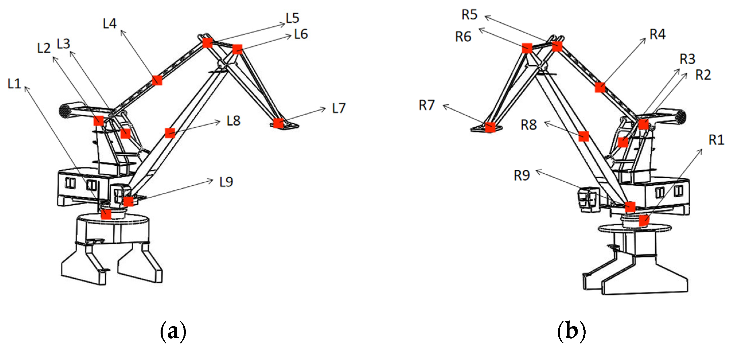
2.2.1. Gantry Crane Vulnerable Parts

A gantry crane is a relatively complex port machinery system. During a crane’s frequent operations, some parts can be easily damaged. Fatigue damage is the main form of failure of the metal structure of port cranes. According to the loading test and experience of relevant experts, the vulnerable parts of the gantry crane can be obtained. Figure 1 shows the vulnerable parts on the left and right sides of a relevant example of a gantry crane, in which the red marks denote the vulnerable parts. Due to the symmetry of the crane, L and R are used to represent the vulnerable points on the left and right sides; among them, L1 to L9 represent 9 vulnerable points on the left side of the gantry crane, while R1 to R9 represent 9 vulnerable points on the right side of the gantry crane.

According to Figure 1, the vulnerable parts of the gantry crane are mainly the connections between the balance beam and counterweight, the upper end of the boom, the middle of the small pull rod, the upper end, the lower end of the large pull rod, the two ends of nose beam, and the rest of the damage is to the metal and non-metal parts of the gantry crane.

The gantryl crane is modeled. In this state, the crane does not load goods and the boom is raised, as shown in Figure 2.

2.2.2. A* Algorithm Overview

The A* algorithm has the characteristics of high search efficiency and fast planning speed, avoids the easy formation of local optimization in the search process, and has been widely used in UAV path planning [28]. Compared with Dijkstra algorithm, RRT algorithm, RRT * algorithm and other commonly used algorithms, A* algorithm has its unique advantages. Dijkstra algorithm must be extended in all directions. Its purpose is not strong and its efficiency is not high. RRT algorithm has fast planning speed, but its path is usually not the optimal path. Although RRT * algorithm can find the asymptotically optimal path, the search time is too long. A* algorithm has high computational efficiency and can avoid local optimization in the search process. To prevent collision, A* algorithm can plan a collision-free safe path after a given patrol point.

2.2.3. HD Camera Model

A UAV equipped with an HD camera collects the data from the damaged parts of the gantry crane. The parameters of the HD camera are shown in Figure 3, where $Fo{v}_H$ represents the horizontal field and $Fo{v}_V$ represents the vertical field of the view angle. $d_{work}$ is the working distance, that is, the physical distance from the camera to the detected target, $d_w$ represents the width of the detected object, $d_l$ represents the length of the detected object, $d_f$ is the focal length of the camera. Another important parameter is the CCD chip size $d_C$. Optical magnification is expressed in $Om$.

The horizontal and vertical fields are given as follows:

$$Fov\left(HorV\right)=\frac{d_C\left(HorV\right)}{Om}$$

(1)

To improve the safety of the UAV while performing tasks, the equipment carried should be kept a reasonable working distance away from the detection site. $d_{work}$ denotes this distance and is given as follows:

$$d_{work}=\frac{d_f\times d_C\left(HorV\right)}{Fov\left(HorV\right)}$$

(2)

The working distance can be determined according to relevant parameters, which can not only meet the requirements of capturing clear images, but also keep a safe distance between UAV and crane.

3. Simulation Results

3.1. Motion Model and UAV Controller

A multi-rotor UAV is a rigid frame composed of multiple motors. Each motor is connected to a propeller. Six degrees of freedom can be achieved by changing the speed of the motor. To better describe the motion state of UAV, let us consider a reference coordinate system and UAV body coordinate system, as shown in Figure 4, in which the reference coordinate system $o$ is composed of the axis $\overrightarrow{o_1}$, axis $\overrightarrow{o_2}$ and axis $\overrightarrow{o_3}$, and the body coordinate system $b$ is composed of the axis $\overrightarrow{b_1}$, axis $\overrightarrow{b_2}$ and axis $\overrightarrow{b_3}$. $F_i$ represents the lift generated by each propeller, where $i=1,2,3,4$.

To ensure that the UAV can accurately fly along the generated trajectory, let us consider the differential flatness characteristics of the UAV to establish the motion equation. The differential flatness of this model has been demonstrated in [29].

$$m\ddot{r}=u_1{z}_B-mg{z}_W$$

(3)

$$\dot{\omega }=I^{-1}\left[-\omega \times I\omega +\left[\begin{array}{c}{u}_2\\ u_3\\ u_4\end{array}\right]\right]$$

(4)

where $m$ is the mass of the UAV, and $\omega$ is the angular velocity vector in the body of the coordinate system. $u_1$ is the lift force of UAV. $u_2$, $u_3$, and $u_4$ represent the torque generated by three coordinate axes of UAV, respectively. $z_B$ is the unit vector in the direction of the lift and $z_W$ is the unit vector in the direction of gravity. $I$ is the vector of the moment of inertia.

We define the trajectory of UAV, represented by $p\left(t\right)$, as a smooth curve in flat output space. The following controller is used to track the trajectory of the UAV [30]. Force output by controller $u_1$ is:

$$u_1=\left(m\ddot{r}+mg{z}_W-k_p{e}_p-k_v{e}_v\right)z_B$$

(5)

where $k_p$ and $k_v$ are positive definite matrices, $e_p$ stands for the position error, $e_v$ represents the speed error. The torque output by the controller is:

$${\left[u_2,u_3,u_4\right]}^T=-k_R{e}_R-k_{\omega }{e}_{\omega }$$

(6)

where $k_R$ and $k_{\omega }$ are diagonal gain matrices, $e_R$ represents the error in the direction, $e_{\omega }$ represents angular velocity error.

3.2. Construct an Objective Function Based on Minimum Snap

The path between a start and end point is made of a series of ordered spatial points, and it is relatively sparse and probably not smooth enough. To reduce the energy loss and provide a smoother UAV movement, sparse waypoints should be converted into continuous and smooth curves, while maintaining trajectory constraints.

Any trajectory of a UAV can be expressed by the following formula:

$$p\left(t\right)=p_0+p_{1}t+p_2{t}^2+\cdots +p_i{t}^i$$

(7)

where $t$ is the time at the current moment, $p_i$ is the polynomial coefficient, and i = 0, 1, …, 7. For the entire trajectory, it can be regarded to be composed of $N$ single trajectory, there are:

$$f(t)=\{\begin{array}{lll}{p}_1(t)={\displaystyle \sum _{i=0}^7}{p}_{1,t}{t}^i& & t_0\le t\le t_1\\ p_2(t)={\displaystyle \sum _{i=0}^7}{p}_{2,t}{t}^i& & {\mathrm{t}}_1\le t\le t_2\\ & ⋮& \\ p_N(t)={\displaystyle \sum _{i=0}^7}{p}_{N,t}{t}^i& & t_{N-1}\le t\le t_N\end{array}$$

(8)

Then the rate of change of the second derivative of the velocity of any track can be expressed by $f^{\left(4\right)}\left(t\right)$:

$$f^{(4)}(t)={\displaystyle \sum _{i\ge 4}}i(i-1)(i-2)(i-3)t^{i-4}{p}_i$$

(9)

By adding the change rate of the second derivative of the velocity of any track to the expression of the whole track, the integral form of expressing the minimum snap minimization objective function as the square of the change rate of the second derivative of the velocity can be obtained:

$$J\left(T\right)={\displaystyle {{\displaystyle \int }}_{T_{j-1}}^{T_j}}{\left(f^{\left(4\right)}\left(t\right)\right)}^{2}dt$$

(10)

where $j$ represents the serial number of each track and the value range of $j$ is $1<j<N$.

The minimum snap minimization objective function of each trajectory is expressed in matrix form as:

$$J_j\left(T\right)=p_j^T{Q}_j{p}_j$$

(11)

where $Q_j$ is the diagonal matrix, and the diagonal matrix of each trajectory can be obtained by solving the minimum objective function of each trajectory. Let us then define the minimum snap minimization objective function that gives the entire trajectory:

$$J(T)={\displaystyle \sum _{j=1}^N}{J}_j(T)={\displaystyle \sum _{j=1}^N}{p}_j^T{Q}_j{p}_j$$

(12)

The above method is only applicable to the small segment trajectory optimization problem, but the formula is weak for the solution of multi segment trajectory variation. Therefore, the method is only useful for short trajectories. However, for port crane patrol inspection, it is a considerable workload. The trajectory of UAV is composed of many segments. To solve this problem, the above solution is improved by using replacement technology, and $A^{-1}b$ is used to replace $p_j$ in the original formula, transforming the problem into an unconstrained quadratic optimization problem. The replaced minimum snap minimization objective function allows joint optimization of more than 50 polynomial segments in a single matrix operation without numerical problems. The specific replacement results are as follows:

$$J(T)={\left[\begin{array}{l}{b}_1\\ ⋮\\ b_2\end{array}\right]}^T{\left[\begin{array}{ccc}{A}_1& & \\ & \ddots & \\ & & A_M\end{array}\right]}^{-T}\left[\begin{array}{ccc}{Q}_1& & \\ & \ddots & \\ & & Q_M\end{array}\right]{\left[\begin{array}{ccc}{A}_1& & \\ & \ddots & \\ & & A_M\end{array}\right]}^{-1}\left[\begin{array}{l}{b}_1\\ ⋮\\ b_2\end{array}\right]$$

(13)

The track’s continuity constraint is that the position, velocity, acceleration, and jerk at the track’s middle connection point, that is, the tail of the track segment $i$ and the head of the track segment $i+1$ are equal. Therefore, the continuity equality constraint is as follows:

$$\{\begin{array}{c}{P}_i\left(t\right)=P_{i+1}\left(0\right)\\ \dot{P_i}\left(t\right)=\dot{P_{i+1}}\left(0\right)\\ \ddot{P_i}\left(t\right)=\ddot{P_{i+1}}\left(0\right)\\ \stackrel{\dots }{P_i}\left(t\right)=\stackrel{\dots }{P_{i+1}}\left(0\right)\end{array}$$

(14)

In the above set of equations, the first formula denotes the location of track $i$ from initial time to time $t$, the second formula denotes that the final speed of track $i$ is equal to the initial speed of track $i+1$, the third formula denotes that the final acceleration of track $i$ is equal to the initial acceleration of the $i+1$ track, and the fourth formula denotes that the jerk of track $i$ is equal to the initial jerk of track $i+1$.

3.3. Trajectory Deviationt Optimization

The trajectory optimization is divided into two steps. The first step is to solve the large UAV deviation at the corner by applying the trajectory correction method. The second step is to add corridor constraints to the minimization objective function based on minimum snap to limit the trajectory of the UAV.

3.3.1. Trajectory Correction Method

A UAV trajectory is generated by an objective function based on the minimum snap. However, the trajectory and obstacle avoidance are not considered. Due to motion constraints, the UAV is prone to large deviation at the turn, and the greater the angle change at the outer turn, the greater the deviation distance. This increases the inspection time of the UAV and the probability of encountering obstacles. The probability of UAVs colliding with obstacles should be minimized. To avoid a significant deviation of the UAV trajectory at the corner, the UAV trajectory should be corrected after path planning. Although the vulnerable parts of the crane have been identified as UAV inspection points, the turning angles at the inspection points are relatively large. We use a trajectory correction method to correct the UAV’s large trajectory deviation at the turning points and reduce the risk of collision. The trajectory correction method is shown in Figure 5. Assuming that the path planning algorithm plans a path from point A to point D, as shown by the green solid line in the figure, the UAV turns at points B and C, takes out point E on line AB, takes out point F on line BC and let the length of EB is equal to BF, the treatment method at point C is the same.

The original path $A\to B\to C\to D$ becomes $A\to E\to F\to G\to H\to D$ after the trajectory correction. Despite the addition of path points, the path length is reduced. Figure 6 shows the trajectory diagram of the correction method, the red solid line is the uncorrected trajectory, and the red dotted line is the trajectory after correction. Following the optimization of the trajectory correction method, the trajectory length is shortened. In addition, the reduction of deviation also reduces the possibility of collision between the UAV and obstacles.

3.3.2. Trajectory Optimization Method with Corridor Constraints

An optimization method of trajectory correction method is proposed above, which is mainly used to reduce the trajectory deviation of UAV at the corner. In the actual trajectory, there may be a large deviation in other places except for the corner. To solve this problem, we use the flight corridor to limit the trajectory and limit the UAV trajectory to an appropriate range to ensure the safe flight of the UAV.

The trajectory of the UAV can be limited to the rectangular frame without contact with obstacles. The frame can be a rectangular frame with X-direction and Y-direction as boundary conditions:

$$\{\begin{array}{c}{\mathrm{X}}_{\min }\le {\mathrm{p}}_{\mathrm{ix}}\left({\mathrm{t}}_{\mathrm{i}}\right)\le {\mathrm{X}}_{\max }\\ {\mathrm{Y}}_{\min }\le {\mathrm{p}}_{\mathrm{iy}}\left({\mathrm{t}}_{\mathrm{i}}\right)\le {\mathrm{Y}}_{\max }\end{array}$$

(15)

where ${\mathrm{X}}_{\min }$ and ${\mathrm{X}}_{\max }$ represent the left boundary and the right boundary, respectively. ${\mathrm{Y}}_{\min }$ and ${\mathrm{Y}}_{\max }$ represent the lower boundary and the upper boundary, respectively. ${\mathrm{p}}_{\mathrm{ix}}\left({\mathrm{t}}_{\mathrm{i}}\right)$ and ${\mathrm{p}}_{\mathrm{iy}}\left({\mathrm{t}}_{\mathrm{i}}\right)$ respectively represent the $\mathrm{x}$ and $\mathrm{y}$ coordinates of the $\mathrm{i}$ trajectory at time ${\mathrm{t}}_{\mathrm{i}}$.

Six vulnerable inspection points $L_3$, $L_4$, $L_5$, $L_6$, $L_7$ and $L_8$ of the gantry crane are selected as examples. The green solid line represents the path planned by the algorithm, and the red curve represents the trajectory of the UAV. On the left is the trajectory of the UAV without corridor constraints, which shows a large deviation. On the other hand, the trajectory of the UAV with corridor constraint is constrained in the corridor as shown in Figure 7.

3.4. Simulation Experiments

The simulation environment is processed with the following computing environment. The processor is an Intel Pentium (R) CPU G2030 @ 3.00 GHZ, the operating system is Windows 10, the simulation software is MATLAB R2018. A planned simulation task verifies the feasibility of our proposed method and plans a continuous and smooth trajectory for the UAV inspection of the gantry crane.

3.4.1. Simulation Experiments Comparison

To improve the accuracy of the experiment outputs, five groups of experiments are performed on two data samples. The experimental results are shown in

Table 1. Five groups of experiments before improvement.

	Average Deviation Distance (m)	Maximum Deviation Distance (m)	Trajectory Length (m)
Experiment 1	2.08	10.07	216.67
Experiment 2	1.98	9.92	204.62
Experiment 3	1.92	9.27	201.04
Experiment 4	1.89	9.01	199.19
Experiment 5	1.95	9.66	202.89

and

Table 2. Five groups of experiments after improvement.

	Average Deviation Distance (m)	Maximum Deviation Distance (m)	Trajectory Length (m)
Experiment 1	0.39	2.01	173.56
Experiment 2	0.36	1.97	170.01
Experiment 3	0.41	1.22	175.55
Experiment 4	0.30	1.90	168.71
Experiment 5	0.37	2.11	177.09

. From the experiments, one can see that the improved method provides a greater optimization in track length and deviation distance.

Although the improved method increases the path points of the UAV patrol inspection, the track length after improvement is less than that before improvement, and the improved method reduces the probability of UAV hitting obstacles. This method can also ensure that the UAV can plan a short and safe track in a complex environment. As shown in Figure 8, the left side is the trajectory generated by the unmodified method UAV, and the right side is the trajectory generated by the improved method UAV. The trajectory planned by the improved method is indeed better than the former.

We use the following three indicators for quantitative analysis: average deviation distance, maximum deviation distance, and track length, as shown in

Table 3. Comparative experiments results.

	Before Improvement	After Improvement
Average deviation distance/m	1.98	0.30
Maximum deviation distance/m	9.92	1.90
Track length/m	204.62	168.71

. Figure 9 shows the trajectory deviation of the UAV before and after improvement, respectively. It can be seen from Figure 9a that the maximum deviation distance of the trajectory before the improvement is 9.92 m, and the average deviation distance is 1.98 m. Figure 9b shows that the maximum deviation distance of the trajectory after the improvement is 1.90 m, and the average deviation distance is 0.30 m. The maximum deviation distance of the improved trajectory is reduced by 80.85%, while the average deviation distance of the improved trajectory is reduced by 84.85%. The length of the improved track is 168.71 m, and that of the original track is 204.62 m. The distance of the improved track is 17.55% lower than that of the original track. The comparison results are shown in Table 3.

3.4.2. Trajectory Tracking Analysis

To verify the performance of the controller, Figure 10 shows the changes in the thrust of the four motors of the UAV. The force output of each motor is synchronized and relatively smooth.

Figure 11 shows the comparison of tracking effects. There are two curves in the figure, in which the blue solid line represents the desired trajectory and the orange dotted line represents the actual tracking trajectory of the UAV. It can be seen from this figure that the two curves coincide, this shows that the controller can well control the UAV to fly along our expected trajectory.

Let us verify the control effect of the controller on UAV. The quantitative analysis from x, y, and z axes and yaw angle errors are shown in Figure 12, where the blue curve represents the difference between the tracking track and the desired track.

From Figure 12a–d the maximum position error in the x-direction is 0.16 m, the maximum position error in the y-direction is 0.22 m, and the maximum position error in the z-direction is 0.062 m. According to the Euclidean distance calculation, the maximum position error is 0.28 m, which is completely acceptable relative to the size of the gantry crane. The maximum error of the yaw angle is $5.1\times {10}^{-4}\mathrm{rad}$. The quantitative analysis of the above data shows that the UAV can track the desired trajectory appropriately.

4. Discussion

This paper proposes a trajectory planning method for the inspection of vulnerable parts of gantry cranes using a UAV equipped with a high-definition camera. We first analyze the vulnerable parts of a gantry crane, then use the A* algorithm to plan a path for the UAV. A continuous UAV flight trajectory is generated by the minimum snap method. The trajectory optimization is divided into two steps, the first step is the trajectory correction method, which mainly reduces the large trajectory deviation of the UAV at the corner. The second step is to add flight corridor constraints to limit the trajectory of the UAV within a suitable framework. Finally, several groups of simulation experiments were conducted to compare the methods before and after improvement. From the benchmark data, the improved method has a greater optimization factor when considering the trajectory length and deviation distance. The reduction of deviation distance also means that the collision risk of UAV is reduced. Our method can also ensure that the UAV can inspect in a complex map environment and can take a short and safe trajectory. Let us consider the average deviation distance, maximum deviation distance, and length of a sample trajectory. The maximum deviation distance of the trajectory before the improvement is 9.92 m, the average deviation distance is 1.98 m, the maximum deviation distance of the improved trajectory is 1.90 m, and the average deviation distance is 0.3 m. It appears from the experiments that the maximum deviation distance of the improved trajectory is reduced by 80.85% compared with that before the improvement, and the average deviation distance of the improved trajectory is reduced by 84.85% compared with that before the improvement. The length of the improved trajectory is 168.71 m, while it was 204.62 m before, and still, the distance of the improved trajectory is reduced by 17.55%. The tracking effect of the controller has been evaluated by analyzing the errors of the three axes of x, y, z, and the yaw angle. From the experimental data, the maximum position error in the x-direction is 0.16 m, and the maximum position error in the y-direction is 0.22 m, the maximum position error in the z-direction is 0.062 m. According to the Euclidean distance calculation, the maximum position error is 0.28 m, which is completely acceptable relative to the size of the portal crane. The maximum error of the yaw angle is $5.1\times {10}^{-4}\mathrm{rad}$. The quantitative analysis of the above data shows that the UAV can track the desired trajectory relatively well. According to the above data, the method in this paper can plan a collision- free, short and time-saving trajectory for UAV inspection gantry crane.

5. Conclusions

This paper introduces an optimized trajectory planning method for inspecting vulnerable parts of gantry cranes based on a UAV equipped with a high-definition camera. We first analyze the vulnerable parts of a gantry crane, then use the A* algorithm to plan a path for the UAV. A continuous UAV flight trajectory is generated by the minimum snap method. The trajectory optimization is divided into two steps, the first step is the trajectory correction method, which mainly reduces the large trajectory deviation of the UAV at the corner. The second step is to add flight corridor constraints to limit the trajectory of the UAV within a suitable framework. The simulation experiment results show that the method (1) generates a relatively smooth trajectory for the UAV crane inspection crane; (2) effectively shortens the length of the UAV inspection trajectory; (3) and reduces the deviation distance of the UAV inspection. Further work will be oriented towards the implementation of the whole approach towards practical experiments to be conducted in the Shanghai port and using UAV prototypes.

References

1. Bircher, A.; Kamel, M.; Alexis, K.; Burri, M.; Oettershagen, P.; Omari, S.; Mantel, T.; Siegwart, R. Three-dimensional coverage path planning via viewpoint resampling and tour optimization for aerial robots. Auton. Robot. 2016, 40, 1059–1078. [Google Scholar] [CrossRef]
2. Adhikari, R.S.; Moselhi, O.; Bagchi, A. Image-based retrieval of concrete crack properties for bridge inspection. Autom. Constr. 2014, 39, 180–194. [Google Scholar] [CrossRef]
3. Hampel, U.; Maas, H.G. Cascaded image analysis for dynamic crack detection in material testing. ISPRS J. Photogramm. Remote Sens. 2009, 64, 345–350. [Google Scholar] [CrossRef]
4. Tang, G.; Hou, Z.; Claramunt, C.; Hu, X. UAV Trajectory Planning in a Port Environment. J. Mar. Sci. Eng. 2020, 8, 592. [Google Scholar] [CrossRef]
5. Seo, J.; Duque, L.; Wacker, J. Drone-enabled bridge inspection methodology and application. Autom. Constr. 2018, 94, 112–126. [Google Scholar] [CrossRef]
6. Zhang, D.; Watson, R.; Dobie, G.; MacLeod, C.; Khan, A.; Pierce, G. Quantifying impacts on remote photogrammetric inspection using unmanned aerial vehicles. Eng. Struct. 2020, 209, 109940. [Google Scholar] [CrossRef]
7. Poksawat, P.; Wang, L.; Mohamed, A. Gain scheduled attitude control of fixed-wing UAV with automatic controller tuning. IEEE Trans. Control Syst. Technol. 2017, 26, 1192–1203. [Google Scholar] [CrossRef]
8. Cohen, M.R.; Abdulrahim, K.; Forbes, J.R. Finite-Horizon LQR Control of Quadrotors on SE2(3). IEEE Robot. Autom. Lett. 2020, 5, 5748–5755. [Google Scholar] [CrossRef]
9. Yuan, Y.; Zhang, P.; Wang, Z.; Guo, L.; Yang, H. Active disturbance rejection control for the ranger neutral buoyancy vehicle: A delta operator approach. IEEE Trans. Ind. Electron. 2017, 64, 9410–9420. [Google Scholar] [CrossRef]
10. Xian, B.; Hao, W. Nonlinear robust fault-tolerant control of the tilt trirotor UAV under rear servo’s stuck fault: Theory and experiments. IEEE Trans. Ind. Inform. 2018, 15, 2158–2166. [Google Scholar] [CrossRef]
11. Liu, H.; Xi, J.; Zhong, Y. Robust attitude stabilization for nonlinear quadrotor systems with uncertainties and delays. IEEE Trans. Ind. Electron. 2017, 64, 5585–5594. [Google Scholar] [CrossRef]
12. Das, A.; Lewis, F.; Subbarao, K. Backstepping approach for controlling a quadrotor using Lagrange form dynamics. J. Intell. Robot. Syst. 2009, 56, 127–151. [Google Scholar] [CrossRef]
13. Mellinger, D.; Shomin, M.; Kumar, V. Control of quadrotors for robust perching and landing. In Proceedings of the International Powered Lift Conference, Philadelphia, PA, USA, 5–7 October 2010; pp. 205–225. [Google Scholar]
14. Zhao, B.; Xian, B.; Zhang, Y.; Zhang, X. Nonlinear robust adaptive tracking control of a quadrotor UAV via immersion and invariance methodology. IEEE Trans. Ind. Electron. 2014, 62, 2891–2902. [Google Scholar] [CrossRef]
15. Zhu, W.A.N.G.; Li, L.I.U.; Teng, L.O.N.G.; Yonglu, W.E.N. Multi-UAV reconnaissance task allocation for heterogeneous targets using an opposition-based genetic algorithm with double-chromosome encoding. Chin. J. Aeronaut. 2018, 31, 339–350. [Google Scholar]
16. Dijkstra, E.W. A note on two problems in connexion with graphs. Numer. Math. 1959, 1, 269–271. [Google Scholar] [CrossRef] [Green Version]
17. Hart, P.E.; Nilsson, N.J.; Raphael, B. A formal basis for the heuristic determination of minimum cost paths. IEEE Trans. Syst. Sci. Cybern. 1968, 4, 100–107. [Google Scholar] [CrossRef]
18. LaValle, S.M.; Kuffner Jr, J.J. Randomized kinodynamic planning. Int. J. Robot. Res. 2001, 20, 378–400. [Google Scholar] [CrossRef]
19. Karaman, S.; Frazzoli, E. Sampling-based algorithms for optimal motion planning. Int. J. Robot. Res. 2011, 30, 846–894. [Google Scholar] [CrossRef]
20. Zhou, X.; Gao, F.; Fang, X.; Lan, Z. Improved bat algorithm for UAV path planning in three-dimensional space. IEEE Access 2021, 9, 20100–20116. [Google Scholar] [CrossRef]
21. Chen, Y.B.; Luo, G.C.; Mei, Y.S.; Yu, J.Q.; Su, X.L. UAV path planning using artificial potential field method updated by optimal control theory. Int. J. Syst. Sci. 2016, 47, 1407–1420. [Google Scholar] [CrossRef]
22. Li, H.; Luo, Y.; Wu, J. Collision-free path planning for intelligent vehicles based on Bézier curve. IEEE Access 2019, 7, 123334–123340. [Google Scholar] [CrossRef]
23. Wu, Z.; Su, W.; Li, J. Multi-robot path planning based on improved artificial potential field and B-spline curve optimization. In Proceedings of the 2019 Chinese Control Conference (CCC), Guangzhou, China, 27–30 July 2019; pp. 4691–4696. [Google Scholar]
24. Iskander, A.; Elkassed, O.; El-Badawy, A. Minimum snap trajectory tracking for a quadrotor UAV using nonlinear model predictive control. In Proceedings of the 2020 2nd Novel Intelligent and Leading Emerging Sciences Conference (NILES), Giza, Egypt, 24–26 October 2020; pp. 344–349. [Google Scholar]
25. Ding, H.; Li, Y.; Chai, Y.; Jian, Q. Path planning for 2-DOF manipulator based on Bezier curve and A* algorithm. In Proceedings of the 2018 Chinese Automation Congress (CAC), Xi’an, China, 30 November–2 December 2018; pp. 670–674. [Google Scholar]
26. Ding, W.; Gao, W.; Wang, K.; Shen, S. An efficient b-spline-based kinodynamic replanning framework for quadrotors. IEEE Trans. Robot. 2019, 35, 1287–1306. [Google Scholar] [CrossRef] [Green Version]
27. Richter, C.; Bry, A.; Roy, N. Polynomial trajectory planning for aggressive quadrotor flight in dense indoor environments. In Robotics Research; Springer: Cambridge, MA, USA, 2016; pp. 649–666. [Google Scholar]
28. Duchoň, F.; Babinec, A.; Kajan, M.; Beňo, P.; Florek, M.; Fico, T.; Jurišica, L. Path planning with modified a star algorithm for a mobile robot. Procedia Eng. 2014, 96, 59–69. [Google Scholar] [CrossRef] [Green Version]
29. Van Nieuwstadt, M.J.; Murray, R.M. Real-time trajectory generation for differentially flat systems. Int. J. Robust Nonlinear Control IFAC-Affil. J. 1998, 8, 995–1020. [Google Scholar] [CrossRef]
30. Mellinger, D.; Kumar, V. Minimum snap trajectory generation and control for quadrotors. In Proceedings of the 2011 IEEE International Conference on Robotics and Automation, Shanghai, China, 9–13 May 2011; pp. 2520–2525. [Google Scholar]
Figure 1. Mark of vulnerable parts of a gantry crane: (a) vulnerable parts on the left; (b) vulnerable parts on the right.
Remotesensing 14 01658 g001
Figure 2. Simulation model of a gantry crane.
Remotesensing 14 01658 g002
Figure 3. Schematic diagram of the camera model and parameters.
Remotesensing 14 01658 g003
Figure 4. Schematic diagram of the relationship between the inertial coordinate system and body coordinate system.
Remotesensing 14 01658 g004
Figure 5. Schematic diagram of the trajectory correction method.
Remotesensing 14 01658 g005
Figure 6. Comparison diagram of trajectories before and after trajectory correction.
Remotesensing 14 01658 g006
Figure 7. Schematic diagram of trajectory optimization comparison: (a) trajectory without corridor constraint; (b) trajectory with corridor constraint added.
Remotesensing 14 01658 g007
Figure 8. Comparison of trajectory optimization simulation results: (a) trajectory before method improvement; (b) improved trajectory.
Remotesensing 14 01658 g008
Figure 9. Comparison of UAV trajectory deviation before and after improvement: (a) improvements to previous UAV trajectory deviations; (b) improved UAV trajectory deviation.
Remotesensing 14 01658 g009
Figure 10. Changes in the thrust of the four motors quadrotor UAV.
Remotesensing 14 01658 g010
Figure 11. Comparison of expected trajectory and actual trajectory.
Remotesensing 14 01658 g011
Figure 12. Quantitative analysis of error value in trajectory tracking: (a) position error of UAV in the x-direction; (b) position error of UAV in the y-direction; (c) position error of UAV in the z-direction; (d) error value of UAV yaw angle.
Remotesensing 14 01658 g012