A Confidence-Aware Cascade Network for Multi-Scale Stereo Matching of Very-High-Resolution Remote Sensing Images

Abstract

Stereomatching plays an essential role in 3D reconstruction using very-high-resolution (VHR) remote sensing images. However, it still faces unignorable challenges due to the multi-scale objects in large scenes and the multi-modality probability distribution in challenging regions, especially the occluded and textureless areas. Accurate disparity estimation in stereo matching for multi-scale objects has become a hard but crucial task. In this paper, to tackle these problems, we design a novel confidence-aware unimodal cascade and fusion pyramid network for stereo matching. The fused cost volume from the coarsest scale is used to generate the initial disparity map, and then the learnable confidence maps are generated to construct the unimodal cost distributions, which are used to narrow down the next-stage disparity search range. Moreover, we design a cross-scale interaction aggregation module to leverage multi-scale information. Both smooth-L1 loss and stereo focal loss are applied to regularize the disparity map and unimodal cost distribution, respectively. Compared to two state-of-the-art stereo matching networks, extensive experimental results show that our proposed network outperforms them in terms of average endpoint error (EPE) and the fraction of erroneous pixels (D1).

1. Introduction

Stereo matching, estimating disparities from stereo image pairs, is one of the most fundamental problems in computer vision tasks and remote sensing applications such as earth observation [1,2], autonomous driving [3], robot navigation [4], SLAM [5], etc. [6]. Owing to the increasing resolution and volume of remote sensing images, precise 3D reconstruction using multi-view VHR remote sensing images becomes possible, providing a new way to observe on-ground targets. As the fundamental task of 3D reconstruction, stereo matching finds pixelwise correspondences from rectified stereo image pairs and estimates horizontal disparities, which can be further used to calculate elevation and construct 3D models. Typically, large-scene remote sensing images contain objects of various sizes and heights, such as skyscrapers, residential buildings, and woods. Multi-scale objects result in different disparity ranges, which make stereo matching methods difficult to extract accurate correspondences.

Traditional stereo matching algorithms can be implemented using a four-step pipeline: matching cost computation, cost aggregation, disparity computation, and refinement [7]. Numerous methods were proposed during past decades, they are mainly divided into three categories, i.e., global, local, and semi-global methods. Global methods usually solve an optimization problem by minimizing a global objective function containing some regularization terms [8,9], suffering from an expensive time cost. On the contrary, local methods make themselves much faster than global methods by only considering neighbor information [7,10,11,12], but they often lose estimating accuracy. Lastly, the semi-global methods trade off the time cost and accuracy by proposing more robust cost functions [13,14]. On behalf of the widely used semi-global cost aggregation methods, the Semi-Global-Matching (SGM) algorithm [15] optimizes the global energy function with the aggregation in many directions. Although many significant algorithms have been proposed in traditional ways, they still suffer in textureless, occluded, and repetitive situations.

Benefiting from the strong representations of the convolutional neural network (CNN-based method), deep model has achieved promising results in those challenging areas. Generally, these deep networks are classified into two categories, non-end-to-end and end-to-end networks. The first category combines traditional steps to improve disparity estimation accuracy. They leveraged CNN to match the points with deep feature representation. Some of them aggregated traditional algorithms with CNN to calculate precise matching cost. For example, CNNs have been applied to learn how to match corresponding points in MC-CNN [16]. Another approach [17] using CNNs treated the problem of correspondence estimation as similarity computation, where CNNs compute the similarity score for a pair of image patches. Displets [18] utilized object information by modeling 3D vehicles to resolve ambiguities in stereo matching. In addition, ResMatchNet [19] learned to measure reflective confidence for the disparity maps to improve performance in challenging areas.

Nowadays, the end-to-end stereo matching networks are widely applied because the methods combining CNNs and traditional cost aggregation and disparity refinement often obtain satisfactory results in some challenging areas. The end-to-end methods are able to incorporate the four traditional steps to gather perception features more efficiently. The construction of cost volume is an indispensable step which is typically a 4D tensor with a size of [height × width × disparity × feature]. Existing state-of-the-art stereo matching networks can be categorized into two categories based on the cost volume construction ways: 2D and 3D convolution-based networks. The 2D methods usually leverage full correlation operation [20] of the left and right feature maps to construct 3D cost volume, which include the first end-to-end trainable stereo matching network DispNet [20], MADNet [21], and AANet [22]. The second category mostly uses direct feature concatenation without the decimation of feature channels, which generate a 4D cost volume. For example, GC-Net [23] took a different approach by directly concatenating left and right features, and thus 3D convolutions were required to aggregate the resulting 4D cost volume. In addition, PSMNet [24] further improved GC-Net by introducing more 3D convolutions for cost aggregation and accordingly obtains better accuracy. GANet [25] noticed the drawbacks of 3D convolutions and replaced them with two guided aggregation layers to further improve the performances. Actually, the 3D methods usually outperform 2D methods a lot on computer vision benchmarks, though they always require higher computational complexity and memory consumption. An exception to those concatenation methods, the GWCNet [26] is proposed to trade off the loss of full correlation and concatenation, in which group-wise correlation is applied to balance that problem.

Aiming at alleviating the expensive computational and time cost in 4D cost volumes, multi-stage methods based on multi-scale pyramidal towers [8,21,27] are proposed. These methods used cascade cost volumes to narrow down the disparity search range and progressively refine the estimated disparity from coarse to fine. Recently, CasStereo [28] extended such framework in multi-view stereo, which generates the next scale’s disparity search space by uniformly sampling a predefined range. In addition, UCSNet [29] proposed adaptive thin volumes by constructing uncertainty-aware cost volume in multi-view stereo. Most recently, CFNet [30] shared similarities with [28,29], which generates the next-stage search range with learned parameters. Considering the multi-modality of disparity probability distributions, ACFNet [31] directly supervised the cost volume with unimodal ground truth distributions. In addition [30], adopted from [29,31], defined an uncertainty estimation to quantify the degree of the cost volume tending to be multi-modal distribution. Consequently, our proposed method aims to improve the stereo matching accuracy of remote sensing images by absorbing the advantages of multi-stage methods and making them suitable for the characteristics of remote sensing images.

Multi-view VHR remote sensing images acquired from pushbroom cameras can be applied to precise 3D reconstruction due to the growing resolution [32]. However, compared to the natural images, there are more difficult scenes in VHR remote sensing images [33]. First, the disparities in remote sensing stereo pairs can be both positive and negative according to the complicated viewing conditions. We illustrate the disparity range (in Figure 1) of each ground truth DSP (disparity map) in IGARSS2019 [34] data fusion contest dataset US3D [34,35]. Second, a lot of challenging areas exist which easily produce ambiguous disparity estimation results, including occluded areas and textureless areas with repetitive patterns which cause difficulties in obtaining accurate correspondences. In addition, the disparity probability distributions in those areas are susceptible to multi-modal. Last, multi-scale objects in remote sensing images, which contain various disparities, further increase the difficulty to find the suitable disparity search range. As shown in Figure 2, comparing with the proposed network, the CFNet [30] fails to produce good results on US3D.

To this end, two motivating and challenging problems in terms of remote sensing images arise: how to estimate precise disparities for multi-scale objects in large scenes and how to regularize the multi-modality probability distributions in such challenging areas. In this paper, we propose a novel confidence-aware unimodal cascade and fusion pyramid network for multi-scale stereo matching of VHR remote sensing images. Specifically, toward the characteristics of various disparity search ranges in remote sensing images, we modify the group-wise cost volume to cover the whole disparity search range. As for the multi-scale cost aggregation problems, existing cross-scale aggregation algorithms [22,36] adaptively combine the results of cost aggregation at multiple scales. Different from those methods, we build cross-scale cost volume interaction in a cascade framework for remote sensing images. Last but not least, considering the multi-modality of disparity probability distributions, we propose a multi-scale module to generate learnable confidence maps, which are used to generate the next stage search range, and a multi-scale unimodal distribution loss is applied to regularize cost distribution.

The rest of this paper is organized as follows. Section 2 first illustrates the overall framework of the proposed confidence-aware cascade network and then introduces each module of the network in detail. In Section 3, the experimental results of stereo matching for multi-scale objects in remote sensing images are shown, then both qualitative and quantitative analyses demonstrate the superiority of the proposed network. In Section 4, ablation experiments on different settings are conducted to prove the effectiveness of each module in the proposed network. Finally, the conclusions are drawn in Section 5.

2. Method

In this section, the proposed cascade stereo matching network with cross-scale interaction and confidence map is demonstrated in detail. First, the whole structure of our proposed network is illustrated. Then, the fused cost volume for the coarsest scale is introduced, which consists of the reconstruction group-wise cost volume for VHR remote sensing images. Moreover, the confidence-aware disparity refinement method embedded in the cascade framework is presented. Last, the smoothL1 loss and unimodal cost distribution regularization loss are elaborated, which are employed for disparity map and cost distribution, respectively.

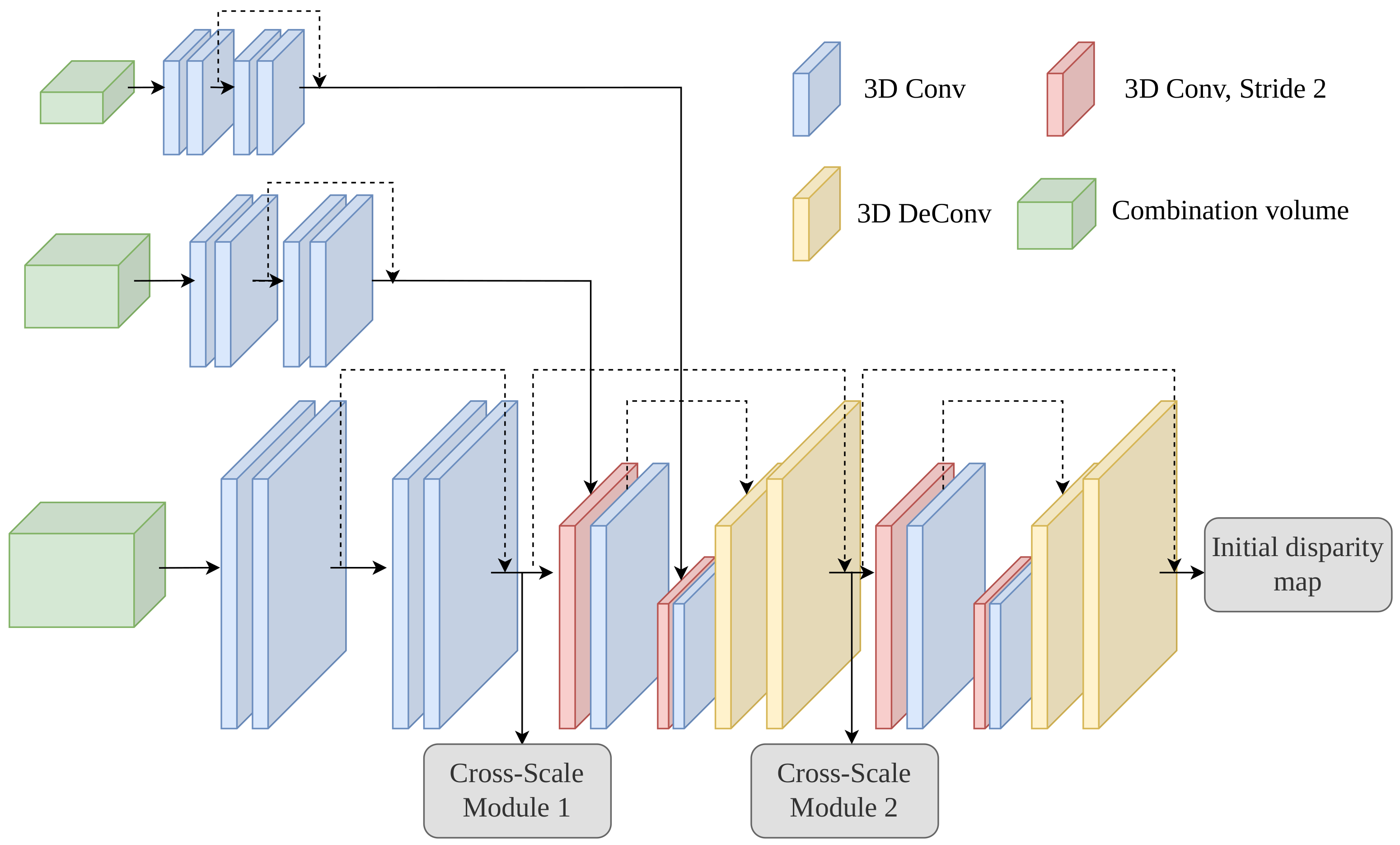
2.1. The Architecture of the Proposed Network

The overall architecture of the proposed network is shown in Figure 3. Given a rectified remote sensing image pair $I_l$ and $I_r$, we first employ a siamese UNet-like [37,38] module to extract multi-scale features, which shares an encoder-decoder architecture with skip connections between multi-scale feature maps (as shown in Figure 4). The encoder is composed of five residual blocks followed by a SPP module to better incorporate multi-scale context information. The encoder module is similar to HSMNet [37] and CFNet [30] and which is proven to be efficient and contains various context information. Moreover, the decoder upsamples the hierarchical feature maps and concatenates them with the feature maps from skip links of the encoder. Then, the extracted multi-scale features are fed into multi-scale group-wise cost volume construction.

Different from one-stage cost aggregation methods [23,24,25], multi-stage cost aggregation methods [28,29,30] are proven to be more effective, which can reduce the computational complexity and time cost by progressively refining the disparity estimation. We divide multi-scale feature maps into fused and cascade cost volumes to predict multi-resolution disparity, respectively, and we fuse multi-scale cost aggregation results to capture low and high resolution information. In addition, we build a multi-scale confidence prediction module to regularize cost distributions and leverage the learned confidence map to generate the next stage’s disparity search range progressively. The training loss functions employed in our method are the stereo focal loss [31] and smoothL1 loss [24,25], which are used to regularize cost distribution and disparity, respectively. The details of the aforementioned modules will be discussed in the following sections.

2.2. Fused Cost Volume of the Coarsest-Scale Feature

In the cascade multi-scale cost aggregation frameworks, generating low-resolution initial disparity maps is indispensable. Different from the existing methods [29,39] which do not use low-resolution feature maps, CFNet fuses three lowest resolution feature maps to generate a more accurate initial disparity map in an encode-decoder process. Noticing the effectiveness of this module, we adopt the same cost volume construction in CFNet, which uses both concatenated and group-wise correlation [26] feature maps to generate low-resolution cost volume. The detail of the combined volume is given as:

$$\begin{array}{cc}\hfill C_{concat}^i(d^i,x,y,f)& =F_l^i(x,y)\oplus F_r^i(x-d^i,y)\hfill \\ \hfill C_{gwc}^i(d^i,x,y,f)& =\frac{1}{N_c^i/N_g}\langle F_l^i(x,y),F_r^i(x-d^i,y)\rangle \hfill \\ \hfill C_{combine}^i& =C_{concat}^i\oplus C_{gwc}^i\hfill \end{array}$$

(1)

where $F_l^i$ and $F_r^i$ are the extracted feature maps at scale i and $N_c$ represents the number of feature channel. $N_g$ is the group size of correlation. $\langle ,\rangle$ denotes the inner product and ⊕ is the feature concatenation.

By densely sampling the whole disparity range in low resolution, the hypothesis plane interval equals to 1, by which we can efficiently generate the initial cost volume with size $H/2^i\times W/2^i\times D_{max}/2^i\times F$. Then, the improved encoder-decoder architecture with 3D hourglass aggregation module is used to fuse the three lowest cost volumes. As shown in Figure 5, specifically, the combination volumes from 1/32, 1/16 scale, firstly employed four 3D convolution layers and skip connections, respectively, are concatenated into the scale 1/8. In addition, the 3D hourglass network is implemented to further aggregate the fusion cost volume, and the intermediate outputs are used for the following cross-scale cost aggregation and the confidence-aware algorithm can be employed based on the final output of this scale.

As shown in Figure 1, due to the various disparity ranges in remote sensing images, the cost volume and its disparity regression range need to be reset to accommodate remote sensing images. According to the disparity regression algorithm [23], the probability of each disparity d is calculated from the predicted cost $c_d$ via the softmax operation. Then, the continuous disparity maps $\hat{d}$ can be calculated by the weighted sum of d. In this paper, we reconstruct the three initial coarsest-scale cost volumes with the range of $[-D_{max}^i,D_{max}^i]$ same to the corresponding disparity regression range. As shown in Figure 6, the coarsest cost volumes have size of $[2\times F^i\times H^i\times W^i]$, which are suitable for the characteristics of remote sensing images, where $D_{max}^i$ is the max disparity at scale i and $F^i,H^i,W^i$ denote the dimension size of feature, height, and width at scale i, respectively. Thus, the three coarsest-scale predicted disparity maps $\widehat{d^i}$ can be calculated as follows,

$$\widehat{d^i}=\sum _{d=-D_{max}^i}^{D_{max}^i}d\times softmax(-c_d^i).$$

(2)

where $softmax$ means the softmax operation, and $c_d^i$ denotes the estimated cost volume at scale i. $softmax(-c_d^i)$ is the discrete disparity probability distribution.

2.3. Confidence-Based Unimodal Distribution Regularization

Aiming at generating the next stage disparity search range based on the initial fusion disparity estimation, existing methods [28] make a straightforward, uniformly sampling with a predefined range. However, such a method cannot adaptively adjust pixel-wise property. The pixels in challenging areas should empirically expand their search ranges. To tackle this problem, refs. [30,31] propose a variance-based disparity range search algorithm and a pixel-wise confidence map to adaptively quantify the various search ranges. The degree of multimodal distribution is highly correlated to the probability of prediction error. Different from the previous works, we adopt the learnable confidence estimation networks [31] to embed in the multi-scale variance-based disparity refinement framework. The multi-scale confidence estimation network and cascade disparity refinement framework are presented in the following subsection.

Cost volume usually reflects the similarities between corresponding pixel pairs, where the truly matched pixel should have the lowest cost or the highest similarity [31]. This hypothesis requires the cost distribution is unimodal peaked at the true disparity and increases with the distance to the true position. The unimodal distribution truth is defined as:

$$\begin{array}{cc}\hfill P\left(d\right)& =softmax(-\frac{\left|d-d^{gt}\right|}{\sigma })\hfill \\ \hfill & =\frac{exp(-c_d^{gt})}{{\sum }_{d^{\prime }=-D_{max}^i}^{D_{max}^i}exp(-c_{d^{\prime }}^{gt})}\hfill \end{array}$$

(3)

where $c_d^{gt}=\frac{\left|d-d^{gt}\right|}{\sigma },\sigma >0$ is the variance that controls the sharpness of the peak around the true disparity. It is clear that pixels across different challenging areas should have different cost distribution. For example, a pixel at a robust corner usually has a sharp peak, while pixels in textureless regions may have flat distribution. Consequently, we add a confidence estimation network to adaptively predict the $\sigma$ for each pixel. In the meantime, the predicted confidence maps are used to compute the next stage disparity search range and employ the multi-scale stereo focal loss combined with $P\left(d\right)$.

The confidence estimation network takes the predicted cost volume as input and uses a few layers to predict a confidence map for each pixel. The network consists of a $3\times 3$ convolutional layer followed by BN and ReLU, and another $1\times 1$ convolutional layer followed by sigmoid activation, after which we can predict a confidence map $f\in {[0,1]}^{H^i\times W^i}$. The larger confidence value refers to a more robust correspondence. Then, the $\sigma$ of cost distribution truth is calculated as:

$${\sigma }^i=\alpha (1-f^i)+\beta$$

(4)

where $\alpha >0$ is the scale factor and $\beta >0$ is the lower bound for $\sigma$ and avoids numerical error of zero-dividing. Accordingly, the cost distribution truth in Equation (3) should be modified.

2.4. Cascade Cost Volume for Disparity Refinement

Given the predicted confidence maps, the variance value ${\sigma }^i$ can be computed through Equation (4). Therefore, it is reasonable to implement the confidence-aware variance to evaluate the disparity search range of the next stage, where lower confidence value corresponds to a wider search space to correct the wrong estimation [30]. Thus, the next stage’s disparity search range can be computed as:

$$\begin{array}{cc}\hfill d_{max}^{i-1}& =\delta (\widehat{d^i}+(s^i+1){\sigma }^i+{\epsilon }^i)\hfill \\ \hfill d_{min}^{i-1}& =\delta (\widehat{d^i}-(s^i+1){\sigma }^i-{\epsilon }^i)\hfill \\ \hfill -D_{max}^i& \le d_{max}^i,d_{min}^i\le D_{max}^i\hfill \end{array}$$

(5)

where $\delta$ means bilinear interpretation. $s^i, {\epsilon }^i$ are two learnable hyperparameters, which are initialized as 0. The two learnable parameters are proven to be more robust [30] than human-selected parameters. Finally, the next stage’s disparity search range can be uniformly sampled as:

$$\begin{array}{cc}\hfill d^{i-1}& =d_{min}^{i-1}+n(d_{max}^{i-1}-d_{min}^{i-1})/(N^{i-1}-1)\hfill \\ \hfill n& \in 0,1,2\dots N^{i-1}-1\hfill \end{array}$$

(6)

where $N^{i-1}$ is the number of disparity hypothesis planes at stage $i-1$. Then, the cost volume of the next stage with size $\frac{H}{2^{i-1}}\times \frac{W}{2^{i-1}}\times N^{i-1}\times F$ is generated.

After that, we employ a similar 3D hourglass cost aggregation module in $1/8$ scale to predict the refined disparity map. Thus, the coarse-to-fine cascade disparity estimation framework is built by progressively narrowing down the disparity search range.

2.5. Cross-Scale Cost Aggregation

The cross-scale interaction in stereo matching, not only introduced in the traditional algorithm [36] but the learning-based methods [22,40], is observed as beneficial to aggregate multi-scale feature information. In addition, the cross interaction modules in HRNet [41] are proposed for learning sufficient feature representations for human pose estimation. With the observation application on remote sensing images that the recent popular methods pay more attention to large-scale objects, as shown in Figure 2, we add the cross-scale interaction module to further aggregate rich cost information in our cascade framework.

With the analyses in [22,36], we add a similar combination manner in HRNet, which adaptively fuse the cost volume results performed in different scales. Specifically, the cross-scale combination is:

$$\begin{array}{cc}\hfill \widehat{C^i}& =\sum _{k=1}^i{f}_k\left(\widetilde{C^k}\right)\hfill \\ \hfill f_k& =\{\begin{array}{cc}\tau & ,k=i\\ \delta (.)\oplus 1\times 1conv& ,k>i\end{array}\hfill \end{array}$$

(7)

where $\widehat{C^i}$ is the cost volume after cross-scale cost aggregation, while $\widetilde{C^k}$ is the intermediate outputs of different scales. In addition, $f_k$ defines a general combination function of different-scale cost volume. Specifically in the function $f_k$, the $\tau$ denotes the identify function, while ⊕ means bilinear upsampling ($\delta$) to the consistent resolution i followed by a $1\times 1$ convolution layer.

2.6. Loss Function

Considering the loss function, we first adopt the smooth $L_1$ loss to supervise the multi-scale estimated disparity map and adopt the stereo focal loss, which is proposed in [22], to further regularize the cost distribution based on $P_p\left(d\right), P_{gt}\left(d\right)$. Due to the low sensitivity to outliers compared to $L_1$ loss [42], smooth $L_1$ loss is widely used in object detection and stereo matching, which is given as follows:

$${\mathcal{L}}_{SL}=\frac{1}{N}\sum _{i=1}^{N}smoot{h}_{L1}(d_i-{\widehat{d}}_i),$$

(8)

where

$$smoot{h}_{L1}\left(x\right)=\{\begin{array}{cc}{x}^2/2,\hfill & \mathrm{if}\left|x\right|<1\hfill \\ \left|x\right|-0.5,\hfill & \mathrm{otherwise}\hfill \end{array}$$

where N is the valid disparity in ground truth, d denotes the disparity label, and $\widehat{d}$ is the predicted disparity.

In order to supervise distribution loss between the predict and ground truth and considering the severe sample imbalance problem since one pixel only has one true disparity, the stereo focal loss [31] is proposed to focus on truth disparities, which is inspired by the focal loss [16] designed to solve the sample imbalance problem in object detection [43]. The stereo focal loss is defined as:

$${\mathcal{L}}_{SF}=\frac{1}{N}\sum _{i=1}^N(\sum _{d=-D_{max}^i}^{D_{max}^i}{(1-P\left(d\right))}^{-\gamma }·(-P\left(d\right)·log{P}_{gt}\left(d\right)))$$

(9)

where $\gamma >0$ denotes a focusing parameter, and the loss is deprecated to cross entropy loss when $\gamma =0$, while $\gamma >0$ performs more weights to positive disparities so that the positive disparities only compete with a few negative ones. In conclusion, our final loss functions consist of the aforementioned losses defined as:

$$\mathcal{L}={\lambda }_1{\mathcal{L}}_{SF}+{\lambda }_2{\mathcal{L}}_{SL}$$

(10)

where ${\lambda }_{1,2}$ are two trade-off hyperparameters. In addition, ${\mathcal{L}}_{SF}$ is used to supervise cost volume distribution, while ${\mathcal{L}}_{SL}$ is to supervise disparity maps.

3. Result

In this section, we first introduce the dataset and metrics for evaluation and experimental settings. Then, the experimental results compared to other state-of-the-art networks are presented to evaluate the performance.

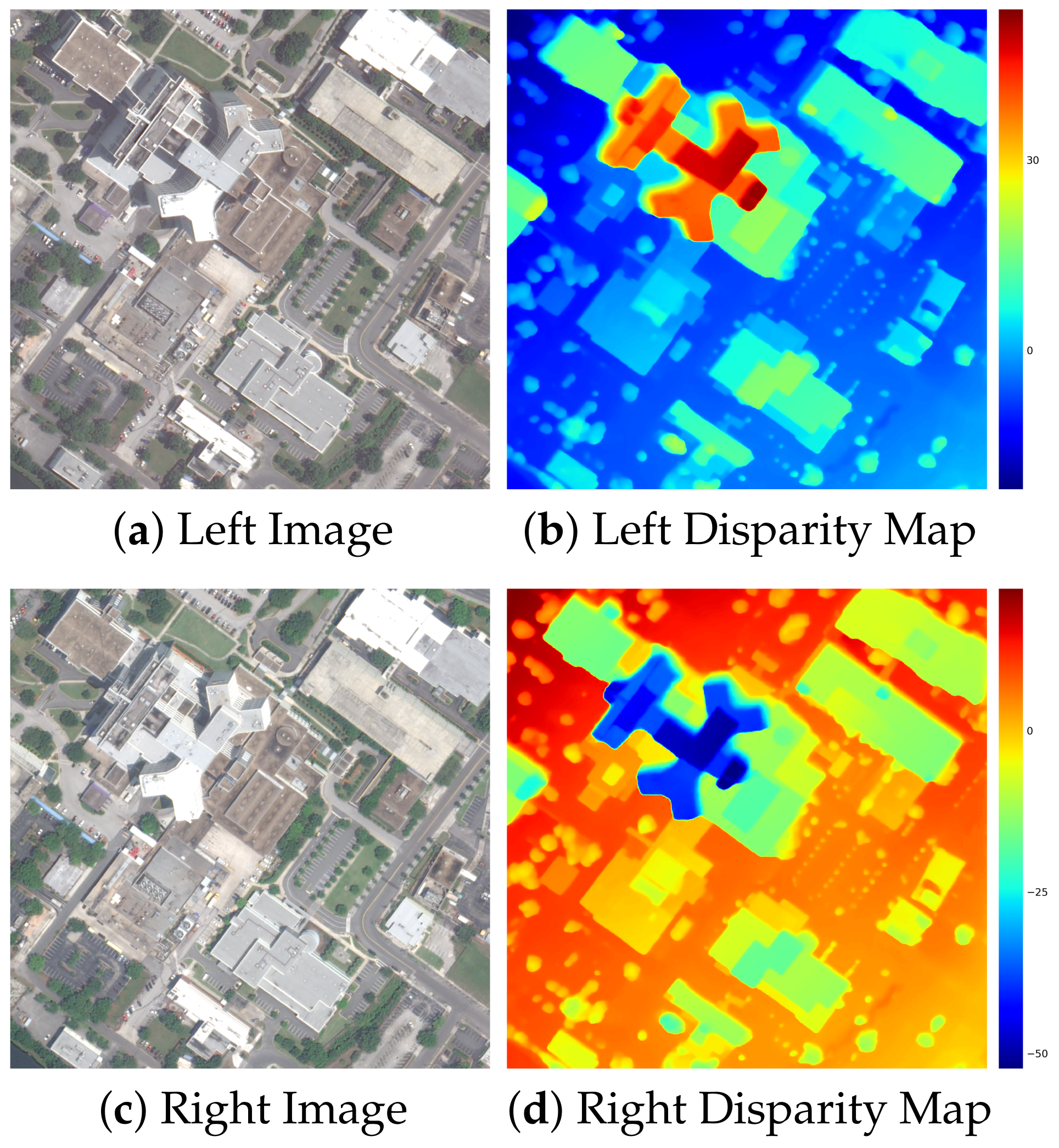
3.1. Datasets and Evaluation Metrics

We conduct extensive experiments on two datasets: SceneFlow and US3D. Both datasets contain positive and negative disparities, and details are listed in

Table 1. The settings of two datasets.

Stereo Pair	Mode	Patch Size	Training Images	Testing Images
SceneFlow	RGB	$960\times 540$	70,908	8740
US3D	RGB	$1024\times 1024$	4292	50

.

(1) The SceneFlow dataset (https://lmb.informatik.uni-freiburg.de/resources/datasets/SceneFlowDatasets.en.html, accessed on 8 February 2022) [20] is a large-scale synthetic dataset including 35,454 positive training and 4370 test images with a resolution of $960\times 540$, so as the negative ones. The RGB images in SceneFlow are rendered into cleanpass and finalpass settings, where cleanpass includes lighting and shading effects. In contrast, the finalpass images also contain motion and defocus blur. We use the whole positive and negative finalpass images to pre-train our network. An example is shown in Figure 7, where there are similar-scale objects in the foreground.

(2) The US3D dataset (https://ieee-dataport.org/open-access/data-fusion-contest-2019-dfc2019, accessed on 8 February 2022) is the track2 data of the 2019 IEEE Data Fusion Contest [34,35]. The stereo pairs in this dataset are from 69 VHR WorldView-3 multi-view remote sensing images, which are acquired from 2014 to 2016 over Jacksonville and Omaha in the United States. The stereo pairs in this dataset are geographically non-overlapped with the rectified size of $1024\times 1024$. The whole dataset has 4292 and 50 stereo pairs for training and testing, which contain various landscapes such as residential buildings, skyscrapers, woods, and rivers. An example is shown in Figure 8, which contains more complex multi-scale objects compared with SceneFlow.

In order to evaluate our proposed network, two quantitative metrics, the average endpoint error in pixels (EPE) and the fraction of erroneous pixels (D1), are used to assess the performance. D1 is robust to outliers with large disparity errors, while EPE measures errors to sub-pixel level.

3.2. Implementation Details

We use PyTorch to implement our network and employ the Adam optimizer with ${\beta }_1=0.9$, ${\beta }_2=0.999$ to train the whole network in an end-to-end way. The input size of images is set to $512\times 512$. The asymmetric chromatic augmentation and asymmetric occlusion [30,37] are used for data augmentation.

We implement a two-stage strategy to train our network. Specifically, we first pre-train our model in the SceneFlow dataset from scratch for 20 epochs, and then finetune our pre-trained model on US3D dataset for 300 epochs. In the whole training process, the initial learning rate is set to 0.001 and is downscaled by 10 after epoch 200. We normalize the pixel to $[0,1]$ to decrease the radiometric influence in remote sensing images. Every experiment is conducted on 2 NVIDIA Titan-RTX GPUs with every 8 mini-batch.

The disparity regression range is set to $[-128,128]$. Since the variance ${\theta }_p$ reflects the shape of unimodal distribution, it is bounded in $[\alpha ,\alpha +\beta ]$. For the best performance of disparity estimation for remote sensing images, we set the $\alpha =1.0, \beta =1.0$, respectively. Then, the parameter $\gamma$ in stereo focal loss is set to 5.0 to balance positive and negative disparity samples. As for the three weighted parameters in smooth $L_1$ loss, we follow the settings in previous stacked hourglass networks [24,25,30,32], and set $0.5, 0.7, 1.0$ for the three intermediate outputs respectively. In our final loss function, the ${\lambda }_1, {\lambda }_2$ are set to $1.0, 0.8$, respectively, to balance the three training losses.

3.3. Comparisons with Other Stereo Methods

To further evaluate the effectiveness of the proposed network, we conduct the comparative experiments with state-of-the-art stereo matching networks, including CasStereo and CFNet which are also based on cascade disparity refinement frameworks, AANet proposed for real-time stereo matching, PSMNet which is a typical stereo matching network, and AcfNet improving PSMNet with cost regularization. The end-point error (EPE) and 3-pixel error (D1) are used to assess the quantitative performance, where EPE is the mean disparity error in pixels and 3-pixel error is the average percentage of pixel whose EPE is bigger than 3 pixels. In order to illustrate the visual results of the improvements, we compute the pixel-wise error map to evaluate the prediction error; cold colors in the error map denote small prediction errors, while warm colors denote large prediction errors. The quantitative result is shown in

Table 2. The quantitative results of different network.

Networks	SceneFlow		US3D
	EPE (Pixel)	D1 (%)	EPE (Pixel)	D1 (%)
PSMNet	1.20	4.69	1.82	14.17
AANet	1.13	4.51	1.91	14.33
AcfNet	1.15	4.69	1.73	12.51
CasStereo	1.10	4.50	1.85	13.93
CFNet	1.02	4.42	1.63	12.72
Our	0.95	4.39	1.41	10.28

, which reflects the performance of networks trained on both the SceneFlow and US3D test datasets. Obviously, our network outperforms them on remote sensing images pretrained on SceneFlow. That is mainly because the proposed network holds the ability to estimate accurate disparities for multi-scale objects in remote sensing images. Subsequently, we illustrate some visual results of US3D samples with two multi-stage cascade networks to further show the improvements on multi-scale objects.

Herein, Figure 9 illustrates the visual performance of disparity estimation between our method with different algorithms. There are multiple landscapes in multi-scale scenarios. Obviously, from the disparity map and error map, our method shows many improvements in such multi-scale disparity estimation, while the other performs badly in large-scale or small-scale disparity estimation. This proves the effectiveness of our proposed multi-scale module. It is noteworthy that the insight of cascade disparity refinement framework has also been investigated in CasStereo and CFNet. CasStereo predicts an initial disparity estimation by constructing higher-resolution sparse cost volume and progressively, uniformly samples a pre-defined range to generate the next stage disparity search range. In addition, CFNet argues that the fusion of small resolution cost volume can generate a more accurate initial disparity map than higher-resolution sparse cost volume. However, from the quantitative and visual illustration in implementing the aforementioned methods on VHR remote sensing images, CasStereo cannot perform well on such larger-scale disparity estimation since the initial high-resolution sparse cost volume cannot catch a sufficient large context with the first stage’s network. In contrast, CFNet performs well in large-scale disparity by losing the disparity accuracy in such a small scale, which proves the effectiveness of initial cost volume fusion. The large-scale disparity information can be well initialized based on such small resolution cost volume. Nevertheless, more complex scenarios make such cascade disparity refinement frameworks perform worse without multi-scale information interaction. Consequently, our method leverages sufficient multi-scale cost volume interaction to tackle this problem in VHR remote sensing images. From the illustration from Figure 9, our method with cross-scale cost volume interaction performs best both in the large and small scale of disparity estimation.

4. Discussion

In this section, we conduct ablation experiments for evaluating the effectiveness of each module in our proposed network.

4.1. Analysis of the Variance-Based Methods

Variance estimation is an important component of the disparity refinement framework, which can automatically adjust the flatness of the unimodal distribution according to the matching uncertainty. The variance of unimodal distribution can be uniformly set for all pixels, while CFNet proposes adaptive uncertainty maps based on the pixel-wise disparity candidates. Different from these methods, we leverage a learnable cost refine module to compute confidence maps. For comparison, we respectively implement the uniform setting, uncertainty-based method in CFNet, and our confidence-based module on US3D dataset.

Figure 10 shows several pixel-wise results from SceneFlow and US3D, where the confidence maps show that the synthetic SceneFlow has many simple structures, while there are more complex scenarios in VHR remote sensing images. As expected in such challenging regions: occlusions, thin structures, textureless patterns; the confidence map in our method provides high variances to flatten the corresponding disparity cost distributions, which can balance the cost aggregation for different pixels.

Table 3. The quantitative results of different variance-based methods.

Networks	US3D
	EPE (Pixel)	D1 (%)
Our(uniform)	1.62	12.13
Our(with uncertainty)	1.45	10.59
Our(with learned confidence)	1.41	10.28

shows the results of implementing different variance-based methods. The results demonstrate the effectiveness of adaptive variance estimation. Comparing with the uncertainty-based method in CFNet, our learnable confidence-based method gives more improvements.

4.2. Analysis of the Cross-Scale Interaction Module

To further evaluate the effectiveness of the cross-scale cost volume aggregation module, we add such modules in CasStereo and CFNet which are called CasStereo-c and CFNet-c, respectively. The quantitative results are listed in

Table 4. The quantitative results of re-implemented methods with cross-scale module.

Networks	US3D
	EPE (Pixel)	D1 (%)
CasStereo-c	1.52	11.63
CFNet-c	1.47	10.41
Our	1.41	10.28

. Comparing with the results from Table 2, equipped with our proposed cross-scale interaction module, CasStereo-c and CFNet-c both improve a lot in terms of EPE and D1. Figure 11 shows the visual results of disparity estimation of re-implemented CasStereo-c, CFNet-c and our method. As we expect, the disparity maps and corresponding error maps both illustrate the significant improvements in multi-scale regions, which prove the effectiveness of the proposed cross-scale interaction module in VHR remote sensing scenarios.

4.3. Analysis of the Loss Settings

In our proposed network, the stereo focal loss and smooth L1 loss are employed to supervise cost volume distribution and disparity estimation map, respectively. First, to evaluate the effectiveness of stereo focal loss applied in remote sensing images, we equip our method with stereo focal loss, cross entropy loss, and none.

Table 5. The quantitative results of different loss function.

Networks	US3D
	EPE (Pixel)	D1 (%)
Our + None	1.47	10.41
Our + Cross Entropy Loss	1.43	10.41
Our + Stereo Focal Loss	1.41	10.28

illustrates the results. It is obvious that the stereo focal loss performs better than cross entropy loss, which demonstrates the effectiveness of balancing weight from positive and negative disparities.

In order to find the optimal ${\lambda }_1$, ${\lambda }_2$ setting in our final loss function, we implement different experimental settings of ${\lambda }_1$, and ${\lambda }_2$ between $[0,1]$. As shown in

Table 6. The quantitative results of different parameters in final loss.

Loss Weight		EPE (Pixel)
${\mathbf{\lambda }}_{\mathbf{1}}$	${\mathbf{\lambda }}_{\mathbf{2}}$
1.0	0.0	1.45
1.0	0.1	1.45
1.0	0.3	1.44
1.0	0.5	1.43
1.0	0.8	1.41
1.0	1.0	1.42

, the weight setting of 0.8 for stereo focal loss and 1.0 for smooth $L_1$ yields the best performance.

5. Conclusions

In this paper, we develop a novel confidence-aware unimodal cascade and fusion pyramid network to improve the disparity estimation for multi-scale objects in VHR satellite images. We first use the fused cost volume from the coarsest scale to generate an initial disparity map, and then construct the unimodal cost distributions by a learnable confidence prediction network, which are able to narrow down the next-stage disparity search range. Moreover, we design a cross-scale interaction aggregation module to leverage multi-scale information. In the whole training process, both smooth-L1 loss and stereo focal loss are applied to regularize the disparity map and unimodal cost distribution, respectively. Our network shows a strong ability to handle multi-scale disparity estimation. Experiment results show that our network performs well compared to two state-of-the-art stereo matching networks with higher precision.

Nowadays, with the gradual growth of data volume of remote sensing images, it is difficult to annotate enough ground truth for a deep learning model to train. Thus, the deep model should perform well on unseen scenarios; however, our network cannot generate satisfactory results for the domain adaptation task of stereo matching. Therefore, in order to make our proposed network work for other datasets without ground truth, we plan to try it in self-supervised ways and extract domain-invariant features.

References

1. Niu, C.; Zhang, J.; Wang, Q.; Liang, J. Weakly Supervised Semantic Segmentation for Joint Key Local Structure Localization and Classification of Aurora Image. IEEE Trans. Geosci. Remote Sens. 2018, 56, 7133–7146. [Google Scholar] [CrossRef]
2. Chen, H.; Lin, M.; Zhang, H.; Yang, G.; Xia, G.S.; Zheng, X.; Zhang, L. Multi-Level Fusion of the Multi-Receptive Fields Contextual Networks and Disparity Network for Pairwise Semantic Stereo. In Proceedings of the International Geoscience and Remote Sensing Symposium, Yokohama, Japan, 28 July–2 August 2019. [Google Scholar]
3. Chen, C.; Seff, A.; Kornhauser, A.L.; Xiao, J. DeepDriving: Learning Affordance for Direct Perception in Autonomous Driving. In Proceedings of the International Conference on Computer Vision, Santiago, Chile, 7–13 December 2015. [Google Scholar]
4. Schmid, K.; Tomic, T.; Ruess, F.; Hirschmüller, H.; Suppa, M. Stereo vision based indoor/outdoor navigation for flying robots. In Proceedings of the 2013 IEEE/RSJ International Conference on Intelligent Robots and Systems, Tokyo, Japan, 3–7 November 2013. [Google Scholar]
5. Engel, J.; Stückler, J.; Cremers, D. Large-scale direct SLAM with stereo cameras. In Proceedings of the Intelligent Robots and Systems, Hamburg, Germany, 28 September–2 October 2015. [Google Scholar]
6. Luo, C.; Yu, L.; Yang, E.; Zhou, H.; Ren, P. A benchmark image dataset for industrial tools. Pattern Recognit. Lett. 2019, 125, 341–348. [Google Scholar] [CrossRef]
7. Scharstein, D.; Szeliski, R. A taxonomy and evaluation of dense two-frame stereo correspondence algorithms. Int. J. Comput. Vis. 2002, 47, 7–42. [Google Scholar] [CrossRef]
8. Sun, J.; Shum, H.Y.; Zheng, N. Stereo Matching Using Belief Propagation. In Proceedings of the European Conference on Computer Vision, Copenhagen, Denmark, 28–31 May 2002. [Google Scholar]
9. Kolmogorov, V.; Zabih, R. Computing visual correspondence with occlusions using graph cuts. In Proceedings of the International Conference on Computer Vision, Vancouver, BC, Canada, 7–14 July 2001. [Google Scholar]
10. Yoon, K.J.; Kweon, I.S. Adaptive support-weight approach for correspondence search. IEEE Trans. Pattern Anal. Mach. Intell. 2006, 28, 650–656. [Google Scholar] [CrossRef] [PubMed]
11. Rhemann, C.; Hosni, A.; Bleyer, M.; Rother, C.; Gelautz, M. Fast cost-volume filtering for visual correspondence and beyond. In Proceedings of the Computer Vision and Pattern Recognition, Colorado Springs, CO, USA, 20–25 June 2011. [Google Scholar]
12. Min, D.; Lu, J.; Do, M.N. A revisit to cost aggregation in stereo matching: How far can we reduce its computational redundancy? In Proceedings of the International Conference on Computer Vision, Barcelona, Spain, 6–13 November 2011. [Google Scholar]
13. Hermann, S.; Klette, R.; Destefanis, E. Inclusion of a second-order prior into semi-global matching. In Pacific-Rim Symposium on Image and Video Technology; Springer: Berlin/Heidelberg, Germany, 2009; pp. 633–644. [Google Scholar]
14. Zhu, K.; d’Angelo, P.; Butenuth, M.; Angelo, P.; Butenuth, M. A performance study on different stereo matching costs using airborne image sequences and satellite images. In Lecture Notes in Computer Science, Proceedings of the ISPRS Conference on Photogrammetric Image Analysis, Munich, Germany, 5–7 October 2011; Springer: Berlin/Heidelberg, Germany, 2011; pp. 159–170. [Google Scholar]
15. Hirschmüller, H. Stereo processing by semiglobal matching and mutual information. IEEE Trans. Pattern Anal. Mach. Intell. 2008, 30, 328–341. [Google Scholar] [CrossRef] [PubMed]
16. Žbontar, J.; LeCun, Y. Stereo matching by training a convolutional neural network to compare image patches. J. Mach. Learn. Res. 2016, 17, 2287–2318. [Google Scholar]
17. Luo, W.; Schwing, A.G.; Urtasun, R. Efficient deep learning for stereo matching. In Proceedings of the IEEE Conference on Computer Vision and Pattern Recognition, Las Vegas, NV, USA, 27–30 June 2016; pp. 5695–5703. [Google Scholar]
18. Guney, F.; Geiger, A. Displets: Resolving stereo ambiguities using object knowledge. In Proceedings of the IEEE Conference on Computer Vision and Pattern Recognition, Boston, MA, USA, 7–12 June 2015; pp. 4165–4175. [Google Scholar]
19. Seki, A.; Pollefeys, M. Sgm-nets: Semi-global matching with neural networks. In Proceedings of the IEEE Conference on Computer Vision and Pattern Recognition, Honolulu, HI, USA, 21–26 July 2017; pp. 231–240. [Google Scholar]
20. Mayer, N.; Ilg, E.; Hausser, P.; Fischer, P.; Cremers, D.; Dosovitskiy, A.; Brox, T. A large dataset to train convolutional networks for disparity, optical flow, and scene flow estimation. In Proceedings of the IEEE Conference on Computer Vision and Pattern Recognition, Las Vegas, NV, USA, 27–30 June 2016; pp. 4040–4048. [Google Scholar]
21. Tonioni, A.; Tosi, F.; Poggi, M.; Mattoccia, S.; Stefano, L.D. Real-Time Self-Adaptive Deep Stereo. In Proceedings of the Computer Vision and Pattern Recognition, Long Beach, CA, USA, 16–20 June 2019. [Google Scholar]
22. Xu, H.; Zhang, J. AANet: Adaptive Aggregation Network for Efficient Stereo Matching. In Proceedings of the Computer Vision and Pattern Recognition, Seattle, WA, USA, 13–19 June 2020. [Google Scholar]
23. Kendall, A.; Martirosyan, H.; Dasgupta, S.; Henry, P. End-to-End Learning of Geometry and Context for Deep Stereo Regression. In Proceedings of the International Conference on Computer Vision, Venice, Italy, 22–29 October 2017. [Google Scholar]
24. Chang, J.R.; Chen, Y.S. Pyramid Stereo Matching Network. In Proceedings of the Computer Vision and Pattern Recognition, Salt Lake City, UT, USA, 18–23 June 2018. [Google Scholar]
25. Zhang, F.; Prisacariu, V.A.; Yang, R.; Torr, P.H.S. GA-Net: Guided Aggregation Net for End-To-End Stereo Matching. In Proceedings of the Computer Vision and Pattern Recognition, Long Beach, CA, USA, 16–20 June 2019. [Google Scholar]
26. Guo, X.; Kai, Y.; Wukui, Y.; Wang, X.; Li, H. Group-Wise Correlation Stereo Network. In Proceedings of the Computer Vision and Pattern Recognition, Long Beach, CA, USA, 16–20 June 2019. [Google Scholar]
27. Sun, D.; Yang, X.; Liu, M.Y.; Kautz, J. PWC-Net: CNNs for Optical Flow Using Pyramid, Warping, and Cost Volume. In Proceedings of the Computer Vision and Pattern Recognition, Salt Lake City, UT, USA, 18–22 June 2018. [Google Scholar]
28. Gu, X.; Fan, Z.; Zhu, S.; Dai, Z.; Tan, F.; Tan, P. Cascade Cost Volume for High-Resolution Multi-View Stereo and Stereo Matching. In Proceedings of the Computer Vision and Pattern Recognition, Seattle, WA, USA, 13–19 June 2020. [Google Scholar]
29. Cheng, S.; Xu, Z.; Zhu, S.; Li, Z.; Li, L.E.; Ramamoorthi, R.; Su, H. Deep Stereo Using Adaptive Thin Volume Representation With Uncertainty Awareness. In Proceedings of the Computer Vision and Pattern Recognition, Seattle, WA, USA, 13–19 June 2020. [Google Scholar]
30. Shen, Z.; Dai, Y.; Rao, Z. CFNet: Cascade and Fused Cost Volume for Robust Stereo Matching. In Proceedings of the Computer Vision and Pattern Recognition, Nashville, TN, USA, 20–25 June 2021. [Google Scholar]
31. Zhang, Y.; Chen, Y.; Bai, X.; Yu, S.; Yu, K.; Li, Z.; Yang, K. Adaptive Unimodal Cost Volume Filtering for Deep Stereo Matching. In Proceedings of the National Conference on Artificial Intelligence, New York, NY, USA, 7–12 February 2020. [Google Scholar]
32. Tao, R.; Xiang, Y.; You, H. An Edge-Sense Bidirectional Pyramid Network for Stereo Matching of VHR Remote Sensing Images. Remote Sens. 2020, 12, 4025. [Google Scholar] [CrossRef]
33. Osco, L.P.; Junior, J.M.; Ramos, A.P.M.; de Castro Jorge, L.A.; Fatholahi, S.N.; de Andrade Silva, J.; Matsubara, E.T.; Pistori, H.; Gonçalves, W.N.; Li, J. A Review on Deep Learning in UAV Remote Sensing. arXiv 2021, arXiv:2101.10861. [Google Scholar] [CrossRef]
34. Saux, B.L.; Yokoya, N.; Hänsch, R.; Brown, M.; Hager, G. 2019 Data Fusion Contest [Technical Committees]. IEEE Geosci. Remote Sens. Mag. 2019, 7, 103–105. [Google Scholar] [CrossRef]
35. Bosch, M.; Foster, K.; Christie, G.; Wang, S.; Hager, G.D.; Brown, M. Semantic Stereo for Incidental Satellite Images. In Proceedings of the Workshop on Applications of Computer Vision, Waikoloa Village, HI, USA, 7–11 January 2019. [Google Scholar]
36. Zhang, K.; Fang, Y.; Min, D.; Sun, L.; Yang, S.; Yan, S.; Tian, Q. Cross-Scale Cost Aggregation for Stereo Matching. In Proceedings of the Computer Vision and Pattern Recognition, Columbus, OH, USA, 23–28 June 2014. [Google Scholar]
37. Yang, G.; Manela, J.; Happold, M.; Ramanan, D. Hierarchical Deep Stereo Matching on High-Resolution Images. In Proceedings of the Computer Vision and Pattern Recognition, Long Beach, CA, USA, 16–20 June 2019. [Google Scholar]
38. Ronneberger, O.; Fischer, P.; Brox, T. U-Net: Convolutional Networks for Biomedical Image Segmentation. In Proceedings of the Medical Image Computing and Computer-Assisted Intervention, Munich, Germany, 5–9 October 2015. [Google Scholar]
39. Yang, J.; Mao, W.; Alvarez, J.M.; Liu, M. Cost Volume Pyramid Based Depth Inference for Multi-View Stereo. In Proceedings of the Computer Vision and Pattern Recognition, Seattle, WA, USA, 13–19 June 2020. [Google Scholar]
40. Xu, Q.; Tao, W. Multi-Scale Geometric Consistency Guided Multi-View Stereo. In Proceedings of the Computer Vision and Pattern Recognition, Long Beach, CA, USA, 16–20 June 2019. [Google Scholar]
41. Sun, K.; Xiao, B.; Liu, D.; Wang, J. Deep High-Resolution Representation Learning for Human Pose Estimation. In Proceedings of the Computer Vision and Pattern Recognition, Long Beach, CA, USA, 16–20 June 2019. [Google Scholar]
42. Girshick, R. Fast r-cnn. In Proceedings of the International Conference on Computer Vision, Santiago, Chile, 7–13 December 2015; pp. 1440–1448. [Google Scholar]
43. Lin, T.Y.; Goyal, P.; Girshick, R.; He, K.; Dollár, P. Focal Loss for Dense Object Detection. In Proceedings of the International Conference on Computer Vision, Venice, Italy, 22–29 October 2017. [Google Scholar]
Figure 1. The disparity range in VHR remote sensing dataset US3D, where every scatter represents one ground truth DSP and the D m a x ,   D m i n denote the maximum and minimum disparity value, respectively.
Remotesensing 14 01667 g001
Figure 2. An example on multi-scale disparity estimation of US3D. From left to right: left image, disparity maps predicted by CFNet, the proposed network, and the ground truth.
Remotesensing 14 01667 g002
Figure 3. The architecture of the proposed cascade confidence-aware pyramid network for stereo matching.
Remotesensing 14 01667 g003
Figure 4. The architecture of the siamese feature extraction module.
Remotesensing 14 01667 g004
Figure 5. The architecture of thefused cost module in our network.
Remotesensing 14 01667 g005
Figure 6. The reconstruction of cost volume for remote sensing images.
Remotesensing 14 01667 g006
Figure 7. Visualization of SceneFlow dataset. (a) The left image. (b) The disparity map based on left image. (c) The right image. (d) The disparity map based on right image.
Remotesensing 14 01667 g007
Figure 8. Visualization of US3D dataset. (a) The left image. (b) The disparity map based on left image. (c) The right image. (d) The disparity map based on right image.
Remotesensing 14 01667 g008
Figure 9. The visualization comparison results of different cascade networks on US3D dataset. For each example, the first row shows the disparity map, and the second row shows the error map. Cold colors in the error map denote small prediction errors, while warm colors denote large prediction errors.
Remotesensing 14 01667 g009aRemotesensing 14 01667 g009b
Figure 10. The visualization results of confidence map for SceneFlow and US3D dataset. Cold colors in the error map denote small prediction errors, while warm colors denote large prediction errors. In confidence map, bright colors mean small variances, while dark colors denote high variances.
Remotesensing 14 01667 g010
Figure 11. The visualization comparison results of cascade networks combining with cross-scale interaction module on US3D dataset. For each example, the first row shows the disparity map, and the second row shows the error map. Cold colors in the error map denote small prediction errors, while warm colors denote large prediction errors.
Remotesensing 14 01667 g011aRemotesensing 14 01667 g011b