
Deforestation by Afforestation: Land Use Change in the Coastal Range of Chile


Karlsruhe Institute of Technology (KIT), Institute of Regional Science (IfR), Kaiserstr. 12, 76131 Karlsruhe, Germany
Remote Sens. 2022, 14(7), 1686; https://doi.org/10.3390/rs14071686
Submission received: 10 March 2022
/
Revised: 24 March 2022
/
Accepted: 28 March 2022
/
Published: 31 March 2022
(This article belongs to the Section Forest Remote Sensing)
Abstract
:In southern Chile, an establishment of a plantation-based forest industry occurred early in the industrial era. Forest companies claim that plantations were established on eroded lands. However, the plantation industry is under suspicion to have expanded its activities by clearing near-natural forests since the early 1970s. This paper uses a methodologically complex classification approach from own previously published research to elucidate land use dynamics in southern Chile. It uses spatial data (extended morphological profiles) in addition to spectral data from historical Landsat imagery, which are fusioned by kernel composition and then classified in a multiple classifier system (based on support, import and relevance vector machines). In a large study area (~67,000 km2), land use change is investigated in a narrow time frame (five-year steps from 1975 to 2010) in a two-way (prospective and retrospective) analysis. The results are discussed synoptically with other results on Chile. Two conclusions can be drawn for the coastal range. Near-natural forests have always been felled primarily in favor of the plantation industry. Vice versa, industrial plantations have always been primarily established on sites, that were formerly forest covered. This refutes the claim that Chilean plantations were established primarily to restore eroded lands; also known as badlands. The article further shows that Chile is not an isolated case of deforestation by afforestation, which has occurred in other countries alike. Based on the findings, it raises the question of the extent to which the Chilean example could be replicated in other countries through afforestation by market economy and climate change mitigation.
1. Introduction
Humanity has extensively changed the land cover of large parts of the Earth’s surface [1,2]. Land use changes are closely related not only to climate change [3], changes in Earth’s biogeochemical cycles [4], but also to environmental conflicts [5]. Land use changes related to natural forest conversion are highly debated. While the tree-covered area has increased globally, some regions are experiencing severe regional forest loss, while others are being afforested [1,6]. Afforestation with tree plantations will increase in the future due to market demand for wood products [7] and to create negative emissions [8]. Since planted forest generally can fix CO2, maintain a certain biodiversity and ecosystem services, some authors generally welcome afforestation as a measure that combines climate and environmental protection with economic goals [9], while others are concerned about the consequences for humans [10,11,12] and the environment [13,14,15] in the case of afforestation with commercial monocultures. From these linkages, it is important to understand the relationship between afforestation and land use change using regional empirical examples [16].
Chile is one of the countries that has relied massively on plantation industry at earliest in the industrial age [17]. The first tree plantations were introduced in Chile as early as the late 19th century to stabilize soils that were vulnerable to erosion from agricultural use [18]. Very quickly, however, the Chilean state recognized the strategic potential of the plantation industry sector. On the one hand, there was an increasing market demand for wood-based products, and on the other hand, the plantation industry supported Chile’s industrialization [19]. Two plantation industry laws (1931 and 1974) strongly promoted the expansion of the forestry industry [20]. Particularly controversial is Federal Decree DL 701 (Spanish: Decreto Ley–DL 701) of 1974, which subsidized plantation industry investments by 75% (even 90% during the financial crisis of the 1990s) over an enormously long period (1974 to 1996) [17,21]. Very quickly after the enactment of DL 701, plantation industry companies apparently began not only to replant eroded badlands, but to cut down semi-natural forests in favor of plantations [22]. The process of forest substitution continued until 2008, when after almost 20 years of discussion about this practice, a forest protection law (Ley 20.283) was finally enacted, putting an end to it [23]. Another way to protect forests in the context of forestry is through timber certification. The Chilean forestry industry resisted the international FSC standard for a long time and developed its own certification program, CERTFOR, with limited success [24]. A precise understanding of land use change in Chile is needed to study its social and environmental consequences. Nevertheless, land use change in Chile is still controversially discussed today. Clapp [25] still assumed that most tree plantations were established on already deforested land, e.g., Aguayo et al. [26] see forest expansion as the main factor of land use change. This debate can be clarified above all by area-wide remote sensing surveys.
Land use change in the coastal region of central Chile has already received scientific attention. Using a maximum likelihood classification of a single Landsat scenes at three points in time (1975, 1990, 2000), Echeverria et al. [27] show that forest ecosystems are being replaced by industrial tree plantations. Other studies work on the same dataset or also on single Landsat scenes [26,28,29,30,31,32,33,34]. Heilmayr et al. [35] study a much larger region using 42 Landsat scenes at three time points (1985–1987, 1999–2001, 2009–2011). After a change vector analysis based on a tasseled cap transformation, they perform a maximum likelihood classification. They also demonstrate deforestation in favor of plantations and categorize the Chilean case as a plantation-dominated forest transition in the forest transition theory [36]. Uribe et al. [37] look at a much longer time span than the previous studies. They use aerial imagery (1955–1960), Landsat imagery (1975–1998), and GoogleEarth imagery (from 2014) and perform a visual image interpretation of a 3 × 3 km grid of the entire coastal mountain range. This allows them to show that plantation expansion began before 1960 but was particularly rapid between 1975 and 1998. They also show that 40% of the forests have been replaced by plantations. Nahuelhual et al. [38] use an extended dataset from Echeverria et al. [27], but focus more on an analysis of the drivers of plantation establishment. They show that especially during the early period (1975–1990), tree plantation establishment depended on soil characteristics, slope, proximity to cities, and company ownership as well as the size of properties. They also show that there is a high probability of transition from forest land to plantation land. Miranda et al. [39] summarize the various findings in a review, showing that the greatest forest loss occurred between 1970 and 1990, but that forest loss has continued steadily over the past 40 years, with a total of over 782,000 ha lost (19% of forests in the study area).
Although extensive preliminary work is already available, it leaves some shortcomings. These shortcomings relate to
- The completeness of the overarching approach (perspective on land use change, representation of all plantation types present);
- Temporal design of the study (study period, temporal grid of analysis);
- Spatial design of the study (spatial data resolution);
- Technical design of the study (classification techniques employed).
These shortcomings are briefly addressed:
Firstly, regarding the completeness of the overarching approach, it has to be stated that previous studies have taken a one-sided perspective on land-use change. They have mainly focused on the fact that forest areas have disappeared in favor of plantations. So far, hardly any attention has been paid to the complementary question of on which areas plantations have been established. It is theoretically quite conceivable that almost 100% of the deforested areas were cleared in favor of plantations, but conversely, e.g., 80% of the plantations were established on eroded badlands. To fully understand and, if necessary, politically assess the land-use change process, a two-sided analysis is crucial. Furthermore, most studies, e.g., Uribe et al. [37] only consider Pinus but not Eucalyptus plantations. However, as over 17% of Chilean plantations are planted with Eucalyptus [40] and Eucalyptus plantations have significant environmental impacts [41,42], these should not be ignored. In general, forest plantations are a broad class, which may appear with different tree species, ages and silvicultural treatments. This can bring up issues in the classification procedure. These issues may trigger motivation to reduce the classification to only adult plantations of one particular species. This would the classification procedure, but make the assessment less complete, of course. Secondly, regarding the temporal design of the study, many studies omit important phases of the land use change period. For example, Heilmayr et al. [35] do not consider the dynamic period between 1975 and 1986, and Echeverria et al. [27] do not consider the period after 2000, which is important for today’s forest policies. Furthermore, the temporal grids used by the studies are often very coarse. The studies published so far consider time intervals of 10 to 15 years. However, it must be kept in mind that southern Chile is a very dynamic landscape. The dynamics are explained, for example, by the frequent forest fires [43] and climate change impacts [44], but above all by the rapid and spatially extensive land use change [45]. These dynamics need to be accounted for by short temporal coverage grids [46,47]. For example, 10-to-15-year grids are too long to exclude intermittent land uses. It is quite possible that within 15 years a forested area is first cleared for agriculture, the agriculture is then abandoned, and the area is then planted with plantations. With too rough of a time frame, this situation cannot be distinguished from immediate deforestation for the sake of plantation establishment. A frequent claim in Chile is that plantations are established on abandoned agricultural land to prevent erosion [48]. Therefore, it is crucial to reliably exclude intermittent land uses.
Thirdly, the spatial design of the current state of the art is insufficient. For instance, the study by Uribe et al. [37] considers a very long period, but works on a very coarse grid. A 3 × 3 km grid is 10,000 times coarser than a Landsat pixel. However, as many important deforestation processes are small-scale (e.g., felling of forest remnants during plantation harvesting), sub-processes could be overlooked.
Finally, the technical design can be improved. The classification techniques used are technically rather outdated. Although a better classifier cannot necessarily guarantee more meaningful classifications [49], Braun et al. [50] were able to show that the subtle spectral differences between forests and plantations can be captured much better with more advanced methods.
This study is the first to address the aforementioned limitations. It examines a large study area (67,000 km2) over the entire study period in which major land use change occurred (1975–2010). It works with high resolution data (Landsat data, 60 × 60 m or 30 × 30 m) and with a narrow temporal grid (5 years). This makes it possible to exclude intermittent land uses. It examines land use change from three perspectives, one prospective, one indirect, and one retrospective, in order to fully address the desiderata mentioned earlier.
In order to assess the expansion of the plantation industry completely, not only adult Pinus plantations were considered. Instead, both Eucalyptus and Pinus plantations were classified. Both plantation types were represented by a set of subclasses, which denote the differences in age structure and silvicultural treatment. Afterwards, these subclasses were agglomerated to a single plantation class.
Very high accuracy values are important for this project. Shao and Wu [51] argue that 90% accuracy must be achieved in order to relate land use classifications to the topics of landscape ecology. Braun et al. [50] were able to show that traditional methods—such as maximum likelihood—can detect adult plantations but fail to distinguish younger plantations. These are easily confused with bushlands. However, it is precisely these plantations that are important in order to be able to reliably ascertain whether forests have been replaced by plantations or not. In this research, a complex classification approach was developed, which is used here.
With this approach, the present article pursues an objective that has global significance in the 21st century. Chile is a country where afforestation measures were introduced for the purpose of environmental protection (prevention of soil erosion). Very quickly, however, this goal receded behind economic interests. Several factors led to vast land use change processes. On the one hand, there were wrong economic incentives by massive subsidies [52,53]. On the other hand, there was a lack of environmental policies [54,55]. This land use change inverted the original environmental goal of erosion control [56,57]. Moreover, it triggered further environmental problems [45,58] and exacerbated negative social developments in rural areas [19,59,60]. If one considers that almost 50% of the land designated for afforestation measures as a result of the Paris Agreement is to come from commercial plantations [61] and that many of these areas are located in regions with “weak governance” [8], then it must be feared that the developments observed in Chile will be repeated in other countries.
The first objective of this study is to show how the expansion of the plantation industry in Chile is related to the losses of semi-natural forests. This is to be done in a narrow temporal grid and a large study region. The second goal is to build the analysis based on a (previously developed [50,62,63]) state of the art methodology. Outdated remote sensing techniques could be questioned in terms of their informative value, so that a methodology that is as up-to-date as possible should increase the reliability of the results in the scientific discourse. The third objective is to discuss to what extent Chile exemplifies what developments can be anticipated in the context of afforestation measures in other countries.
The remainder of the paper is organized as follows. Section 2 presents the study site and explains Methods and Materials. The section places particular emphasis on explaining the classification approach in technical terms (cf. also Braun et al. [50,57]) but also in practical terms, and on working out how its results are to be interpreted. Section 3 presents the results. There, the immediate land use results and the results on deforestation and afforestation rates are discussed. However, the emphasis is on the prospective, indirect, and retrospective land use analysis that distinguishes this study from others. Section 4 briefly discusses the results in technical terms, but more importantly relates them to other findings on land use change in Chile. One focus is to relate the findings on Chile to possible consequences of afforestation (due to market demand for wood products or to create negative emissions) in other countries. Section 5 concludes the article and discusses how Chile could be a possible cautionary example for developments in other countries.
2. Materials and Methods
2.1. Study Site
The study site will be characterized in terms of population, physical geography, vegetation, and the industrial forestry model. The study site comprises the entire VII Región del Maule, VIII Región del Biobío, and the XVI Región de Ñuble, which are part of central Chile. The three regions cover an area of about 67,358 km2 and are inhabited by 2.8 million people. The population density of about 41 persons per km2 is one of the highest in the country [61].
The study site extends from 35° to 37°S and thus belongs to the country’s temperate zone. It has a Mediterranean Csb climate (Koeppen-Geiger) with an annual mean temperature around 12 °C and an annual precipitation of about 1300 mm [64]. The area is morphologically determined by the coastal mountains, a mountain range running from NNE to SSW. The central lowlands represent the interior of the country. Towards the east, the Andes form a high mountain region. The basement of the coastal mountain range consists of magmatic and metamorphic rocks from the Palaeozoic, which are overlain by younger (Quaternary and Tertiary) and volcanic material from the Andes [60].
With regard to vegetation, different forest types occur in the study area. In the south of the coastal mountain range and in the Andean slope, deciduous Nothofagus spp. forests dominate. In the north of the study area, on the other hand, sclerophyllous forest (Peumus boldus, Cryptocarya alba etc.) ecosystems dominate. In the central lowlands, the forest is replaced by Acacia caven bushlands. In contrast, Araucaria araucana conifer forests occur at the highest altitudes of the southernmost coastal mountains [62]. The coastal mountain range is one of the most species-rich forest areas in Chile [63].
Regarding the forestry model, the majority of the industrial plantations are based on Pinus radiata and Eucalyptus globulus, and E. nitens species. The plantations are highly managed ecosystems consisting of a single tree species and usually all individuals are of the same age. The subsoil under the trees is sparsely vegetated and inhabited by only a few species, which also applies to the herb layer [64]. Pine and eucalyptus plantations in Chile are fast growing, with P. radiata reaching mean annual increment values MAI m3·ha−1·year−1 between 15 and 34, depending on the soil type [48]. The plantations are cut down after a cycle duration 10 to 25 years by clearing the entire plantation, and at a diameter at breast height (DBH) of 17 to 22 cm [48,65]. Harvest is done in a highly mechanized fashion. Slope plays a marginal role in harvest, and even very steep slopes are harvested. Approximately 75% of the production is exported (mainly to US, Japan, and China), contributing substantially to Chile’s total exports and GDP. The products mainly exported are sawnwood and (chemical) pulpwood, and roundwood plays a minor role [66]. While plantations contribute macroeconomically [48,67], the effects on regional and community welfare remain strongly contested [19,59,68].
2.2. Remote Sensing Datasets
In order to map the entire land use change process in the aftermath of the Federal Decree DL 701 (1974), land use classifications from 1975 to 2010 will be established. As explained at the beginning, a short temporal interval is necessary to achieve the research objectives. The chosen temporal interval is five-year increments. Thus, a total of eight land use maps will be produced (time points tip 1975, 1980, 1985, 1990, 1995, 2000, 2005, and 2010). Data from different Landsat generations were used (Landsat-2/MSS for 1975 and 1980, Landsat-5/TM for 1985, 1990, 1995, 2005, and 2010, Landsat-7/ETM+ for 2000). A total of nine scenes were required to cover the 67,358 km2 of the study area, see Appendix A. It should be noted that a cloud-free image was not available for every study year. Where no suitable scene could be found for a year, scenes from a year earlier or later were added. For instance, the time point 1980 thus partly contains scenes from the year 1979. For instance, in 2000 the following path/row combinations were used: 001/084, 001/085, 001/086, 001/087, 232/085, 233/086, 233/084, 233/085, 232/086 scenes were acquired from USGS EarthExplorer (https://earthexplorer.usgs.gov/, accessed on 12 May 2021, data downloaded between 2009 and 2012). Before classification, the data were atmospherically and topographically corrected. Landsat level 1 scenes were used, which were corrected for atmospheric and topographical effects using the ATCOR3 methodology [69] and the ASTER V.2 digital elevation model [70]. ATCOR3 corrects the influence of bidirectionality (i.e., the influence of differing sun angles and sensor angles towards the surface). Therefore, effects related to different illumination conditions (e.g., slopes pointing towards the sun or away from it) are corrected. This assures that the same land use system does not differ in the spectral data due to shade effects, etc.
2.3. Class Definition, Training Areas, and Class Agglomeration
In the study of Braun [49] it was shown that high accuracy values alone do not necessarily make a classification meaningful. There may even be situations where high accuracy is associated with lower geographical or ecological meaning. The article elaborates that the underlying values and practices of classification need to be made transparent so that classification can actually be used profitably. In particular, the approach emphasizes that three aspects need to be explained regarding training: definition of classes, designation of training areas, and class agglomeration.
The definition of the classes follows the logic of land use classification with a focus on forestry. In Table 1, the main classes defined in this study are presented including their names, abbreviations, and colors in the result figures. The subclasses that were defined and agglomerated to the main classes after classification are given in Appendix B and Appendix C, respectively. The number of training data is provided in Appendix D. The aim of the classification is to reliably characterize changes in the area covered by trees. During fieldwork, (in 2011), a particularly large amount of time was spent in tree-covered landscapes. Less time was spent in agricultural, urban, peri-urban, and low vegetation areas.
For the 2010 time point, initial training areas were identified in situ during the fieldwork. In the field, the different land use systems were visited. A lot of time was spent in the field (over three months in total). A large number of sites were visited. All sites were located in the area delineated as the “study site” in Figure 3. Homogeneous areas representative of the respective land use system were identified. Different tree species and sylvicultural management options were visited in plantations. These initial training areas were digitized in the field with a handheld GPS (Garmin). In addition to the initial training areas defined in the field, some additional areas were designated on the computer after the spectral signatures of the respective land use system could be reliably recognized on the screen using the initial training areas. Of course, this was best possible for the year 2010, which was close to the time of the field work. For the other time points, additional training areas were identified by finding suitable areas for training based on the operator’s experience with their spectral signatures on the screen.
Initially, numerous subclasses were defined, which were then agglomerated (cf. Appendix B and Appendix C). Agglomeration was performed as follows. In many cases, two functionally similar land use types have different spectral signatures. For instance, young Pinus plantations appear with or without herbaceous understory. Hence, two subclasses were defined to represent both conditions. However, since classes are spectrally, but not functionally different, they were agglomerated afterwards. As explained, the overall objective was to capture land use change with respect to forested areas as reliably as possible. Here, class agglomeration was carried out very stringently. In other areas (mainly agriculture, but also bushlands), class agglomeration was done according to more superficial characteristics. In a land use study about of agriculture, fallow land and cultivated land would certainly not have been agglomerated into the class “agriculture”. The grouping of different areas into “open soils” also follows rather superficial characteristics. Besides the focus on processes in tree-covered areas, the second value was the compatibility between the different Landsat generations. As Appendix B and Appendix C show, fewer subclasses could be identified for the Landsat-2/MSS classes. When agglomerating classes, care was taken to find an agglomeration scheme that was feasible for Landsat-2/MSS and Landsat-5/TM as well as Landsatz-7/ETM+.
For the interpretation of the results, this means that the classification is less usable to characterize agricultural or urban change processes. In these areas, the class designation is rather coarse. For a finer class designation, more field work would have had to be done in these areas. This does not mean that the classification into the classes “agriculture” or “urban area” is wrong, but only that it is less differentiated than in the forest area. For the interpretation of the results, it is also important that the final classification was done in such a way that it was compatible with the qualitatively poorer Landsat-2/MSS data (lower spatial and spectral resolution). If only Landsa5-/TM or Landsat-7/ETM+ data had been used, a finer class division would have been possible. Within the limiting constraints of these values and practices, the results (and the accuracy values) have to be understood.
2.4. Quality Assessment
The classification approach that was used is presented below. The results of this approach were evaluated using common global and class-specific quality measures [71]. Overall Accuracy (OAA) is the proportion of control data for which the class membership assigned by the classifier matches the class membership assigned by the human operator. The OAA of a given approach is compared to the overall accuracy of the standard approach (OSA)—the maximum likelihood classification. The kappa coefficient not only considers the agreement between classified and user-defined class labels, but also captures the extent to which the measure of agreement deviates from measure of chance agreement [72]. Producers and Users Accuracy are class-specific quality measures. The minimum (worst) Users and Producers Accuracy (minUA and minPA) across all classes are given here to show how far the OAA deviates downwards for individual classes [62,71].
2.5. Classification Framework
The classification approach used in this study is a state of the art approach to environmental remote sensing. It includes numerous individual methods and consists of four phases, starting with the raw data and ending with the final land use map. The flowchart in Figure 1 clearly depicts the approach. In Stage 1, classification data are generated from the raw data by deriving and selecting spectral features. In Stage 2, these features are fused with the spectral data. In Stage 3, they are classified by three individual classifiers, whose statements are then fused in a multiple classifier framework. In Stage 4, the image context is included by a Conditional Random Field. The accuracy at each stage of the approach is compared to the accuracy of a standard approach (maximum likelihood).
2.5.1. Overview
The pattern recognition framework used herein consists of too many individual techniques to be fully described along with the results of an exhaustive analyses like the case discussed herein. Therefore, it has been published in Braun et al. [50], which is the methodological companion paper to this contribution. Nevertheless, the main aspects of the approach are repeated here in summary. Figure 1 is a useful guide to understanding the approach in terms of its workflow. The approach is presented in the following and compared with a maximum likelihood classification. In Braun et al. [50], three small image subsets from the data set used here were classified. The average overall accuracy of the maximum likelihood approach was 58.6% (accuracy A1 in Figure 1).
First, I will address the objective of the approach. A fundamental goal of vegetation remote sensing is to be able to distinguish classes that are spectrally very similar (e.g., deciduous forests, sclerophyllous forests, coniferous forests, natural bushlands, bushlands in agroforestry use, Eucalyptus and Pinus plantations, and different development stages). Various data are available for this purpose. Often, hyperspectral data, aerial photographs, unmanned aerial vehicles, or high-resolution satellite data are used [63,73,74,75,76]. However, due to the length of the data series and the size of the study area, these data are not available for the entire timeframe of this research and just, at most, last five years. Since this data was not available, a different approach had to be developed. This approach not only uses the spectral information of the satellite data, but also calculates spatial information from it. Spatial information captures spatial patterns in the spectral data. It can be used, for example, to detect systematic differences in brightness in plantation rows. These systematic differences in brightness would not occur in areas of near-natural forests [50,77,78]. In this way, spatial information creates discriminant information that is suitable to compensate for the lack of discriminability in the spectral information [79,80]. However, since spatial information often generates numerous additional features, the feature space becomes high-dimensional. In such feature spaces, the assumption of normality is often no longer fulfilled, which is why standard methods such as maximum likelihood are not applicable. This conjunction has been called the Curse of Dimensionality. More complex analysis methods must therefore be developed [62,81,82].
The individual methodological steps of the approach are explained below. The spectral data are extracted from the raw data after preprocessing (geometric correction with ground control points and atmospheric correction with ATCOR 3). Data were classified, using two different frameworks. The first framework is standard maximum likelihood classification. Maximum likelihood is still applied in many physical geographical of ecological studies, despite the fact that it is technically outdated. Maximum likelihood serves as a benchmark herein, which delivers baseline accuracy values. The second framework is a complex classification approach developed by Braun et al. [50] and outlined herein. The approach combines several state-of-the-art image processing techniques. It is this approach, which is supposed to produce the final classification results. Their performance will be compared with the maximum likelihood benchmark to see gains in accuracy.
All calculations were done, using Mathworks Matlab V. 2017A (on an Intel Core i7–3820 processor, 3.60 GHz, 64 GB RAM. Quad-Core CPU, 100GigaFlops). The classification procedure builds on the author’s own code. However, several toolboxes will be used and indicated in the following subsections, where appropriate.
2.5.2. Spatial Features: Extended Morphological Profiles
In the next step, the algorithm computes extended morphological profiles (EMPs) [83] which can be thought of as representations of the integration of individual image pixels into smaller or larger homogenous areas within the image. Morphological Profiles consist of a series of image openings and closings, which preserve image segments, if they pass a gray level threshold and integrate them into the next larger segment. If they do not, the result is a series of additional grayscale images with an increasingly coarser granularity of the segments that compose the image. They are well suited to, e.g., describe whether structures or textures are typical for land-use types (like the planting rows between trees in commercial tree plantations). EMPs are computed on the basis of area, diameter, standard deviation, and inertia of structuring elements, in dependence of a range of parameters from [101,…105] (area and diagonal) and [1.0, …, 5.0] (standard deviation and inertia). The resulting EMP is high-dimensional since it comprises 320 spatial features. Therefore, a feature selection step is purposeful. In Braun et al. [50] it was shown that integrating spatial features via EMPs made the classification more accurate. EMPs were calculated using a Matlab Toolbox provided by Dalla-Mura et al. [83].
2.5.3. Feature Selection: Forward Selection
Since EMPs are computed for each band, using various criteria to describe the shape of such textures and structures (e.g., rather circular or rather prolonged linear shapes) and various sizes of the structures (e.g., only a few image pixels of hundreds of pixels), a large number of EMP features, namely 320, is computed. Since some of these 320 features contain highly discriminative information for certain classes, while others are not valuable, a feature selection strategy is employed. The class separability is assessed, computing the Jeffries–Matusita (JM) distance. The JM distance is a widely used statistical separability criterion. The JM distance criterion accounts for the distance between the class means and the spread of values from the means. The higher the JM distance, the easier the classes are to separate. First, the JM distance of the initial data set (spectral features only) is calculated. Then a spatial feature from the EMP is added iteratively. If the JM distance increases, the respective feature from the EMP is retained, and if it does not increase, it is deleted. Thus, a forward selection technique is used [84]. In Braun et al. [50] it was shown that the average accuracy of the three subsets using the selected EMP was 85.4% (accuracy A2 in Figure 1), increasing by 26.8% above the maximum likelihood classification (accuracy A1 in Figure 1). Forward selection was performed, using a self-programmed code.
2.5.4. Feature Fusion: Kernel Composition
Since original Landsat bands are spectral features, while EMPs are spatial features, two semantically different sources have to be fused. Using the kernel-based classifiers, which are presented in Section 2.5.5, several feature fusion techniques are available [85]. A straightforward solution is to simply concatenate the matrices containing the spectral features and the spatial features, respectively. Previous work has shown that such data sets should not be fused by concatenation, since concatenation ignores the semantic differences between the two data domains (spectral and spatial features) [86]. A more advanced option is the so-called kernel composition [87,88]. Kernel-based classifiers map the original data into a higher dimensional feature space (so-called reproducing kernel Hilbert space). Within these mathematical spaces of higher dimensionality, data become more easily separable. To induce these spaces, kernel functions are used. Hilbert theory predicts that additions of kernel functions again produce valid kernels. Kernel-composition calculates one kernel on the spectral data and another on the spatial data. I used the well-known radial basis function (RBF) kernel. The input data xi and xj are feature vectors either from the spectral or the spatial data. Parameter σ is a regularization parameter to be optimized via grid search over σ ∈ [2−15, …, 25] during classification.
I computed one RBF kernel on the spectral data KSPC and one RBF kernel on the EMP data KEMP. Afterwards, both kernel functions are used to produce a composed kernel KCMP. This is done by direct summation (DSUM), weighted summation (WSUM) with weighting parameters f1 + f2 = 1, which reflect the relative importance of each data domain, or product (PROD):
The optimal kernel is chosen by heuristically evaluating the performance of each kernel composition. Previous research has shown that kernel composition is better suited for kernel-based classification, since it treats semantically different information separately [86,89,90]. Kernel Composition was performed using self-programmed code following Camps-Valls and Bruzzone [91].
2.5.5. Classification: Kernel-Based Classifiers
After feature fusion, data are classified. Since no individual classifier should be expected to perform superiorly on all classes [92], a combination of classifiers is appropriate [93], cf. Section 2.5.6. Thus, a multiple classifier system (MCS) is constructed by combining the well-known Support Vector Machine (SVM) [94], with two of its decedents, the Import Vector Machine (IVM) [95] and the Relevance Vector Machine (RVM) [96]. SVM, IVM, and RVM are kernel-based classifiers, which map data into higher dimensional feature spaces, using kernel functions (e.g., polynoms or radial basis functions). Higher dimensionality facilitates separability, since higher order features become available. For instance, data, which are not separable within a linear feature, may be separated within its quadratic or cubic term. SVM depends on a cost parameter C, chosen by grid search in C ∈ [2−5, …, 215]. IVM and RVM depend on a regularization parameter λ, chosen by grid search in λ ∈ [0, …, 1]. Each of the three classifiers algorithmically select a small subset of the training data, to establish a separating plane within the higher dimensional feature space. This subset is called support vectors (or import or relevance vectors), since they are used to support the separating plane. There are differences with respect to the choice of the subset. While support vectors are the data closest to the data of other classes, import vectors are chosen from the entire distribution, while relevance vectors are the most typical points within a distribution [62]. In Braun et al. [50] it was shown that the average accuracy of the three subsets using the spectral and spatial features fused by kernel composition and classified by either SVM, IVM or RVM was 88.6% (accuracy A3 in Figure 1), increasing by 30.0% above the maximum likelihood classification (accuracy A1 in Figure 1). Each classifier calculated posterior probabilities, which are used in the subsequent steps. SVMs, IVMs, and RVMs were calculated using a Matlab Toolbox provided by Chang and Lin [97], Roscher et al. [98], and Tipping [96], respectively.
2.5.6. Multiple Classifier System: Fuzzy Majority Voting
After applying each of the three classifiers, their posterior probabilities are fused using a majority voting. However, since in some cases a minority vote (i.e., one classifier voting for class A and two classifiers voting for class B) with a high confidence level may be more accurate than two majority votes with low confidence levels, also the minority vote should be able to influence the MCSs decision on the basis of the confidence level (i.e., the posterior probability). In order to achieve this goal, a technique called fuzzy majority voting (FVM) has been developed to produce MCS decisions highly dependent on a ranking of individual confidence levels [99]. Firstly, FMV fuzzifies the posterior probabilities using a linear fuzzy function between a lower and an upper threshold sl and su. Posterior probabilities below sl are considered to reflect an irrelevant probability of correct assignment, and posterior probabilities above su are considered as certain probability of correct assignment. Hence, posterior probabilities between sl and su are rescaled linearly to [0,…,1]. These fuzzified outputs of all classifiers used are then ranked. The rank describes the confidence, a particular classifier yield when assigning one pixel to a class. Ranks are used to produce weights, which are multiplied with the fuzzified outputs. Then, a sum of the product between weights and fuzzified outputs of all classifiers is computed. The pixel is assigned to the class which yields highest in this sum. In Braun et al. [50] it was shown that the average accuracy of the three subsets using the FMV was 91.8% (accuracy A4 in Figure 1), increasing by 33.2% above the maximum likelihood classification (accuracy A1 in Figure 1). FMV was performed, using a self-programmed code following Salah et al. [100].
2.5.7. Integration of Context: Conditional Random Field
After applying the MCS, the classification result is already very accurate. However, a final step to improve accuracy is by applying a Conditional Random Field (CRF) [101]. While the EMP represents pixels integration into the landscape on the basis of spectral values, the CRD represents such integration mainly on the basis of given class memberships (as attributed by MCS). The EMP similarly represents a bright road within a forest and a bright metal roof within a forest by segments of bright surface between dark surfaces. However, the EMP is unable to recognize that while bright roads may in fact cross forests, bright metal roofs are never found there and the respective patch may indeed not be a metal roof, but a brighter tree. Such errors are corrected by CRF, which analyses the probability for the occurrence of metal roofs within forests within the entire image and thus, would correct metal roofs within forests to be bright trees while accepting the presence of roads. By doing so, the CRF has been shown in Braun et al. [51] to significantly raise accuracy after classification by MCS. It was shown that the average accuracy of the three subsets using the CRF was 94.6% (accuracy A5 in Figure 1), increasing by 36.0% above the maximum likelihood classification (accuracy A1 in Figure 1). CRFs were calculated using a Matlab Toolbox provided by Niemeyer et al. [102]
2.5.8. Application and Computational Effort
In summary, the algorithm used herein has raised classification accuracy by 19.9, 26.0, and 26.6% on three subsets in comparison to a single SVM classification in Braun et al. [51] and even far beyond Maximum Likelihood Classification, which is still in use today by geographers and ecologists. Thus, it is expected to be very suitable for the analysis of the entire image used herein. The algorithm described in Braun et al. [50] and outlined herein has been applied to each of the datasets between 1975 and 2010. While the subset used for algorithm development in Braun et al. [50] are 383 × 430 pixels, the entire datasets are 13,993 × 11,094 pixels. Due to the size of the datasets, the final step of the framework in Braun et al. [50]—the CRF—could not be applied. A CRF requires an adjacency matrix of each of the image pixels, which would have a row/column number of 13,993 × 11,094 = 155,238,342. When storing such a matrix as a 1-bit data type, its data volume would exceed 2.7 terabytes. Even without the CRF, a single dataset with around 287 features (7 spectral channels and around 280 EMP features after feature selection) produced over 330 gigabytes of data and took between 216 and 240 h to classify.
2.6. Deforestation Rates
There are different options of how to compute deforestation rates, reviewed in Puyravaud [99]. According to this study, change rates of a land use system (LUS) between two time points tip1 and tip2 are calculated using the area, the land use system covered at tip1 and tip2, i.e., areaLUS1 and areaLUS2.
For example, let tip1 be the year 1990, and tip2 be the year 2000. Let the land use system (LUS) be forests, for instance. Furthermore, let the area covered by forests in 1990 (at tip1) be 20,000 ha (areaLUS1) and the area covered by forests in 2000 (at tip2) be 10,000 ha (areaLUS2). Then the calculation would be as follows:
2.7. Land Use Change Analysis
In order to understand the changes between the different land use systems in the study area as comprehensively as possible, an analysis is carried out in several steps, for which QGIS Desktop 3.12 is used. Two time points tip1 (e.g., 1975) and tip2 (e.g., 2010) as well as all land use systems LUSi = 1, …, 8 (forests FOR, plantations PLT, agriculture AGR, bushlands BLS, clearcut CLC, settlement SET, water WAT, open soil OPS) are considered.
The prospective analysis proceeds algorithmically for each land use system LUSi as follows.
- Identify all areas that were used as LUSi in year tip1. The result is the total area of LUSi at time tip1;
- Identify which of these areas were no longer used as LUSi in year tip2, but as LUSj≠i. The result is the loss area of LUSi between tip1 and tip2;
- Quantify for each LUSj≠i which part of the loss area between tip1 and tip2 was converted from LUSi to LUSj.
The retrospective analysis proceeds algorithmically for each land use system LUSi as follows:
- Identify all areas that were used as LUSi in year tip2. The result is the total area of LUSi at time tip2;
- Identify which of these areas were not yet used as LUSi in year tip1, but as LUSj≠i. The result is the gain area of LUSi between tip2 and tip1;
- Quantify for each LUSj≠i which part of the gain area between tip2 and tip1 was converted from LUSi at the expense of LUSj.
Note that the prospective analysis works out in favor of which other land use systems a particular LUS (e.g., forests) disappears. The retrospective analysis makes clear at the expense of which other land use systems a particular LUS (e.g., plantations) has been established, i.e., which previous use it displaces. Note also that the prospective and retrospective analyses do not necessarily lead to mathematically identical statements. The fact that 100% of LUS1 was converted into LUS2 does not mean that 100% of LUS2 was also established on former LUS1 land. An example is shown in Figure 2: in the upper part, 100% of the loss area (prospective analysis) of LUS1 is replaced by LUS2 and 100% of the gain area (retrospective analysis) of LUS2 is established on areas that formerly belonged to LUS1. In the lower part, again 100% of the loss area of LUS1 is explained by a conversion to LUS2 (prospective analysis), but only 20% of the gain area of LUS2 is explained by conversion from LUS1, since 80% of the gain area of LUS2 is built on land that formerly belonged to LUS3.
The prospective and retrospective analyses are conducted between the time points tip1 = 1975 and tip2 = 2010 in order to document the overall change in the study period. However, they are also conducted at five-year intervals. As explained in Section 1, this is important to rule out an influence of intermittent land uses.
A further analysis should complement the overall study. Some classes are—despite the advanced classification approach from Section 4.2—difficult to distinguish from each other (especially young plantations and bushlands). The immediate transition of a forest landscape into a young plantation, but misclassified as bushland, would be misinterpreted as forest degradation instead of deforestation. In order to exclude such interpretation errors, a further land use analysis is carried out. It considers three points in time tip1, tip2, t3. The indirect prospective analysis proceeds algorithmically for certain land use system LUSi as follows.
- Identify all areas that were used as LUSi in year tip1. The result is the total area of LUSi at time tip1;
- Identify which of these areas were no longer used as LUSi in year tip2, but as LUSj≠I;
- Identify which of the areas used at LUSj≠i in year tip2 are no longer used as LUSj≠i in year t3, but as LUSx≠j,I;
- Quantify the amount of LUSi, that was transformed into LUSj≠i in tip2 and to LUSx≠j,i in t3.
3. Results
3.1. Land-Use Maps and Overall Changes
Even without the CRF, the overall accuracy values yielded a range between 78.15% and 97.78%. They outperform a standard SVM classification between 1.57 and 15.13% cf. Table 2. For five of the eight datasets, the 90% threshold of Shao and Wu [51] has been achieved. In Figure 3, the classified maps for 1975 and 2010 are shown, and the other maps are provided in Appendix E. Appendix F shows a significant landscape section that clearly characterizes land use change. A visual comparison of the two land-use maps quickly reveals one dominant change at the landscape scale: the losses of the forests within the coastal range and the spreading of plantations within the same area. Furthermore, there has been a slight expansion of agricultural land into deciduous forests of coastal mountains and in the south of the central lowlands. In addition, a significant expansion of the coastal town of Concepcion can be observed.
3.2. Total Land Use Change and Deforestation Rates
Due to the preservation of the pre-Andean forests, the deforestation rate r for the entire study area is −1.40% p.a., which is an intermediate value. However, within the coastal range, the deforestation rate of r = −6.66% p.a. is alarming. Hence, the further analysis is focused on the coastal range. There, the coverage of native forests has been reduced from 39.5% in 1975 to only 3.8% in 2010, in the same time period, the coverage of plantations has increased from 7.4% to 51.5%. In fact, of the plantations established between 1975 and 2010, only 15.8% were established on open soils, which strongly contradicts the claim of restoration of eroded badlands. Figure 4 shows detailed results for A and r in the course of time. It is obvious that after 1975, native forests have continuously lost coverage in the coastal range, while plantations have gained coverage. The increase of plantations stagnated between 1990 and 2000 but began to increase again afterwards. At about the same time, native bushlands begun to disappear, which may be due to an increase of plantation establishment not in the coastal range, but in the central depression where these bushlands are found. However, an increase in agricultural area, also situated in the central depression, may influence as well. Of course, discussing only percentages or change rates does not link land-use change processes. Gains of plantation are simultaneous to forest losses and may or may not be causally related. In order to link such processes causally, more detailed analyses are required.
3.3. Prospective and Retrospective Analyses between 1975 and 2010
In order to analyze the links between land-use change processes, a prospective and retrospective analysis between 1975 and 2010 is performed. Results are given in Figure 5.
As can be seen in the prospective analysis (Figure 5A), the native forests, largely dominating the coastal range in 1975 have transformed primarily into plantations and, to a lesser extent, into agricultural areas. In addition, bushlands, which were ubiquitous in 1975, predominantly transform into agriculture and plantations. There are exchange processes between plantations and agricultural land that roughly balance each other out. Interestingly, the transition from open soils to plantations is very low. This exchange would have to be dominant if the assumption that plantations are established on eroded badlands were true. It should be noted that for each land-use class, larger areas are converted into plantations than vice versa. Thus, plantations are the main target class for land-use change between 1975 and 2010.
When analyzing the retrospective analysis (Figure 5B), it is obvious that plantations are predominantly established on formerly forested sites and bushlands. The same is true for agricultural areas. It is obvious that the conversion of forests and bushlands into plantations is not compensated by any kind of transformation into forests and bushlands of other classes.
Both analyses causally link and explain the findings in Figure 3 and Figure 4 in the long run. However, that forests are transformed by plantations between 1975 and 2010 does not allow for the conclusion that forests are intentionally cut down in order to establish plantations. It is still possible that intermittent land-usage is relevant, i.e., that forests are cut down in favor of agricultural sites, which, after abandonment are transformed into plantations. Hence, analyses with higher temporal resolution are required, which is the reason why a five-year grid has been applied.
3.4. Prospective Analyses in Five Year Intervals
As has been outlined above, it is important to perform the prospective analysis from Section 2.7 for five-year intervals as well. While for 35 years, land-use may well change several types and the terminal land-use may conceal the real reasons for deforestation, it is highly unlikely that land-use changes two times within only five years. For each of the five-year intervals, a prospective analysis diagram similar to Figure 5A could be produced. However, for reasons of simplicity, Figure 6 is produced to summarize the findings. Here, it is shown into which classes native forests have been converted (as percentages). As can be seen, for each interval, direct changes into plantations are predominant. Between 1975 and 1980, changes into the bushland class are also important. However, within this interval, plantation establishment began. Hence, newly established plantations were young and, in the Landsat,-2/MSS data, hard to separate from bushlands. Thus, some part of the forest to bushland change may in fact be forest to plantation change as well. In summary, it may well be concluded that deforestation of native forests is predominantly driven by plantation establishment.
3.5. Indirect Prospective Analyses in Five Year Intervals
As discussed above, young plantations bear some resemblance to bushlands. Deforestation in favor of plantation establishment may be interpreted as transitions to bushlands if plantations are young. In order to assess the amount of such misinterpretations, an indirect change analysis is performed. The indirect analysis covers not two, but three points in time (e.g., 1975, 1980, and 1985). At first, areas that changed from forests to bushlands between the first two points in time tip1 and tip2 are identified. Then, such areas are investigated in the third point in time t3 to see which classes such areas have been finally transformed into. If the change from forest to bushland between tip1 and tip2 is a misclassification, the respective areas should appear as a plantation in t3. This would suggest, that in tip2, where the change to bushlands has been evaluated, the bushlands detected were in reality plantations. If the respective area remains a bushland in t3, then deforestation in favor of bushland seems to be real. Figure 7 summarizes the findings. It shows that for all but one interval, changes between forests (in tip1) to bushlands (in tip2) predominantly ended up in the plantation class (in t3). Hence, a large amount of deforestation in favor of bushlands and pastures in Section 3.1 may indeed be interpreted as transitions to young plantations.
3.6. Retrospective Analyses in Five Year Intervals
Just as Section 3.4 presented the prospective analysis for small intervals, this section will present the retrospective analysis. Figure 8 summarizes the findings by showing, from which land-use classes areas transformed into plantations came from between the two points in time. Especially in the early intervalsm the largest percentages of newly established plantations were drawn from the forest class. For most intervals, this holds true. However, between 1985 and 1990 and between 2000 and 2005, the establishment of plantations on former bushlands was predominant. Note that Chilean bushlands bear a lot of similarity to native sclerophyllous forest in terms of species composition and thus, an overall trend of destruction of native species richness in favor of plantations can be upheld. In total, it can be concluded that plantation establishment on bare grounds play only a marginal role.
4. Discussion
4.1. Technical Discussion: Classification Approach
Does a more complex classification approach lead to better results? The approach used here differs from other approaches in that it tries to use an algorithm that is as well adapted as possible on all steps according to the “optimize every step” principle. The results in Braun et al. [50] and in this study show that the approach achieves significantly higher classification accuracies than, for example, maximum likelihood approaches. A high classification accuracy means that the correspondence between class memberships determined by the operator and those determined by the algorithm is higher. In this respect, the approach of this study leads to quantitatively more accurate results. The approach used here also has qualitative advantages. The use of spatial features (EMPs) means that not only spectral differences but also differences in the stand structure of the land use systems are taken into account in classification. This is always advantageous when land use systems are distinguished by structural differences. Examples are plantation rows in plantations, an alternation of bushes and grass in bushlands, and cropping patterns in agriculture. Whenever such differences play a role, it is useful to add spatial features. Another qualitative advantage is the consideration of contextual information by the CRF. This made it possible to recognize that some pixels characterized by trees in the middle of an asphalted environment must be assigned to the class “settlement” and not to the class “forest” because they represent a city park. Also, some pixels representing metal surfaces in the middle of a planted environment were incorrectly assigned to the class “forest” (the metal roof of a timber storage) and not to the class “settlement”. Even if there were indeed trees on site in the first case and metal panels in the second, the classification at the landscape level, which describes the large-scale division of the landscape and which is not supposed to take into account very local differences, was much more accurate. In this respect, an investment in more complex algorithms actually leads to an improvement in the results. This also means that the latest developments, such as Deep Learning, are to be welcomed [103,104]. Nonetheless, the relative advantages of Deep Learning over the techniques used herein need further investigation, since Deep Learning did not outcompete SVM and similar approaches in many comparative studies [105,106,107].
However, this argumentation should not be uncritically one-sided, because more complex classification approaches also entail disadvantages that relate to the practice of land use classification [49]. First of all, more complex approaches pose technical challenges. They require a longer familiarization period, often have more parameters to understand, and are often not yet consistently integrated into common software packages. This creates extra work in the research process that has to be accomplished by the researcher, who necessarily has less time for other aspects of the research. In addition, the significantly longer computing times of the algorithms pose a problem. Due to the longer computing times, fewer classification iterations can be carried out, during which, for example, training areas are adjusted, non-final results are compared with each other, etc. However, these research steps often also generate a gain in knowledge. Therefore, when choosing the algorithm and the software implementing it, it makes sense to ensure that the computing times are sufficiently short to guarantee sufficient iterations. Finally, a black-box effect must be noted as a disadvantage. While with a maximum likelihood classification on spectral data it is quite easy for humans to understand why a certain pixel fell into a certain class, where the differences in the feature space between classes lie, etc., this is no longer the case with a kernel-based classification that projects several hundred initial features into a higher-dimensional space. This means that traceability is lost, which is also likely to be problematic with deep learning approaches.
The welcomed higher accuracy values are therefore certainly an advantage, but there are also disadvantages. It was therefore already pointed out in Braun [49] that greater attention should be paid to the practice of land use classification instead of merely taking accuracy values into account.
4.2. Technical Discussion: Land-Use Change Analysis
What is the scientific added value of the land use analysis carried out here? First, the limitations of the analysis are mentioned. One disadvantage is that it does not identify causal explanatory factors about the location of forest expansion (e.g., latitude, longitude, slope, proximity to roads), as, e.g., [37,38] do. Furthermore, it does not calculate class transition probabilities, which could then be integrated into predictive models. The advantages are that it presents class transitions between land use systems in a graphically easy-to-interpret way (as, e.g., the Sankey Charts of [108] do). Furthermore, it deliberately uses easily interpretable indicators (percentage areas where transitions have occurred). The ease of interpretation of land use results has been identified as an important factor in the usefulness of the results for policymakers [109,110]. The scientific added value lies above all in the fact that not only the deforestation processes (prospective analysis) but also the land preferences of the plantation industry (retrospective analysis) are considered. The narrow temporal grid also reduces the scope for doubts about the land use change processes in Chile.
4.3. Topical Discussion: Land Use Change in Chile
Has deforestation in favor of afforestation taken place in Chile? First of all, conceptual caution is necessary, because definitional differences play an important role in the topic of deforestation [111]. From an ecological point of view, plantations are very different from natural and semi-natural forests, and the frequently used term “planted forests” can quickly obscure this [112,113,114,115,116,117]. Therefore, strict attention must be paid to whether “tree covered” or “forested” areas are being investigated and quantified. If the analysis is generalized to tree-covered areas, forest substitution in favor of plantations will be overlooked. This is particularly true for Chile. Based on this, the question can be concretized. Have near-natural primary and secondary forest ecosystems been cleared on a large scale in favor of commercial monocultures of alien tree species? Despite persistent claims to the contrary that tree plantations were established in Chile primarily to stabilize eroded badlands, it must be stated that a dominant process in the coastal mountains of central Chile was to replace semi-natural forest ecosystems in favor of commercial plantations. This study has shown that only some 15% of established plantations have been established on eroded soils. The results of various independent research groups clearly support this statement [39]. It should be noted that these studies used very different data sets and methods. They are thus methodologically triangulated. Heilmayer et al. [108] show that today plantations are the dominant land use in the coastal range. Formerly, the coastal range was predominantely tree covered. This applied to three entire administrative regions in Chile. The study shows that the transition from (former) agricultural land occurred in the northern regions. In the southern regions, plantations replaced mainly semi-natural forests. Uribe et al. [37] show that although numerous forest plantations already existed in the coastal mountains in 1960, 40% of forest loss resulted from plantations. It is interesting to look at the percentages of transition to the plantation class in the three time intervals studied (1960–1975, 1975–1998, and 1998–2014). First of all, the data show that deforestation of semi-natural forests already occurred in the period 1960–1975. Furthermore, they show that deforestation of semi-natural forests in favor of plantations has always played a significant role. In the first time interval (1960–1975), the forest-plantation transition already accounted for 13% of the study area, in the second time interval (1975–1998) it was 40% and in the last (1998–2014) it was 17%. Uribe et al. [35] show that plantations were the main driver of the loss of species-rich forests. The authors show that since 1970, up to 347,816 ha of native forests have been replaced by tree plantations.
The results of individual case studies [26,28,29,30,31,32,33,34], have thus been scaled up in both temporal [37] and spatial terms [35,39,108]. The results are consistent in their main statements about the main processes that took place. This study complements the picture by the narrow temporal grid, the long study period, the high resolution, the complex methodology, and the relatively large study area.
In the coastal mountains of southern Chile, the main driver of forest loss since 1975 has always been the expansion of the plantation industry (prospective analysis), while plantations have always been established primarily at the expense of forests (and non-eroded agricultural badlands) during this period (retrospective analysis). This statement is true for the entire study period (1975 and 2010) and also for the five-year increments. With my results—and those of the studies mentioned above—clarity emerges regarding the assessment of forest development in Chile in temporal terms. Although there was a phase in which plantations were established for erosion control on degraded badlands, this was essentially before the beginning of the study period of Heilmayer et al. [37]. However, from DL 701 (1974) at the latest, another phase began. In this phase, the establishment of plantations on former agricultural land receded into the background, at least in southern Chile. Instead, near-natural forest in the coastal mountains of central Chile was massively removed by the plantation industry companies, which preferred precisely forest areas to other areas. Like Heilmayr et al. [35], this study finds that the process of forest loss has slowed down in the recent past. However, I interpret the results differently. Forest losses in the coastal mountains are declining because there was simply hardly any forest land left for the plantation industry companies to clear. The plantation industry companies seem to be shifting their afforestation areas, on the one hand, from the coastal mountains to the Andean slope, as the land use maps of this study, but also as those of [35,39] show. On the other hand, they also seem to be shifting into southern Patagonia, where plantation-based industry has also at least been attempted [115,118,119]. Once again, it is important to distinguish clearly between plantations and forests in terms of deforestation [112]. If one equates plantations and forests, then there was an increase in forest area in Chile after an early period of forest loss [108]. If one differentiates between forests and plantations, then it becomes apparent that although there was an increase in the area covered with trees, there was a loss of forests. If, at the same time, it is considered that Chilean plantations have reduced biodiversity without increasing carbon storage in the aboveground biomass [108], then the developments in the Chilean plantation industry sector must be assessed as clearly unsustainable.
It should be noted that Chile’s native vegetation is one of the few remaining biodiversity hotspots in the world [120]. Comparative studies such as [56,115] show that plantations cannot maintain the biodiversity or ecosystem services of forests. If we consider that the save operating space for mankind defined by [121] is most massively restricted for biodiversity, then urgent action is needed in Chile. The remaining semi-natural forests urgently need to be protected and expanded through ecological restoration strategies [122].
4.4. Topical Discussion: International Perspective
Is the Chilean example of deforestation in favor of afforestation with tree plantations unique in the world and, if not, what are the implications? Experience from many countries shows that tree plantations are often not simply established on deforested areas (reforestation). Economic profit expectations often lead to plantations being expanded into near-natural forests and to massive deforestation for the purpose of tree plantation establishment. Further examples of this—partly on the basis of other plantations, such as rubber or palm oil—can be found in Indonesia, Malaysia [123,124,125,126], Cambodia [127,128], India [129], Thailand [130], Zambia [131], Ghana [132], Uganda [133], Kenya [134], and Argentina [135].
The interesting thing about the Chilean example is that the expansion of plantation industry policy there was initially carried out under environmental aspects (erosion control). However, this environmental protection goal then became secondary to economic interests. Economic interests led to an expansion of the plantation industry, which had negative environmental consequences. In the discourse on Chilean forest plantations, however, their proponents still emphasize that their purpose is to protect the landscape. The plantation industry law, which was supposed to curb further deforestation, was discussed in the Chilean parliament for 15 years, longer than any other law, and was only passed in 2008. However, deforestation in favor of plantations was not reduced by law, but by nonstate, market-driven governance mechanisms (certification schemes) [136]. Both legislative instruments and market-based governance instruments were too slow and inefficient in their implementation to prevent the loss of 347,816 ha of near-natural forest [39].
This leads to the question of what can possibly be learned from the Chilean example for the future. As the study by Lewis and Wheeler [61] shows, almost half of the land to be reforested to combat climate change will come from tree plantations. Combating climate change, like erosion control, is a goal aimed at preserving the natural foundations of human life. A large proportion of the land earmarked for afforestation is located in states whose governance contexts must be described as unstable [8]. Is there a risk that, as in Chile, environmental protection will take a backseat to economic considerations? That plantation management may become so economically lucrative in other countries that near-natural forests are cleared?
For Uganda, Refs. [133,137] discuss an example of an industrial carbon forestry project established under a clean development mechanism. Under this project, the term “degraded forest” was overemphasized, allowing the establishment of forest plantations on larger areas than would be ecologically appropriate.
It should at least be noted that neither the Paris Agreement nor the Ministerial Katowice Declaration on Forests for the Climate make any specifications about the type of afforestation. From the perspective of the Chilean example, ensuring sustainable reforestation is currently left too much to non-state governance mechanisms. This could lead to reforestation processes in other countries that are detrimental to near-natural forests and, as in Chile, are only regulated when the damage to people and the environment has already become obvious.
4.5. Open Research Questions
This discussion raises several important questions to be addressed in future research. Regarding the classification approach (Section 4.1) the important question is, what are the true advantages of more complex classification approaches? Countless studies have tried to compare and improve classifiers, but few have actually addressed the epistemiology and research practice behind land use classification. A recent debate has begun to shed light on these aspects and should be expanded in the future [49,138,139,140]. This debate should particularly focus on recent developments such as Deep Learning, evaluating whether Deep Learning suffers from the same epistemological shortcomings raised in the aforementioned studies as other techniques do.
Regarding land use analyses (Section 4.2), an important research question is not so much how to consistenly improve land use analyses, but, as Moran [141] outlines, how to consistenly link them with socio-economic and demographic development; in the best case, on the basis of causal theories such as forest transition theory [35]. With regard to land use change in Chile, based on the available research results, since the end of the 2000s the question is no longer whether deforestation in favor of the forest industry has taken place [26,27]. There are also already comprehensive results available on what socio-economic impacts land use change has at the regional and local levels [19,58,59,60,68,112,142]. The central question is how the present results can generate a change in forest policy and governance that can lead to a more socially just and ecologically sustainable forest model [143,144].
Regarding the international perspective, it is crucial to clarify to what extent the Chilean experience of land use change in favor of forestry will be repeated in other countries in the future, and with what consequences [9,145,146]. Especially in an age where the expansion of forest plantations in favor of NETs and market values is to be expected [61], it needs to be clarified to what extent the current mechanisms (such as timber certification [147,148]) are sufficient to effectively prevent deforestation of semi-natural forests and what policy agreements are needed in this regard in order not to leave sustainable reforestation to the market [136].
5. Conclusions
This article showed that the afforestation process, once intended to mitigate forest loss and to slow ecosystem degradation in Chile, quickly led to a dual land-use change process. For economic reasons, the tree-covered area was increased with commercial plantations, but at the same time forest substitution in favor of plantation occurred, resulting in significant losses of near-natural forests. The analysis showed that in the coastal range of southern Chile, the main cause of deforestation after 1975 has always been the expansion of the plantation industry, while conversely, the plantation industry has always preferentially selected forest areas to expand its activities. What is of concern here is that the establishment of the plantation industry in Chile originally served environmental protection goals, but these quickly became secondary, and economic interests dominated the agenda. Considering the increasing market demand for wood products, the economic motive behind reforestation activities will continue to play a central role in the future. This poses potential risks that afforestation activities taking place for the purpose of climate change mitigation could also develop land use dynamics in other countries at the expense of near-natural forests. There are concerns that current governance mechanisms may not be sufficient to stop such land use dynamics. These concerns need to be examined through extensive further research. If they prove to be true, international efforts will be important to prevent them.
Funding
The present work has partly been funded by the German Aerospace Centre (DLR) and partly by doctoral student’s internships of the Karlsruhe Institute of Technology (KIT).
Acknowledgments
Fieldwork has strongly been supported and assisted by members of the University of Concepción, Concepción Chile. Development of the framework used herein has been supported by the co-authors of [50]. Acknowledgments are granted to each of the aforementioned institutions and persons.
Conflicts of Interest
The authors declare no conflict of interest.
Appendix A. List of Image Data Used
| 2010 Landsat-5/TM | Path | Row | Image ID |
| 001 | 084 | L5001084_08420090102 | |
| 001 | 085 | L5001085_08520090102 | |
| 001 | 086 | L5001086_08620090102 | |
| 001 | 087 | L5001087_08720090102 | |
| 232 | 085 | L5232085_08520090104 | |
| 232 | 087 | L5232087_08720090104 | |
| 233 | 084 | L5233084_08420090111 | |
| 233 | 085 | L5233085_08520090111 | |
| 233 | 086 | L5233086_08620090111 | |
| 2005 Landsat-5/TM | Path | Row | Image ID |
| 001 | 084 | LT50010842005007COA00 | |
| 001 | 085 | LT50010852005007COA00 | |
| 001 | 086 | LT50010862005007COA00 | |
| 001 | 087 | LT50010872005007COA00 | |
| 232 | 085 | LT52320852005009COA00 | |
| 232 | 087 | LT52320872005009COA00 | |
| 233 | 084 | LT52330842005016CUB02 | |
| 233 | 085 | LT52330852005016COA01 | |
| 233 | 086 | LT52330862005016COA00 | |
| 2000 Landsat-7/ETM+ | Path | Row | Image ID |
| 001 | 084 | L72001084_08420000118 | |
| 001 | 085 | LE70010852000018EDC00 | |
| 001 | 086 | L72001086_08620000118 | |
| 001 | 087 | L72001087_08720000219 | |
| 232 | 085 | LE72320852000052EDC00 | |
| 233 | 086 | L72233086_08620000127 | |
| 233 | 084 | L72233084_08420000127 | |
| 233 | 085 | L72233085_08520000127 | |
| 232 | 086 | LE72320862000052EDC00 | |
| 1990 Landsat-5/TM | Path | Row | Image ID |
| 001 | 084 | L4001084_08419900223 | |
| 001 | 085 | L4001085_08519900223 | |
| 001 | 086 | L4001086_08619900223 | |
| 001 | 087 | L4001087_08719900223 | |
| 232 | 085 | LT42320851990056XXX02 | |
| 232 | 087 | LT42320871990056XXX06 | |
| 233 | 084 | LT52330841990071CUB00 | |
| 233 | 085 | LT52330841990071CUB00 | |
| 233 | 086 | LT42330861990047XXX05 | |
| 1985 Landsat-5/TM | Path | Row | Image ID |
| 001 | 084 | LT50010841986035XXX03 | |
| 001 | 085 | LT50010851986035XXX03 | |
| 001 | 086 | LT50010861986035XXX03 | |
| 001 | 087 | LT50010871986035XXX03 | |
| 232 | 085 | LT52320851986021XXX01 | |
| 232 | 087 | LT52320871986021XXX03 | |
| 233 | 084 | LT52330841986028CUB01 | |
| 233 | 085 | LT52330851986012AAA05 | |
| 233 | 086 | LT52330861986012AAA04 | |
| 1980 Landsat-2/MSS | Path | Row | Image ID |
| 249 | 085 | LM22490851980306XXX01 | |
| 249 | 086 | LM22490861980306XXX01 | |
| 249 | 087 | LM22490871980306XXX01 | |
| 250 | 084 | LM22500841979024XXX01 | |
| 250 | 084 | LM22500841979024XXX01 | |
| 250 | 085 | LM22500851979024AAA04 | |
| 250 | 086 | LM22500861979024AAA04 | |
| 250 | 087 | LM22500871979024AAA02 | |
| 251 | 087 | LM22510851979025AAA03 | |
| 251 | 086 | LM22510861979025AAA03 | |
| 1975 Landsat-2/MSS | Path | Row | Image ID |
| 249 | 085 | M2249085_08519750408 | |
| 249 | 086 | M2249086_08619750408 | |
| 249 | 087 | M2249087_08719750408 | |
| 250 | 084 | M2250084_08419750322 | |
| 250 | 085 | M2250085_08519750322 | |
| 250 | 086 | M2250086_08619751217 | |
| 250 | 087 | M2250087_08719760122 | |
| 251 | 087 | M2251085_08519750323 | |
| 251 | 086 | M2251086_08619750323 |
Appendix B. Subclasses and Agglomeration in Landsat TM, ETM+
| Main Class | Name | Abbreviation | Subclass | Name |
| 1 | Forests | FOR | 15 | Deciduous or sclerophyllous forests of the coastal cordillera |
| 19 | deciduous forests of the Andean Precordillera | |||
| 2 | Plantations | PLT | 12 | Eucalyptus plantations adult |
| 16 | Pinus plantations adult | |||
| 26 | Eucalyptus plantations young | |||
| 27 | Pinus plantations young | |||
| 3 | Agriculture | AGR | 8 | Agriculture Cultivation 1 |
| 13 | Fallow type 1 | |||
| 14 | Fallow type 2 | |||
| 20 | Agriculture Cultivation 2 | |||
| 21 | Agriculture Cultivation 3 | |||
| 4 | Bushlands | BLS | 17 | Bush Landscapes and Matorrale |
| 22 | Bush landscapes of the Andean Precordillera | |||
| 24 | Peatlands and Wetlands | |||
| 25 | Espinales | |||
| 5 | Clearcut | CLC | 9 | Clear cut red ground surfaces |
| 10 | Clear cut areas of grey ground surfaces | |||
| 6 | Urban areas | SET | 2 | Urban areas |
| 7 | Waters | WAT | 1 | Sea |
| 4 | Rivers | |||
| 5 | Lakes and reservoirs (flat) | |||
| 6 | Lakes and dams (deep) | |||
| 11 | Sea (coast) | |||
| 8 | Open soils | OPS | 3 | Bank |
| 7 | Dunes and sandbanks | |||
| 18 | Ice and Snow | |||
| 23 | Steppes and stunted woodlands of the Andean Cordillera |
Appendix C. Subclasses and Agglomeration in Landsat MSS
| Main Class | Name | Abbreviation | Subclass | Name |
| 1 | Forests | FOR | 6 | Near-natural forests |
| 2 | Plantations | PLT | 2 | Plantations |
| 3 | Agriculture | AGR | 14 | Fallow |
| 13 | Attachment | |||
| 4 | Bushlands | BLS | 7 | Bush Landscapes and matorrals |
| 11 | Peatlands and wetlands | |||
| 5 | Clearcut | CLC | 8 | Clearcut area |
| 6 | Urban areas | SET | 10 | Urban areas |
| 7 | Waters | WAT | 1 | Water |
| 8 | Open soils | OPS | 3 | Dunes and sandbanks |
| 4 | Ice and snow | |||
| 9 | Open soils | |||
| 12 | debris flats of the Andes Precordillera |
Appendix D. Number of Training Date for Each Year and Class
| Year | Sensor | Class 1 Forests | Class 2 Plantations | Class 3 Agriculture | Class 4 Bushlands | Class 5 Clearcut | Class 6 Urban Areas | Class 7 Waters | Class 8 Open Soils |
| 1975 | MSS | 3269 | 3194 | 2676 | 2259 | 1180 | 1016 | 538 | 585 |
| 1980 | MSS | 3760 | 3320 | 2702 | 2361 | 1331 | 1196 | 621 | 622 |
| 1985 | TM | 3999 | 3792 | 2823 | 2558 | 1470 | 1371 | 712 | 722 |
| 1990 | TM | 4473 | 4075 | 2840 | 2821 | 1539 | 1562 | 736 | 724 |
| 1995 | TM | 4729 | 4496 | 2852 | 3070 | 1632 | 1761 | 745 | 802 |
| 2000 | ETM+ | 5061 | 4632 | 3031 | 3340 | 1755 | 1788 | 821 | 898 |
| 2005 | TM | 5091 | 5092 | 3036 | 3528 | 1808 | 1850 | 868 | 939 |
| 2010 | TM | 5341 | 5092 | 3310 | 3660 | 1939 | 1943 | 954 | 991 |
Appendix E. Individual Land Use Maps
Figure A1.
Land use map of study site in 1975.
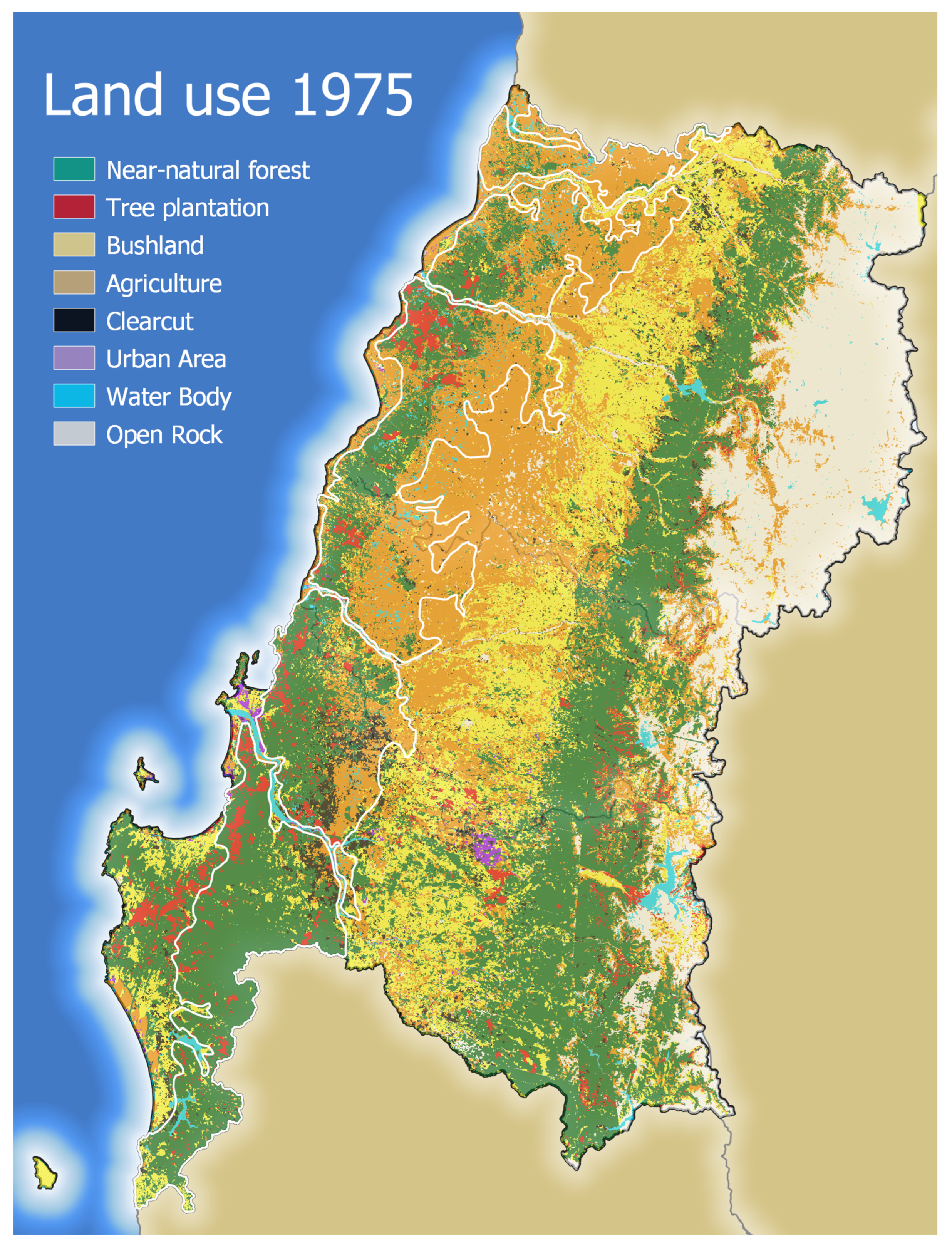
Figure A2.
Land use map of study site in 1980.
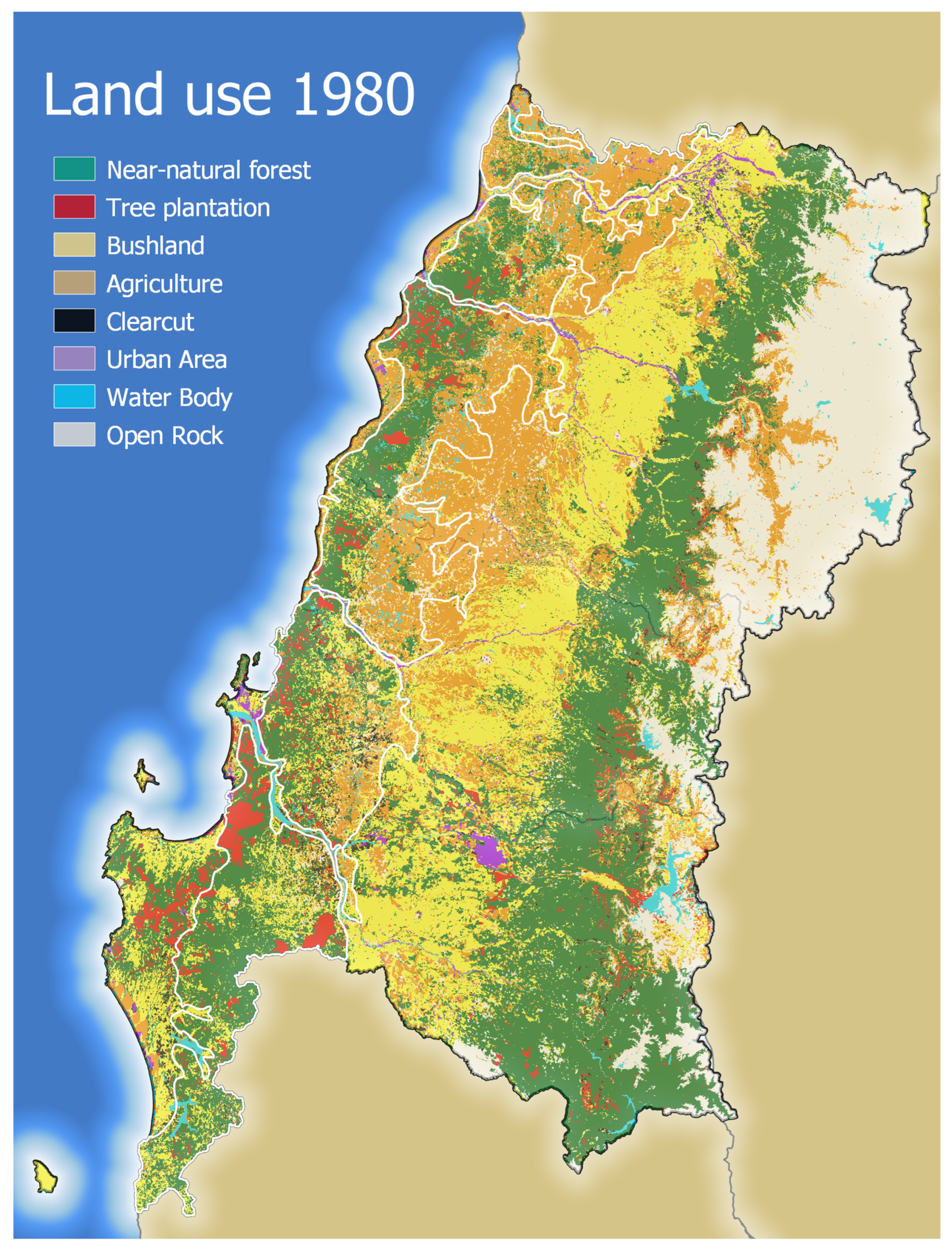
Figure A3.
Land use map of study site in 1985.
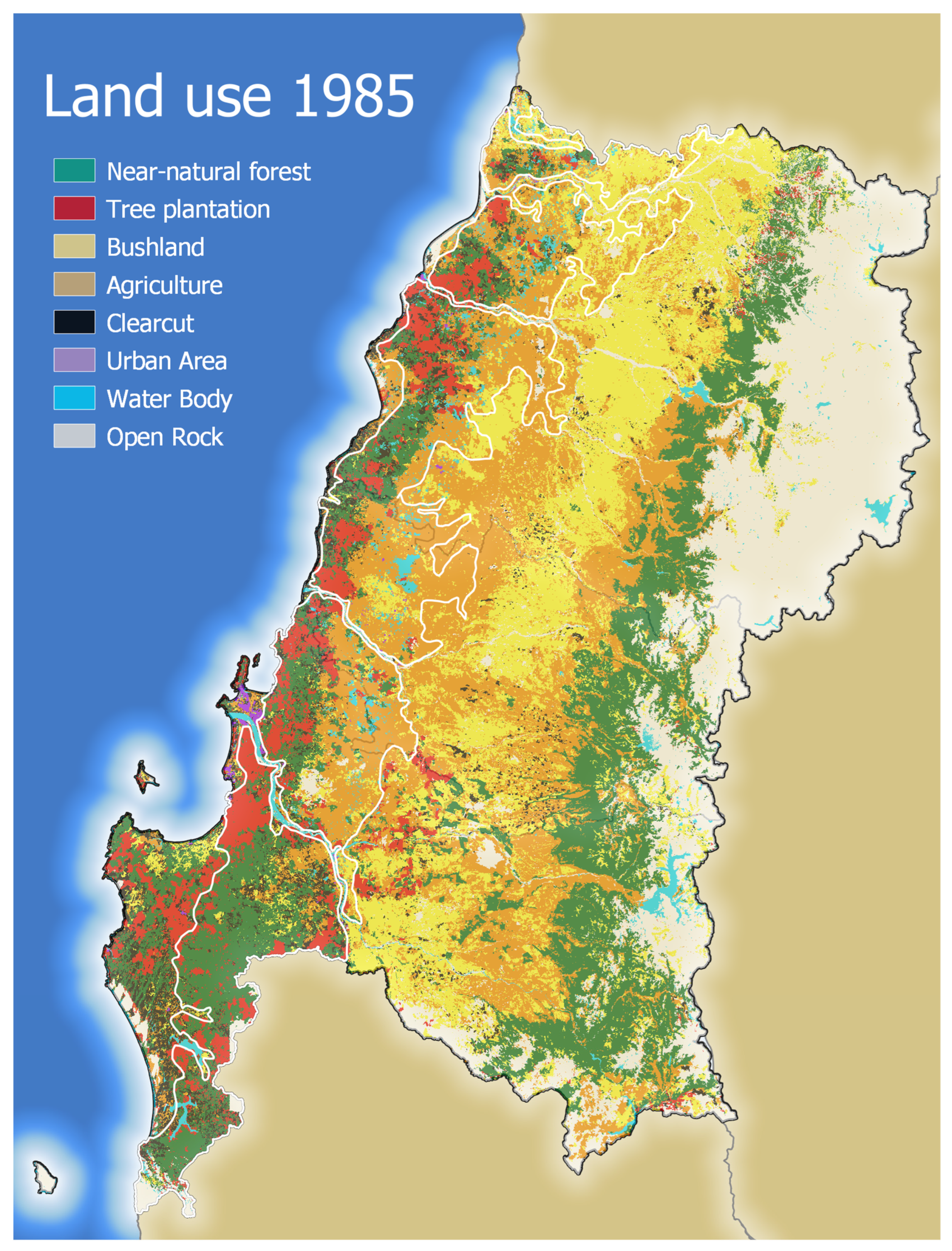
Figure A4.
Land use map of study site in 1990.

Figure A5.
Land use map of study site in 1995.
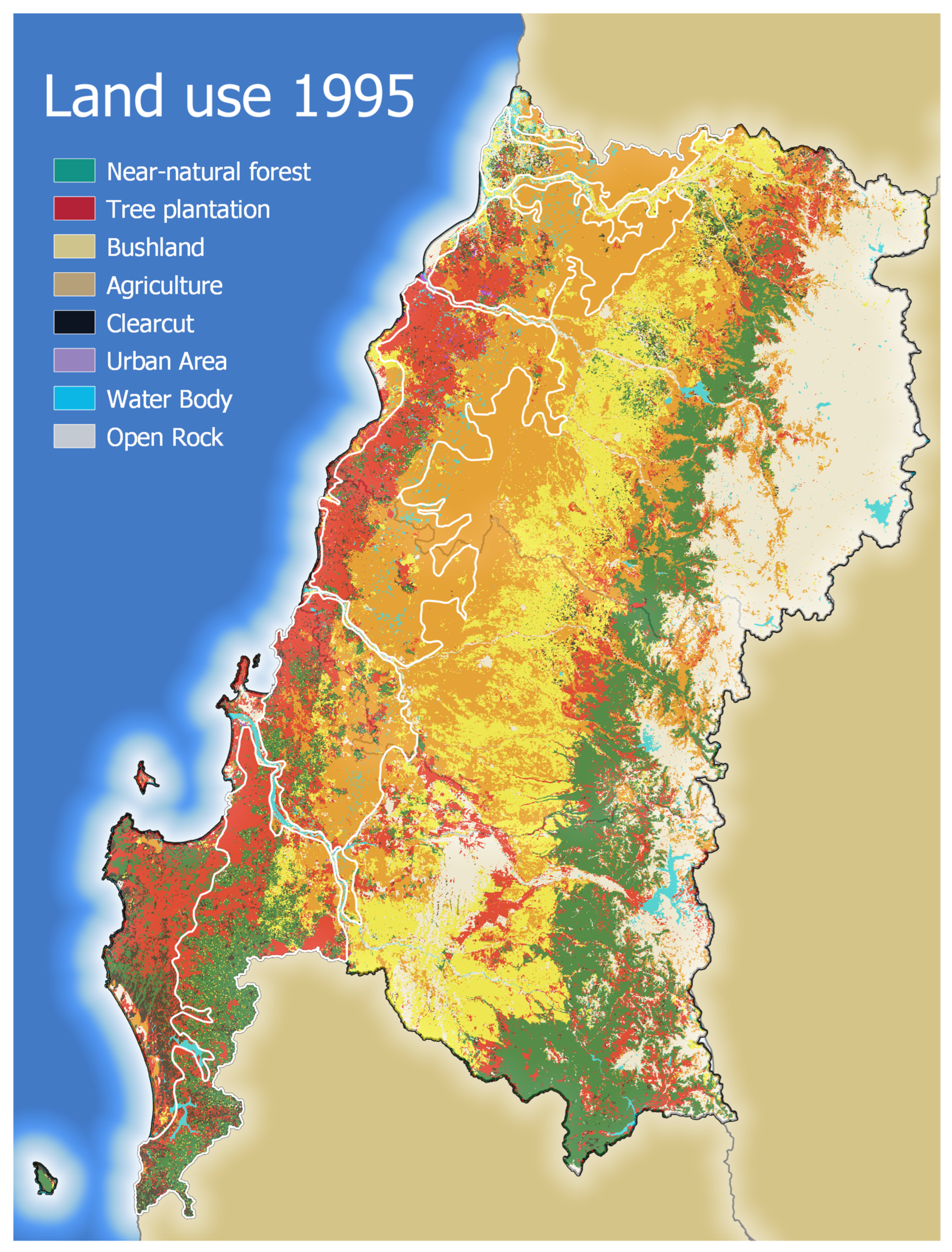
Figure A6.
Land use map of study site in 1995.

Figure A7.
Land use map of study site in 2005.
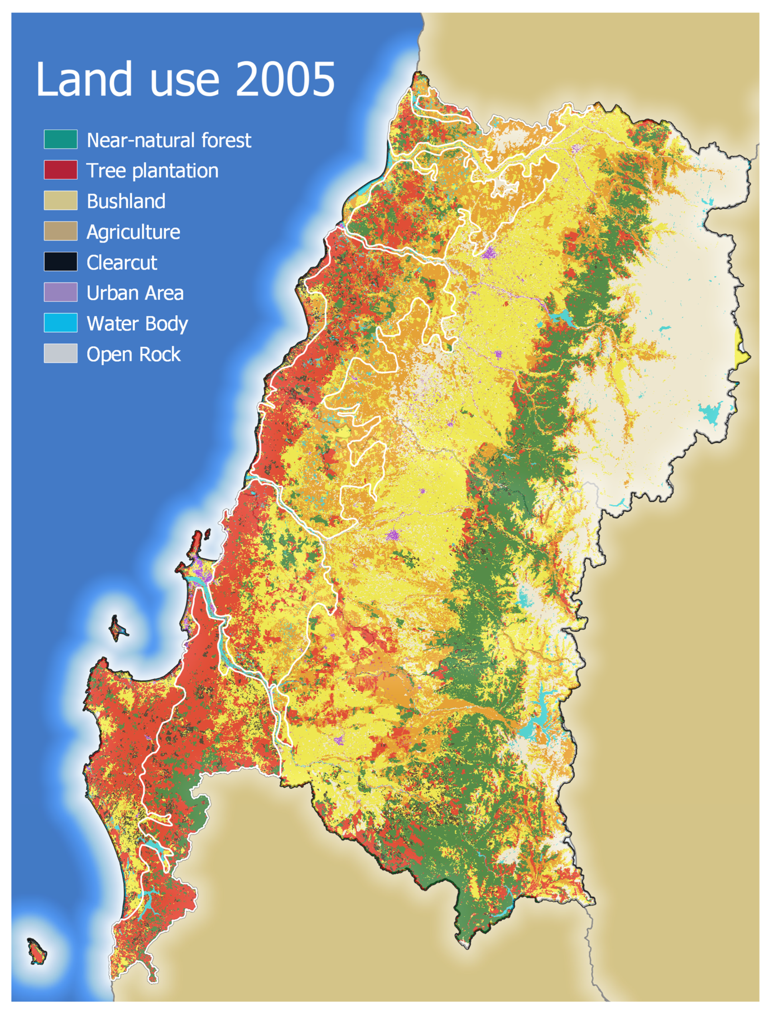
Figure A8.
Land use map of study site in 2010.
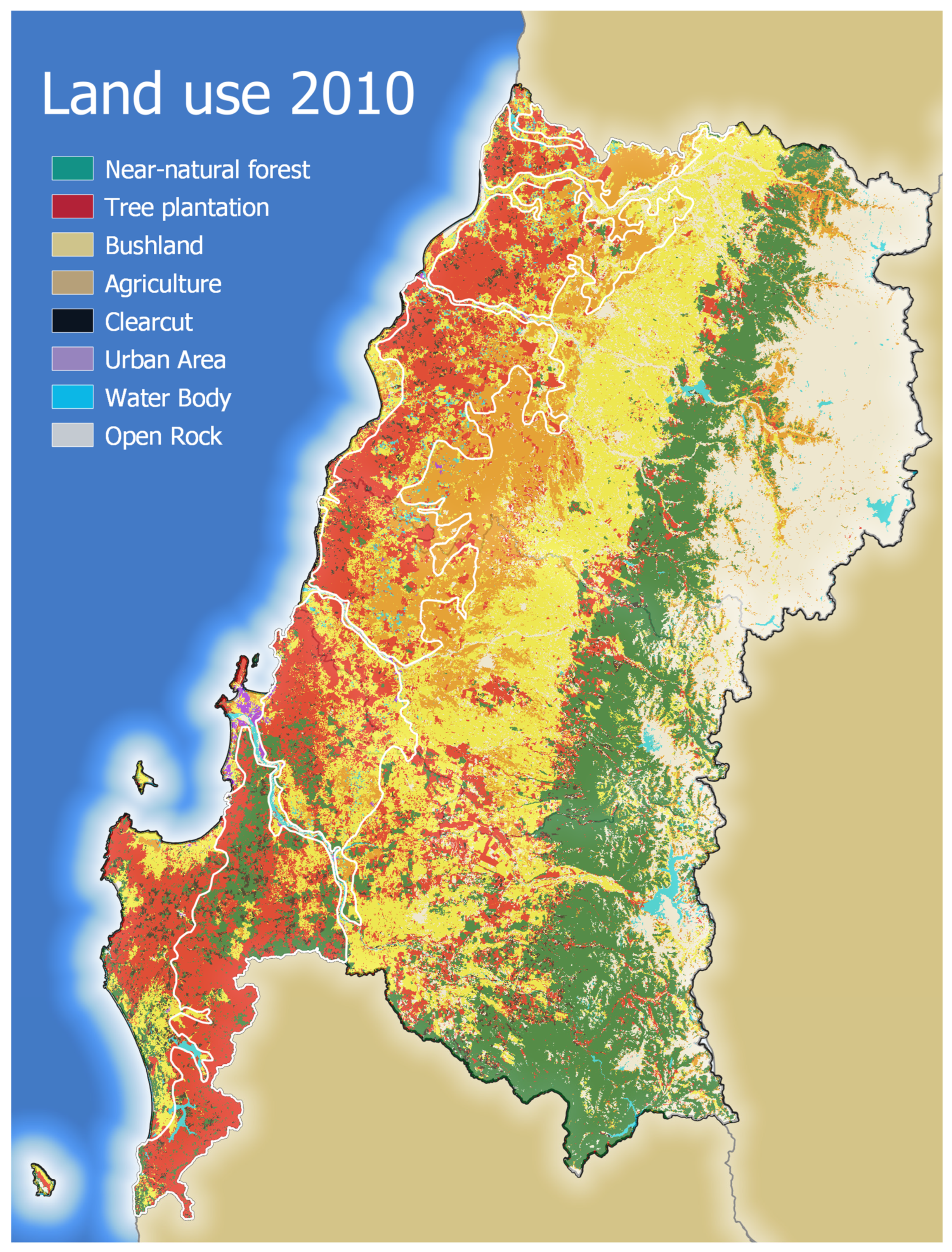
Appendix F
Figure A9.
Overview of the area in the northern study area (small white inset in Figure 3). This section shows the land use change particularly clearly. It shows the area where plantations were already present in 1975. These are some of the first plantations estab.
Figure A9.
Overview of the area in the northern study area (small white inset in Figure 3). This section shows the land use change particularly clearly. It shows the area where plantations were already present in 1975. These are some of the first plantations estab.
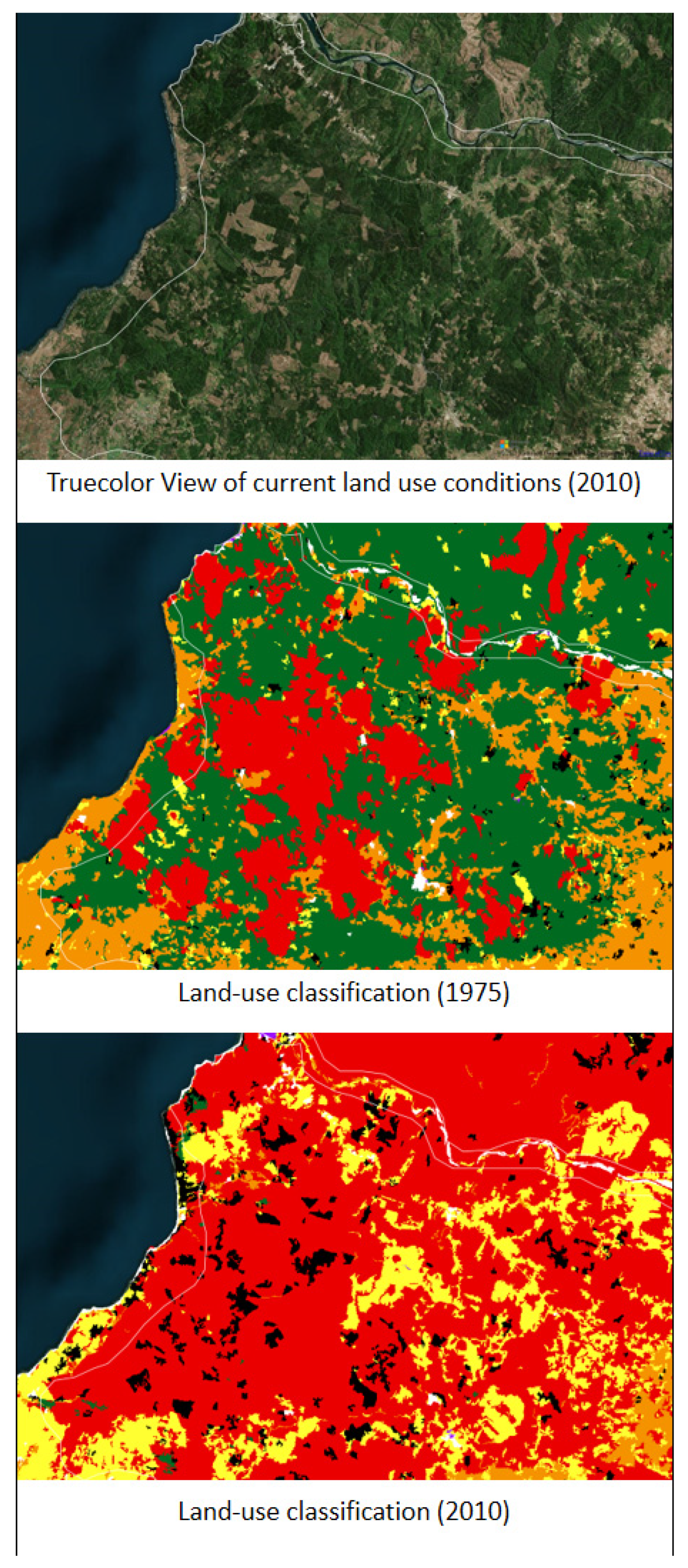
References
- Song, X.-P.; Hansen, M.C.; Stehman, S.V.; Potapov, P.V.; Tyukavina, A.; Vermote, E.F.; Townshend, J.R. Global land change from 1982 to 2016. Nature 2018, 560, 639–643. [Google Scholar] [CrossRef] [PubMed]
- Turner, B.L. Local faces, global flows: The role of land use and land cover in global environmental change. Land Degrad. Dev. 1994, 5, 71–78. [Google Scholar] [CrossRef]
- Dirmeyer, P.; Niyogi, D.; De Noblet-Ducoudré, N.; Dickinson, R.E.; Snyder, P.K. Impacts of land use change on climate. Int. J. Clim. 2010, 30, 1905–1907. [Google Scholar] [CrossRef] [Green Version]
- Pouyat, R.V.; Pataki, D.E.; Belt, K.T.; Groffman, P.M.; Hom, J.; Band, L.E. Effects of urban land-use change on biogeochemical cycles. In Terrestrial Ecosystems in a Changing World; Springer: Berlin/Heidelberg, Germany, 2007; pp. 45–58. [Google Scholar] [CrossRef]
- De Jong, L.; De Bruin, S.; Knoop, J.; van Vliet, J. Understanding land-use change conflict: A systematic review of case studies. J. Land Use Sci. 2021, 16, 223–239. [Google Scholar] [CrossRef]
- Sloan, S.; Sayer, J.A. Forest Resources Assessment of 2015 shows positive global trends but forest loss and degradation persist in poor tropical countries. For. Ecol. Manag. 2015, 352, 134–145. [Google Scholar] [CrossRef] [Green Version]
- Buongiorno, J.; Zhu, S. Assessing the impact of planted forests on the global forest economy. N. Zeal. J. For. Sci. 2014, 44, S2. [Google Scholar] [CrossRef] [Green Version]
- Doelman, J.C.; Stehfest, E.; van Vuuren, D.P.; Tabeau, A.; Hof, A.F.; Braakhekke, M.C.; Gernaat, D.E.H.J.; Berg, M.V.D.; van Zeist, W.; Daioglou, V.; et al. Afforestation for climate change mitigation: Potentials, risks and trade-offs. Glob. Chang. Biol. 2019, 26, 1576–1591. [Google Scholar] [CrossRef]
- Payn, T.; Carnus, J.-M.; Freer-Smith, P.; Kimberley, M.; Kollert, W.; Liu, S.; Orazio, C.; Rodriguez, L.; Silva, L.N.; Wingfield, M.J. Changes in planted forests and future global implications. For. Ecol. Manag. 2015, 352, 57–67. [Google Scholar] [CrossRef] [Green Version]
- Schirmer, J. Plantations and social conflict: Exploring the differences between small-scale and large-scale plantation forestry. Small Scale For. 2007, 6, 19–33. [Google Scholar] [CrossRef]
- Gerber, J.-F. Conflicts over industrial tree plantations in the South: Who, how and why? Glob. Environ. Chang. 2011, 21, 165–176. [Google Scholar] [CrossRef]
- Malkamäki, A.; D’Amato, D.; Hogarth, N.; Kanninen, M.; Pirard, R.; Toppinen, A.; Zhou, W. A systematic review of the socio-economic impacts of large-scale tree plantations, worldwide. Glob. Environ. Chang. 2018, 53, 90–103. [Google Scholar] [CrossRef]
- Valduga, M.O.; Zenni, R.D.; Vitule, J.R. Ecological impacts of non-native tree species plantations are broad and heterogeneous: A review of Brazilian research. An. Da Acad. Bras. De Ciências 2016, 88, 1675–1688. [Google Scholar] [CrossRef] [PubMed] [Green Version]
- Dodet, M.; Collet, C. When should exotic forest plantation tree species be considered as an invasive threat and how should we treat them? Biol. Invasions 2012, 14, 1765–1778. [Google Scholar] [CrossRef]
- Farley, K.A.; Jobbagy, E.G.; Jackson, R.B. Effects of afforestation on water yield: A global synthesis with implications for policy. Glob. Chang. Biol. 2005, 11, 1565–1576. [Google Scholar] [CrossRef]
- Honegger, M.; Michaelowa, A.; Roy, J. Potential implications of carbon dioxide removal for the sustainable development goals. Clim. Policy 2020, 21, 678–698. [Google Scholar] [CrossRef]
- Bull, G.Q.; Bazett, M.; Schwab, O.; Nilsson, S.; White, A.; Maginnis, S. Industrial forest plantation subsidies: Impacts and implications. For. Policy Econ. 2006, 9, 13–31. [Google Scholar] [CrossRef]
- Clapp, R.A. The Unnatural History of the Monterey Pine. Geogr. Rev. 1995, 85, 1–19. [Google Scholar] [CrossRef]
- Hofflinger, A.; Nahuelpan, H.; Boso, À.; Millalen, P. Do Large-Scale Forestry Companies Generate Prosperity in Indigenous Communities? The Socioeconomic Impacts of Tree Plantations in Southern Chile. Hum. Ecol. 2021, 49, 619–630. [Google Scholar] [CrossRef]
- Clapp, R.A. Creating Competitive Advantage: Forest Policy as Industrial Policy in Chile. Econ. Geogr. 1995, 71, 273. [Google Scholar] [CrossRef]
- Langenfeld, M. Waldpolitik in Costa Rica und Chile; Springer: Fachmedien, Wiesbaden, 2017. [Google Scholar] [CrossRef]
- Grez, A.; Bustamante, R.; Simonetti, J.; Fahrig, L. Landscape Ecology, Deforestation, and forEst Fragmentation: The Case of the Ruil Forest in Chile: Landscape Ecology as a Tool for Sustainable Development in Latin America. 1998. Available online: https://www.researchgate.net/profile/aa-grez/publication/254319278_landscape_ecology_deforestation_and_forest_fragmentation_the_case_of_the_ruil_forest_in_chile/links/54c91abb0cf2595d6c7dfae5/landscape-ecology-deforestation-and-forest-fragmentation-the-case-of-the-ruil-forest-in-chile.pdf (accessed on 12 May 2021).
- Lara, A.; Urrutia, R.; Little, C.; Martinez, A. Servicios ecosistémicos y ley del bosque nativo: No basta con definirlos. Rev. Bosque Nativ. 2010, 47, 3–9. [Google Scholar]
- Tricallotis, M. ¿En qué contexto surge la certificación forestal en Chile?: Desempeño ambiental, social y económico de empresas no certificadas. Bosque 2016, 37, 613–624. [Google Scholar] [CrossRef] [Green Version]
- Clapp, R.A. Tree Farming and Forest Conservation in Chile: Do Replacement Forests Leave Any Originals Behind? Soc. Nat. Resour. 2001, 14, 341–356. [Google Scholar] [CrossRef]
- Aguayo, M.; Pauchard, A.; Azocar, G.; Parra, O. Land use change in the south central Chile at the end of the 20th century: Understanding the spatio-temporal dynamics of the landscape. Rev. Chil. De Hist. Nat. 2003, 82, 361–374. [Google Scholar]
- Echeverria, C.; Coomes, D.; Salas, J.; Benayas, J.R.; Lara, A.; Newton, A. Rapid deforestation and fragmentation of Chilean Temperate Forests. Biol. Conserv. 2006, 130, 481–494. [Google Scholar] [CrossRef]
- Schulz, J.J.; Cayuela, L.; Echeverria, C.; Salas, J.; Rey Benayas, J.M. Monitoring land cover change of the dryland forest landscape of Central Chile (1975–2008). Appl. Geogr. 2010, 30, 436–447. [Google Scholar] [CrossRef] [Green Version]
- Vergara, P.M.; Pérez-Hernández, C.G.; Hahn, I.J.; Soto, G.E. Deforestation in central Chile causes a rapid decline in landscape connectivity for a forest specialist bird species. Ecol. Res. 2013, 28, 481–492. [Google Scholar] [CrossRef]
- Altamirano, A.; Lara, A. Deforestation in temperate ecosystems of pre-Andean range of south-central Chile. Bosque 2010, 31, 53–64. [Google Scholar]
- Altamirano, A.; Aplin, P.; Miranda, A.; Cayuela, L.; Algar, A.C.; Field, R. High rates of forest loss and turnover obscured by classical landscape measures. Appl. Geogr. 2013, 40, 199–211. [Google Scholar] [CrossRef]
- Miranda, A.; Altamirano, A.; Cayuela, L.; Pincheira, F.; Lara, A. Different times, same story: Native forest loss and landscape homogenization in three physiographical areas of south-central of Chile. Appl. Geogr. 2015, 60, 20–28. [Google Scholar] [CrossRef]
- Zamorano-Elgueta, C.; Benayas, J.R.; Cayuela, L.; Hantson, S.; Armenteras, D. Native forest replacement by exotic plantations in southern Chile (1985–2011) and partial compensation by natural regeneration. For. Ecol. Manag. 2015, 345, 10–20. [Google Scholar] [CrossRef] [Green Version]
- Echeverría, C.; Newton, A.; Nahuelhual, L.; Coomes, D.; Benayas, J.R. How landscapes change: Integration of spatial patterns and human processes in temperate landscapes of southern Chile. Appl. Geogr. 2012, 32, 822–831. [Google Scholar] [CrossRef]
- Heilmayr, R.; Echeverría, C.; Fuentes, R.; Lambin, E.F. A plantation-dominated forest transition in Chile. Appl. Geogr. 2016, 75, 71–82. [Google Scholar] [CrossRef] [Green Version]
- Mather, A.S. The forest transition. Area 1992, 367–379. Available online: https://www.jstor.org/stable/20003181 (accessed on 12 May 2021).
- Uribe, S.V.; Estades, C.; Radeloff, V.C. Pine plantations and five decades of land use change in central Chile. PLoS ONE 2020, 15, e0230193. [Google Scholar] [CrossRef] [Green Version]
- Nahuelhual, L.; Carmona, A.; Lara, A.; Echeverría, C.; González, M.E. Land-cover change to forest plantations: Proximate causes and implications for the landscape in south-central Chile. Landsc. Urban Plan. 2012, 107, 12–20. [Google Scholar] [CrossRef] [Green Version]
- Miranda, A.; Altamirano, A.; Cayuela, L.; Lara, A.; González, M. Native forest loss in the Chilean biodiversity hotspot: Revealing the evidence. Reg. Environ. Chang. 2016, 17, 285–297. [Google Scholar] [CrossRef]
- Lanfranco, D.; Dungey, H.S. Insect damage in Eucalyptus: A review of plantations in Chile. Austral Ecol. 2001, 26, 477–481. [Google Scholar] [CrossRef]
- Lara, A.; Jones, J.; Little, C.; Vergara, N. Streamflow response to native forest restoration in former Eucalyptus plantations in south central Chile. Hydrol. Process. 2021, 35, e14270. [Google Scholar] [CrossRef]
- Huber, A.; Iroumé, A.; Mohr, C.; Frêne, C. Efecto de plantaciones de Pinus radiata y Eucalyptus globulus sobre el recurso agua en la Cordillera de la Costa de la región del Biobío, Chile. Bosque 2010, 31, 219–230. [Google Scholar] [CrossRef]
- McWethy, D.B.; Pauchard, A.; García, R.A.; Holz, A.; González, M.E.; Veblen, T.T.; Stahl, J.; Currey, B. Landscape drivers of recent fire activity (2001–2017) in south-central Chile. PLoS ONE 2018, 13, e0201195. [Google Scholar] [CrossRef]
- Garreaud, R.D.; Boisier, J.P.; Rondanelli, R.; Montecinos, A.; Sepúlveda, H.H.; Veloso-Aguila, D. The Central Chile Mega Drought (2010–2018): A climate dynamics perspective. Int. J. Clim. 2019, 40, 421–439. [Google Scholar] [CrossRef]
- Braun, A.C.; Faßnacht, F.; Valencia, D.; Sepulveda, M. Consequences of land-use change and the wildfire disaster of 2017 for the central Chilean biodiversity hotspot. Reg. Environ. Chang. 2021, 21, 1–22. [Google Scholar] [CrossRef]
- Liu, X.; Andersson, C. Assessing the impact of temporal dynamics on land-use change modeling. Comput. Environ. Urban Syst. 2004, 28, 107–124. [Google Scholar] [CrossRef]
- Mas, J.-F.; De Vasconcelos, R.N.; Franca-Rocha, W. Analysis of High Temporal Resolution Land Use/Land Cover Trajectories. Land 2019, 8, 30. [Google Scholar] [CrossRef] [Green Version]
- Toro, J.; Gessel, S. Radiata pine plantations in Chile. New For. 1999, 18, 33–44. [Google Scholar] [CrossRef]
- Braun, A.C. More accurate less meaningful? A critical physical geographer’s reflection on interpreting remote sensing land-use analyses. Prog. Phys. Geogr. Earth Environ. 2021, 45, 706–735. [Google Scholar] [CrossRef]
- Braun, A.C.; Rojas, C.; Echeverria, C.; Rottensteiner, F.; Bahr, H.-P.; Niemeyer, J.; Arias, M.A.; Kosov, S.; Hinz, S.; Weidner, U. Design of a Spectral–Spatial Pattern Recognition Framework for Risk Assessments Using Landsat Data—A Case Study in Chile. IEEE J. Sel. Top. Appl. Earth Obs. Remote Sens. 2014, 7, 917–928. [Google Scholar] [CrossRef]
- Shao, G.; Wu, J. On the accuracy of landscape pattern analysis using remote sensing data. Landsc. Ecol. 2008, 23, 505–511. [Google Scholar] [CrossRef]
- Camus Gayan, P. De la panacea a la tragedia. Bosques, erosión y forestación en Chile. Siglos XIX y XX. HIB: Rev. De Hist. Iberoam. 2014, 7, 1. [Google Scholar] [CrossRef]
- Modrego, F.; Barrera, D.; Charnay, R. Estimacion del effecto del decreto ley N 701 de fomento forestal so-bre las tasas de forestación en Chile: Un análisis a nivel regional. Working Paper 2004. Available online: https://www.rimisp.org/wp-content/files_mf/135937542015.pdf (accessed on 12 May 2021).
- Altieri, M.A.; Rojas, A. Ecological Impacts of Chile’s Neoliberal Policies, with Special Emphasis on Agroecosystems. Environ. Dev. Sustain. 1999, 1, 55–72. [Google Scholar] [CrossRef]
- Asmüssen, M.V.; Simonetti, J.A. Can a developing country like Chile invest in biodiversity conservation? Environ. Conserv. 2007, 34, 183–185. [Google Scholar] [CrossRef]
- Banfield, C.C.; Braun, A.C.; Barra, R.; Castillo, A.; Vogt, J. Erosion proxies in an exotic tree plantation question the appropriate land use in Central Chile. CATENA 2018, 161, 77–84. [Google Scholar] [CrossRef]
- Aburto, F.; Cartes, E.; Mardones, O.; Rubilar, R. Hillslope soil erosion and mobility in pine plantations and native deciduous forest in the coastal range of south-Central Chile. Land Degrad. Dev. 2020, 32, 453–466. [Google Scholar] [CrossRef]
- Van Holt, T.; Moreno, C.A.; Binford, M.W.; Portier, K.M.; Mulsow, S.; Frazer, T.K. Influence of landscape change on nearshore fisheries in southern Chile. Glob. Chang. Biol. 2012, 18, 2147–2160. [Google Scholar] [CrossRef]
- Andersson, K.; Lawrence, D.; Zavaleta, J.; Guariguata, M.R. More Trees, More Poverty? The Socioeconomic Effects of Tree Plantations in Chile, 2001–2011. Environ. Manag. 2015, 57, 123–136. [Google Scholar] [CrossRef] [Green Version]
- Braun, A.C. Encroached by pine and eucalyptus? A grounded theory on an environmental conflict between forest industry and smallholder livelihoods in Chile. J. Rural Stud. 2021, 82, 107–120. [Google Scholar] [CrossRef]
- Lewis, S.L.; Wheeler, C.E.; Mitchard, E.T.A.; Koch, A. Restoring natural forests is the best way to remove atmospheric carbon. Nature 2019, 568, 25–28. [Google Scholar] [CrossRef]
- Braun, A.C.; Weidner, U.; Hinz, S. Classification in High-Dimensional Feature Spaces—Assessment Using SVM, IVM and RVM With Focus on Simulated EnMAP Data. IEEE J. Sel. Top. Appl. Earth Obs. Remote Sens. 2012, 5, 436–443. [Google Scholar] [CrossRef]
- Braun, A.C.; Weidner, U.; Hinz, S. Support Vector Machines for Vegetation Classification A Revision. Photogramm. Fernerkund. Geoinf. 2010, 2010, 273–281. [Google Scholar] [CrossRef]
- Urrutia-Jalabert, R.; Gonzalez, M.; González-Reyes, Á.; Lara, A.; Garreaud, R. Climate variability and forest fires in central and south-central Chile. Ecosphere 2018, 9, 1–17. [Google Scholar] [CrossRef]
- Acuña, E.; Sanfuentes, E.; Cancino, J.; Mena, P. Damage to remaining trees by four systems of mechanized harvest in commercial thinning of Pinus radiata. Ciência Florest. 2018, 28, 1317–1327. [Google Scholar] [CrossRef] [Green Version]
- UNECE/FAO. Chile’s Forest Products Markets-a Plantation Success Story. 2002. Available online: https://scholar.google.de/citations?user=znihdekaaaaj&hl=de&oi=sra (accessed on 12 May 2021).
- Salas-Eljatib, C.; Donoso, P.J.; Vargas, R.; Arriagada, C.A.; Pedraza, R.; Soto, D.P. The Forest Sector in Chile: An Overview and Current Challenges. J. For. 2016, 114, 562–571. [Google Scholar] [CrossRef] [Green Version]
- Cerda, R.; Gallardo-Cobos, R.; Sánchez-Zamora, P. An Analysis of the Impact of Forest Policy on Rural Areas of Chile. Forests 2020, 11, 1105. [Google Scholar] [CrossRef]
- Richter, R.; Schläpfer, D. Atmospheric and Topographic Correction (ATCOR Theoretical Background Document). DLR IB 2019, 564-03. Available online: http://www.rese-apps.com/pdf/atcor_atbd.pdf (accessed on 12 May 2021).
- Slater, J.A.; Heady, B.; Kroenung, G.; Curtis, W.; Haase, J.; Hoegemann, D.; Shockley, C.; Tracy, K. Global Assessment of the New ASTER Global Digital Elevation Model: American Society for Pho-togrammetry and Remote Sensing. Photogramm. Eng. Remote Sens. 2011, 77, 335–349. Available online: https://www.ingentaconnect.com/content/asprs/pers/2011/00000077/00000004/art00002 (accessed on 12 May 2021). [CrossRef]
- Weidner, U. Toward a framework for quality assessment in remote sensing applications. In Object and Pat-tern Recognition in Remote Sensing-Modelling and Monitoring Enviromental and Anthropogenic Objects and Change Processes; Hinz, S., Braun, A., Weinmann, M., Eds.; Whittles Publishing: Dunbeath, Scotland, 2021. [Google Scholar]
- Kraemer, H.C. Kappa Coefficient. In Wiley StatsRef: Statistics Reference Online; John Wiley & Sons, Ltd.: Hoboken, NJ, USA, 2015; pp. 1–4. [Google Scholar]
- Kattenborn, T.; Lopatin, J.; Förster, M.; Braun, A.C.; Fassnacht, F.E. UAV data as alternative to field sampling to map woody invasive species based on combined Sentinel-1 and Sentinel-2 data. Remote Sens. Environ. 2019, 227, 61–73. [Google Scholar] [CrossRef]
- Xie, Y.; Sha, Z.; Yu, M. Remote sensing imagery in vegetation mapping: A review. J. Plant Ecol. 2008, 1, 9–23. [Google Scholar] [CrossRef]
- Shoshany, M. Satellite remote sensing of natural Mediterranean vegetation: A review within an ecological context. Prog. Phys. Geogr. Earth Environ. 2000, 24, 153–178. [Google Scholar] [CrossRef]
- Kattenborn, T.; Leitloff, J.; Schiefer, F.; Hinz, S. Review on Convolutional Neural Networks (CNN) in vegetation remote sensing. ISPRS J. Photogramm. Remote Sens. 2021, 173, 24–49. [Google Scholar] [CrossRef]
- Fu, Y.; Zhao, C.; Wang, J.; Jia, X.; Yang, G.; Song, X.; Feng, H. An Improved Combination of Spectral and Spatial Features for Vegetation Classification in Hyperspectral Images. Remote Sens. 2017, 9, 261. [Google Scholar] [CrossRef] [Green Version]
- Ashoori, H.; Zoej, M.J.V.; Sahebi, M.R. Introduction of Spatio-Spectral Indices for Using Spatial Data in Multispectral Image Classification. J. Indian Soc. Remote Sens. 2019, 47, 1003–1017. [Google Scholar] [CrossRef]
- Object and Pattern Recognition in Remote Sensing-Modelling and Monitoring Enviromental and Anthropogenic Objects and Change Processes; Stefan, H.; Andreas, B.; Martin, W. (Eds.) Whittles Publishing: Dunbeath, Scotland, 2021; Available online: https://www.whittlespublishing.com/Object_and_Pattern_Recognition_in_Remote_Sensing_ (accessed on 12 May 2021).
- Fauvel, M.; Tarabalka, Y.; Benediktsson, J.A.; Chanussot, J.; Tilton, J.C. Advances in spectral-spatial classification of hyperspectral images. Proc. IEEE 2013, 101, 652–675. [Google Scholar] [CrossRef] [Green Version]
- Jimenez, L.; Landgrebe, D. Supervised classification in high-dimensional space: Geometrical, statistical, and asymptotical properties of multivariate data. IEEE Trans. Syst. Man Cybern. Part C Appl. Rev. 1998, 28, 39–54. [Google Scholar] [CrossRef]
- Altman, N.; Krzywinski, M. The curse(s) of dimensionality. Nat. Methods 2018, 15, 399–400. [Google Scholar] [CrossRef]
- Dalla Mura, M.; Benediktsson, J.A.; Waske, B.; Bruzzone, L. Morphological Attribute Profiles for the Analysis of Very High Resolution Images. IEEE Trans. Geosci. Remote Sens. 2010, 48, 3747–3762. [Google Scholar] [CrossRef]
- Whitley, D.C.; Ford, M.G.; Livingstone, D.J. Unsupervised Forward Selection: A Method for Eliminating Redundant Variables. J. Chem. Inf. Comput. Sci. 2000, 40, 1160–1168. [Google Scholar] [CrossRef] [PubMed]
- Yu, S.; Tranchevent, L.-C.; De Moor, B.; Moreau, Y. Kernel-Based Data Fusion for Machine Learning; Springer: Berlin, Germany, 2011. [Google Scholar]
- Braun, A.C.; Weidner, U.; Jutzi, B.; Hinz, S. Verknüpfung von Kernfunktionen mit der eins-gegen-eins Kaskade für die Einbindung von Wissen in die SVM Klassifizierung. Photogramm Fernerkund. Geoinf. 2012, 2012, 371–384. [Google Scholar] [CrossRef]
- Lee, W.-J.; Verzakov, S.; Duin, R.P. Kernel combination versus classifier combination. In International Workshop on Multiple Classifier Systems; Springer: Berlin/Heidelberg, Germany, 2007; Volume 4472, pp. 22–31. [Google Scholar]
- Szafranski, M.; Grandvalet, Y.; Rakotomamonjy, A. Composite kernel learning. Mach. Learn. 2009, 79, 73–103. [Google Scholar] [CrossRef] [Green Version]
- Braun, A.C.; Weidner, U.; Jutzi, B.; Hinz, S. Integrating external knowledge into SVM classification—Fusing hyperspectral and laserscanning data by kernel composition. ISPRS Int. Arch. Photogramm. Remote Sens. Spat. Inf. Sci. 2012, XXXVIII-4, 57–62. [Google Scholar] [CrossRef] [Green Version]
- Braun, A.C.; Weidner, U.; Hinz, S. Classifying roof materials using data fusion through kernel composi-tion—Comparing ν-SVM and one-class SVM. In Proceedings of the 2011 Joint Urban Remote Sensing Event, Munich, Germany, 11–13 April 2011; pp. 377–380. [Google Scholar]
- Camps-Valls, G.; Bruzzone, L. Kernel Methods for Remote Sensing Data Analysis; Wiley: West Sussex, UK, 2009. [Google Scholar]
- Wolpert, D.H.; Macready, W.G. No free lunch theorems for optimization. IEEE Trans. Evol. Comput. 1997, 1, 67–82. [Google Scholar] [CrossRef] [Green Version]
- Briem, G.; Benediktsson, J.A.; Sveinsson, J.R. Multiple classifiers applied to multisource remote sensing data. IEEE Trans. Geosci. Remote Sens. 2002, 40, 2291–2299. [Google Scholar] [CrossRef] [Green Version]
- Boser, B.E.; Guyon, I.M.; Vapnik, V.N. A training algorithm for optimal margin classifiers. In Proceedings of the Fifth Annual Workshop on Computational Learning Theory-COLT ‘92, New York, NY, USA, 27–29 July 1992. [Google Scholar]
- Zhu, J.; Hastie, T. Kernel Logistic Regression and the Import Vector Machine. J. Comput. Graph. Stat. 2005, 14, 185–205. [Google Scholar] [CrossRef]
- Tipping, M.E. Sparse Bayesian learning and the relevance vector machine. J. Mach. Learn. Re Search 2001, 1, 211–244. Available online: https://www.jmlr.org/papers/volume1/tipping01a/tipping01a.pdf (accessed on 12 May 2021).
- Chang, C.; Lin, C. LIBSVM: A Library for Support Vector Machines. ACM Trans. Intell. Syst. Technol. 2013, 2, 1–39. [Google Scholar] [CrossRef]
- Roscher, R.; Förstner, W.; Waske, B. I2VM: Incremental import vector machines. Image Vis. Comput. 2012, 30, 263–278. [Google Scholar] [CrossRef]
- Puyravaud, J.-P. Standardizing the calculation of the annual rate of deforestation. For. Ecol. Manag. 2003, 177, 593–596. [Google Scholar] [CrossRef]
- Salah, M.; Trinder, J.C.; Shaker, A.; Hamed, B.; Elsagheer, B. Integrating Multiple Classifiers with Fuzzy Majority Voting for Improved Land cover Classification. Available online: http://citeseerx.ist.psu.edu/viewdoc/summary?doi=10.1.1.367.2418 (accessed on 12 May 2021).
- Cohen, W.B.; Goward, S.N. Landsat’s Role in Ecological Applications of Remote Sensing. BioScience 2004, 54, 535. [Google Scholar] [CrossRef]
- Niemeyer, J.; Rottensteiner, F.; Soergel, U. Classification of urban LiDAR data using conditional random field and random forests. In Proceedings of the Joint Urban Remote Sensing Event, Sao Paolo, Brazil, 21–23 April 2013; pp. 139–142. [Google Scholar]
- Wang, M.; Zhang, H.; Sun, W.; Li, S.; Wang, F.; Yang, G. A Coarse-to-Fine Deep Learning Based Land Use Change Detection Method for High-Resolution Remote Sensing Images. Remote Sens. 2020, 12, 1933. [Google Scholar] [CrossRef]
- Mu, L.; Wang, L.; Wang, Y.; Chen, X.; Han, W. Urban Land Use and Land Cover Change Prediction via Self-Adaptive Cellular Based Deep Learning With Multisourced Data. IEEE J. Sel. Top. Appl. Earth Obs. Remote Sens. 2019, 12, 5233–5247. [Google Scholar] [CrossRef]
- Jozdani, S.E.; Johnson, B.A.; Chen, D. Comparing Deep Neural Networks, Ensemble Classifiers, and Support Vector Machine Algorithms for Object-Based Urban Land Use/Land Cover Classification. Remote Sens. 2019, 11, 1713. [Google Scholar] [CrossRef] [Green Version]
- Liu, P.; Choo, K.-K.R.; Wang, L.; Huang, F. SVM or deep learning? A comparative study on remote sensing image classification. Soft Comput. 2016, 21, 7053–7065. [Google Scholar] [CrossRef]
- Hasan, H.; Shafri, H.Z.; Habshi, M. A Comparison Between Support Vector Machine (SVM) and Convolutional Neural Network (CNN) Models For Hyperspectral Image Classification. IOP Conf. Series Earth Environ. Sci. 2019, 357, 012035. [Google Scholar] [CrossRef] [Green Version]
- Heilmayr, R.; Echeverría, C.; Lambin, E.F. Impacts of Chilean forest subsidies on forest cover, carbon and biodiversity. Nat. Sustain 2020, 3, 701–709. [Google Scholar] [CrossRef]
- Pannell, D.J.; Roberts, A.M. Conducting and delivering integrated research to influence land-use policy: Salinity policy in Australia. Environ. Sci. Policy 2009, 12, 1088–1098. [Google Scholar] [CrossRef]
- Sohl, T.L.; Claggett, P.R. Clarity versus complexity: Land-use modeling as a practical tool for decision-makers. J. Environ. Manag. 2013, 129, 235–243. [Google Scholar] [CrossRef]
- De Oca, A.I.F.-M.; Gallardo-Cruz, J.A.; Ghilardi, A.; Kauffer, E.; Solórzano, J.V.; Sánchez-Cordero, V. An integrated framework for harmonizing definitions of deforestation. Environ. Sci. Policy 2020, 115, 71–78. [Google Scholar] [CrossRef]
- Van Holt, T.; Binford, M.W.; Portier, K.M.; Vergara, R. A stand of trees does not a forest make: Tree plantations and forest transitions. Land Use Policy 2016, 56, 147–157. [Google Scholar] [CrossRef]
- Gachet, S.; Leduc, A.; Bergeron, Y.; Nguyen-Xuan, T.; Tremblay, F. Understory vegetation of boreal tree plantations: Differences in relation to previous land use and natural forests. For. Ecol. Manag. 2007, 242, 49–57. [Google Scholar] [CrossRef]
- Komatsu, H.; Kume, T.; Otsuki, K. The effect of converting a native broad-leaved forest to a coniferous plantation forest on annual water yield: A paired-catchment study in northern Japan. For. Ecol. Manag. 2008, 255, 880–886. [Google Scholar] [CrossRef]
- Braun, A.C.; Troeger, D.; Garcia, R.; Aguayo, M.; Barra, R.; Vogt, J. Assessing the impact of plantation forestry on plant biodiversity. Glob. Ecol. Conserv. 2017, 10, 159–172. [Google Scholar] [CrossRef]
- Baruch, Z.; Nozawa, S.; Johnson, E.; Yerena, E. Ecosystem dynamics and services of a paired Neotropical montane forest and pine plantation. Rev. Biol. Trop. 2019, 67, 24–35. [Google Scholar] [CrossRef]
- Perz, S.G. Grand Theory and Context-Specificity in the Study of Forest Dynamics: Forest Transition Theory and Other Directions. Prof. Geogr. 2007, 59, 105–114. [Google Scholar] [CrossRef]
- Langdon, B.; Pauchard, A.; Aguayo, M. Pinus contorta invasion in the Chilean Patagonia: Local patterns in a global context. Biol. Invasions 2010, 12, 3961–3971. [Google Scholar] [CrossRef]
- Paritsis, J.; Landesmann, J.B.; Kitzberger, T.; Tiribelli, F.; Sasal, Y.; Quintero, C.; DiMarco, R.D.; Barrios-García, M.N.; Iglesias, A.L.; Diez, J.P.; et al. Pine Plantations and Invasion Alter Fuel Structure and Potential Fire Behavior in a Patagonian Forest-Steppe Ecotone. Forests 2018, 9, 117. [Google Scholar] [CrossRef] [Green Version]
- Myers, N.; Mittermeier, R.A.; Mittermeier, C.G.; da Fonseca, G.A.B.; Kent, J. Biodiversity hotspots for conservation priorities. Nature 2000, 403, 853–858. [Google Scholar] [CrossRef] [PubMed]
- Rockström, J.; Steffen, W.; Noone, K.; Persson, Å.; Chapin, F.S., III; Lambin, E.F.; Lenton, T.M.; Scheffer, M.; Folke, C.; Schellnhuber, H.J.; et al. A safe operating space for humanity. Nature 2009, 461, 472–475. [Google Scholar] [CrossRef]
- Smith-Ramírez, C.; González, M.E.; Echeverría, C.; Lara, A. Estado actual de la restauración ecológica en Chile, perspectivas y desafíos: Current state of ecological restoration in Chile: Perspectives and challenges. An. Inst. Patagon. 2015, 43, 11–21. [Google Scholar] [CrossRef] [Green Version]
- Austin, K.G.; Schwantes, A.M.; Gu, Y.; Kasibhatla, P.S. What causes deforestation in Indonesia? Environ. Res. Lett. 2018, 14, 024007. [Google Scholar] [CrossRef]
- Danielsen, F.; Beukema, H.; Burgess, N.D.; Parish, F.; Brühl, C.A.; Donald, P.F.; Murdiyarso, D.; Phalan, B.; Reijnders, L.; Struebig, M.; et al. Biofuel Plantations on Forested Lands: Double Jeopardy for Biodiversity and Climate. Conserv. Biol. 2009, 23, 348–358. [Google Scholar] [CrossRef]
- Gaveau, D.L.A.; Sheil, D.; Husnayaen; Salim, M.A.; Arjasakusuma, S.; Ancrenaz, M.; Pacheco, P.; Meijaard, E. Rapid conversions and avoided deforestation: Examining four decades of industrial plantation expansion in Borneo. Sci. Rep. 2016, 6, 32017. [Google Scholar] [CrossRef] [PubMed]
- Vijay, V.; Pimm, S.L.; Jenkins, C.N.; Smith, S.J. The Impacts of Oil Palm on Recent Deforestation and Biodiversity Loss. PLoS ONE 2016, 11, e0159668. [Google Scholar] [CrossRef] [PubMed]
- Davis, K.; Yu, K.; Rulli, M.C.; Pichdara, L.; D’Odorico, P. Accelerated deforestation driven by large-scale land acquisitions in Cambodia. Nat. Geosci. 2015, 8, 772–775. [Google Scholar] [CrossRef] [Green Version]
- Scheidel, A.; Work, C. Large-Scale Forest Plantations for Climate Change Mitigation? New Frontiers of Deforestation and Land Grabbing in Cambodia. Glob. Gov. Politics Clim. Justice Agrar. Soc. Justice: Link. Chall. 2016, 11. Available online: https://www.tni.org/files/publication-downloads/11-icas_cp_scheidel_and_work.pdf (accessed on 12 May 2021).
- Jha, C.S.; Dutt, C.B.S.; Bawa, K.S. Deforestation and land use changes in Western Ghats, India. Curr. Sci. 2000, 231–238. [Google Scholar]
- Lohmann, L. Peasants, plantations, and pulp: The politics of eucalyptus in Thailand. Bull. Concerned Asian Sch. 1991, 23, 3–17. [Google Scholar] [CrossRef]
- Chidumayo, E.N. Land use, deforestation and reforestation in the Zambian Copperbelt. Land Degrad. Dev. 1989, 1, 209–216. [Google Scholar] [CrossRef]
- Chiti, T.; Grieco, E.; Perugini, L.; Rey, A.; Valentini, R. Effect of the replacement of tropical forests with tree plantations on soil organic carbon levels in the Jomoro district, Ghana. Plant Soil 2013, 375, 47–59. [Google Scholar] [CrossRef]
- Hajdu, F.; Penje, O.; Fischer, K. Questioning the use of ‘degradation’ in climate mitigation: A case study of a forest carbon CDM project in Uganda. Land Use Policy 2016, 59, 412–422. [Google Scholar] [CrossRef] [Green Version]
- Teucher, M.; Schmitt, C.B.; Wiese, A.; Apfelbeck, B.; Maghenda, M.; Pellikka, P.; Lens, L.; Habel, J.C. Behind the fog: Forest degradation despite logging bans in an east African cloud forest. Glob. Ecol. Conserv. 2020, 22, e01024. [Google Scholar] [CrossRef]
- Zurita, G.; Rey, N.; Varela, D.; Villagra, M.; Bellocq, M. Conversion of the Atlantic Forest into native and exotic tree plantations: Effects on bird communities from the local and regional perspectives. For. Ecol. Manag. 2006, 235, 164–173. [Google Scholar] [CrossRef]
- Heilmayr, R.; Lambin, E.F. Impacts of nonstate, market-driven governance on Chilean forests. Proc. Natl. Acad. Sci. USA 2016, 113, 2910–2915. [Google Scholar] [CrossRef] [PubMed] [Green Version]
- Edstedt, K.; Carton, W. The benefits that (only) capital can see? Resource access and degradation in industrial carbon forestry, lessons from the CDM in Uganda. Geoforum 2018, 97, 315–323. [Google Scholar] [CrossRef]
- Feilhauer, H.; Zlinszky, A.; Kania, A.; Foody, G.M.; Doktor, D.; Lausch, A.; Schmidtlein, S. Let your maps be fuzzy!—Class probabilities and floristic gradients as alternatives to crisp mapping for remote sensing of vegetation. Remote Sens. Ecol. Conserv. 2020, 7, 292–305. [Google Scholar] [CrossRef]
- Ji, C.; Heiden, U.; Lakes, T.; Feilhauer, H. Are urban material gradients transferable between areas? Int. J. Appl. Earth Obs. Geoinf. 2021, 100, 102332. [Google Scholar] [CrossRef]
- Ferchichi, A.; Boulila, W.; Farah, I.R. Propagating aleatory and epistemic uncertainty in land cover change prediction process. Ecol. Inform. 2017, 37, 24–37. [Google Scholar] [CrossRef] [Green Version]
- Moran, E.F. Environmental Social Science: Human-Environment Interactions and Sustainability; John Wiley & Sons: Malden, MA, USA, 2010. [Google Scholar]
- Reyes, R.; Nelson, H. A Tale of Two Forests: Why Forests and Forest Conflicts are Both Growing in Chile: Common-Wealth Forestry Association. 2014. Available online: https://www.ingentaconnect.com/content/cfa/ifr/2014/00000016/00000004/art00001 (accessed on 12 May 2021).
- Manuschevich, D.; Beier, C.M. Simulating land use changes under alternative policy scenarios for conservation of native forests in south-central Chile. Land Use Policy 2016, 51, 350–362. [Google Scholar] [CrossRef]
- Manuschevich, D.; Sarricolea, P.; Galleguillos, M. Integrating socio-ecological dynamics into land use policy outcomes: A spatial scenario approach for native forest conservation in south-central Chile. Land Use Policy 2019, 84, 31–42. [Google Scholar] [CrossRef]
- Arnold, F.E. Native Forest Policy in Chile: Understanding Sectoral Process Dynamics in a Country with an Emerging Economy: Commonwealth Forestry Association. 2003. Available online: https://www.ingentaconnect.com/content/cfa/ifr/2003/00000005/00000004/art00001 (accessed on 12 May 2021).
- Silva, E. The Political Economy of Forest Policy in Mexico and Chile. Singap. J. Trop. Geogr. 2004, 25, 261–280. [Google Scholar] [CrossRef]
- Cubbage, F.; Diaz, D.; Yapura, P.; Dube, F. Impacts of forest management certification in Argentina and Chile. For. Policy Econ. 2010, 12, 497–504. [Google Scholar] [CrossRef]
- Tricallotis, M.; Gunningham, N.; Kanowski, P. The impacts of forest certification for Chilean forestry businesses. For. Policy Econ. 2018, 92, 82–91. [Google Scholar] [CrossRef]
Figure 1.
Overview of the classification framework developed in Braun et al. [50] and employed herein in comparison to a standard workflow (Maximum Likelihood Classification). EMP: Extended Morphological Profile, Kernel Comp.: Kernel composition: SVM/IVM/RVM: Support/Import/Relevance Vector Machine, FMV-MCS: Fuzzy Majority Voting Multiple Classifier System, CRF: Conditional Random Field. Values in White Polygons: Accuracy Value A and increase of accuracy over comparison approach (Maximum Likelihood).
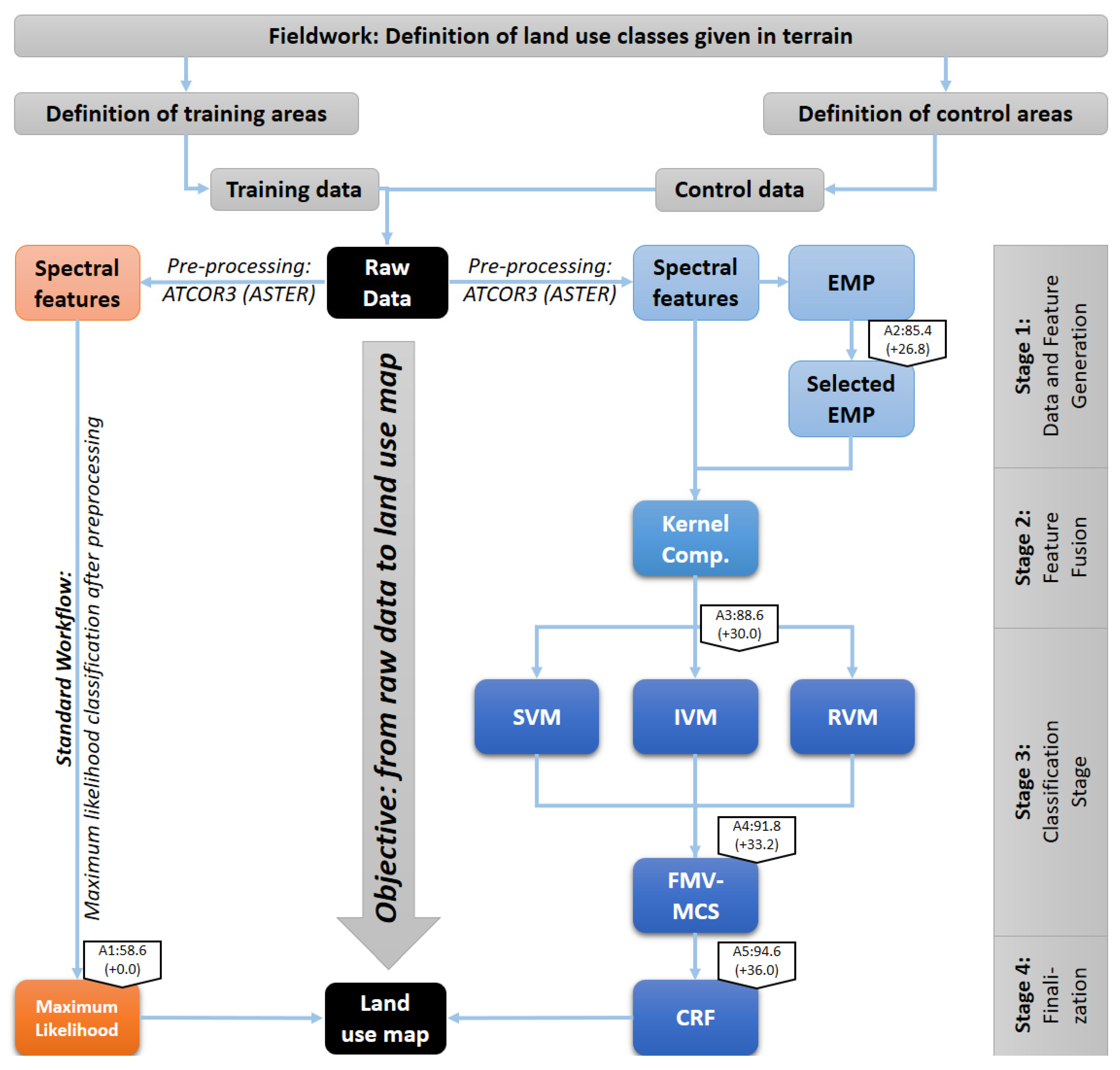
Figure 2.
Correspondence and non-correspondence of prospective and retrospective analysis. Upper part: Loss of LUS1 entirely in favor of LUS2, while LUS2 is established entirely at the cost of LUS1 (prospective analysis matches retrospective analysis). Lower part: Loss of LUS1 entirely in favor of LUS2, while LUS2 is predominantly established at the cost of LUS3 (the prospective analysis does not match retrospective analysis).
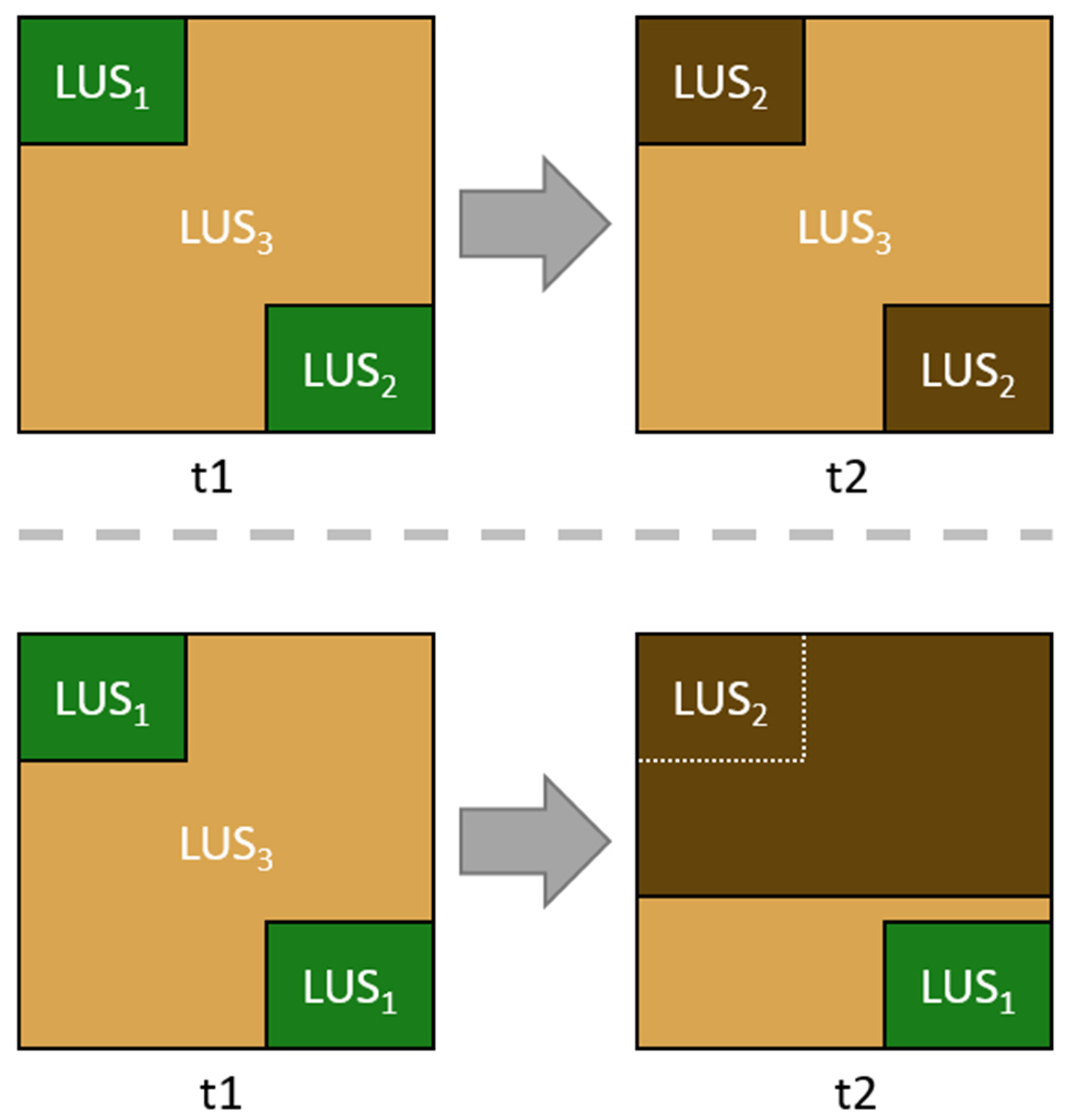
Figure 3.
Topographical overview of study site and land use maps for 1975 and 2015.
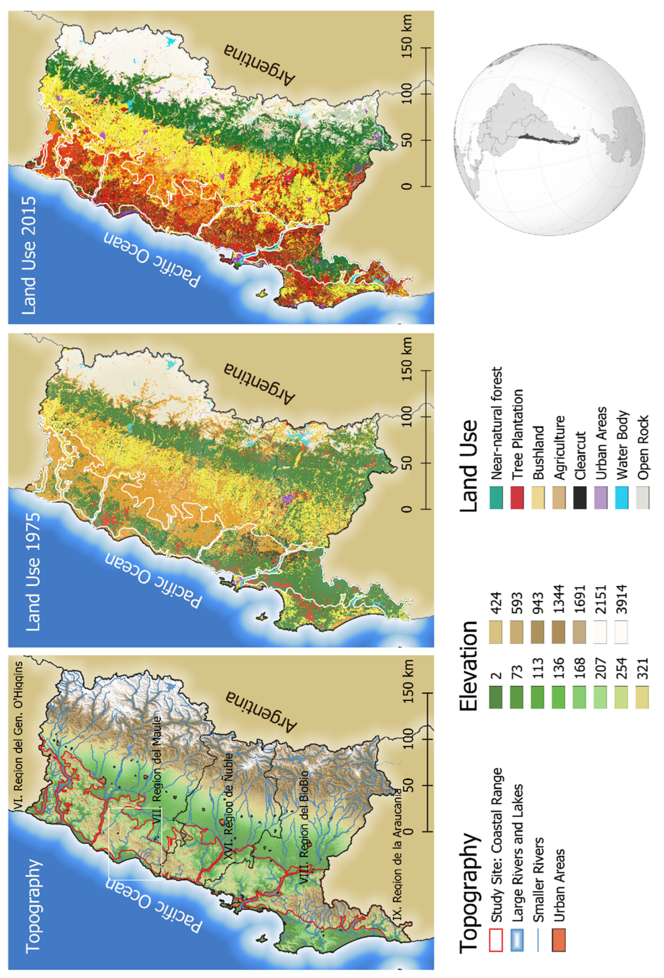
Figure 4.
(A) Percentages of main land use types (forest, plantation, bushlands, agriculture, clearcut) in five-year intervals, (B) Rates of deforestation of native forest and afforestation with industrial plantations in five-year intervals.
Figure 4.
(A) Percentages of main land use types (forest, plantation, bushlands, agriculture, clearcut) in five-year intervals, (B) Rates of deforestation of native forest and afforestation with industrial plantations in five-year intervals.

Figure 5.
Land use transitions. (A) Prospective analysis. Size of squares is proportional to the amount of land use of a particular type in 1975; width of lines is proportional to the amount of land use converted into another land use system in 2010. (B) Retrospective analysis. Size of squares is proportional to the amount of land use of a particular type in 2010; width of lines is proportional to the amount of land use taken from another land use system in 1975.
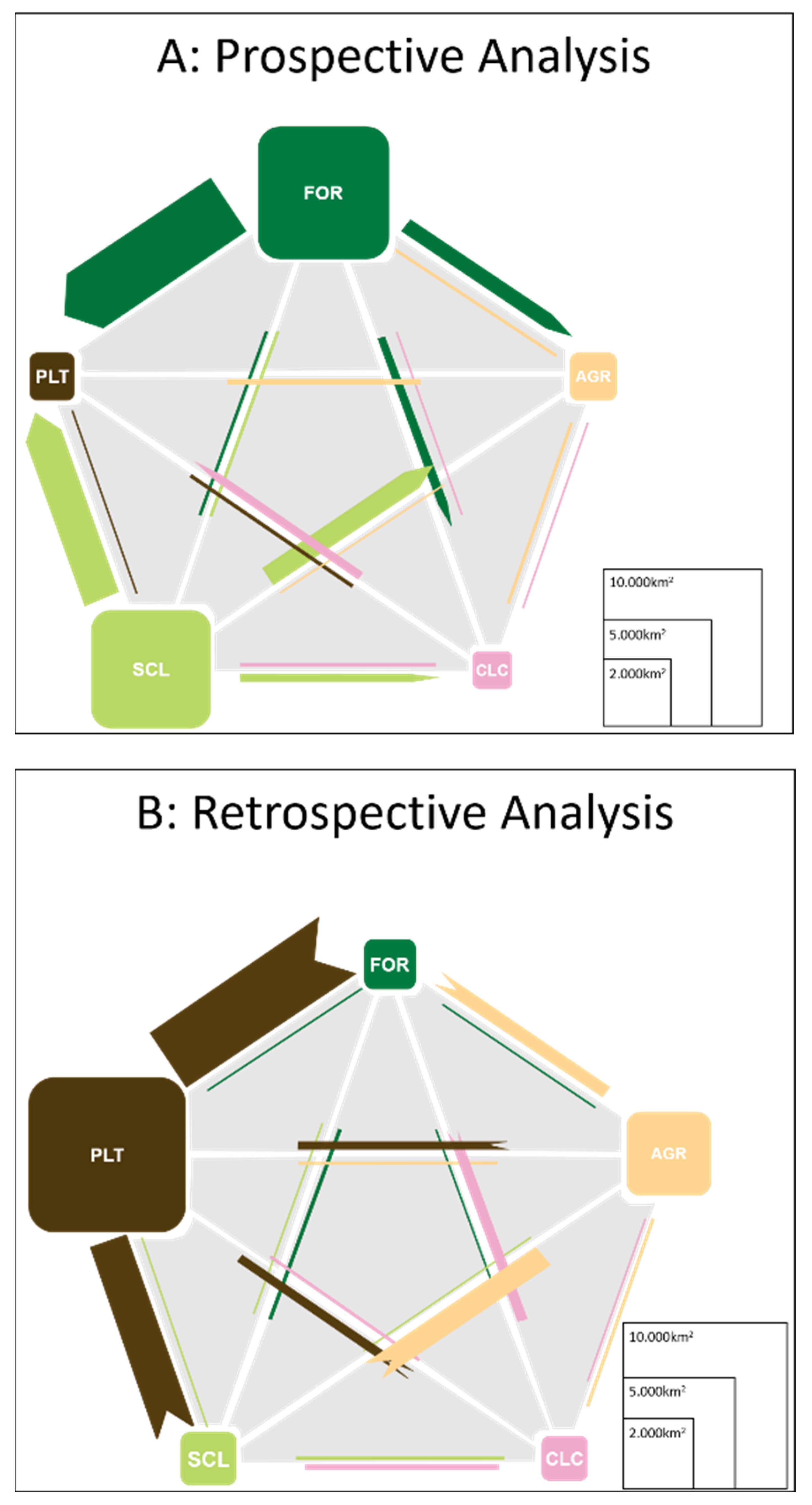
Figure 6.
Prospective analysis in five-year intervals focusing on forests. The percentages show which land use systems forests lost during the interval have been converted.
Figure 6.
Prospective analysis in five-year intervals focusing on forests. The percentages show which land use systems forests lost during the interval have been converted.

Figure 7.
Indirect analysis in five plus five-year intervals. Analysis shows the percentage of forests converted into the first five-year interval and the final land use system after 10 years.
Figure 7.
Indirect analysis in five plus five-year intervals. Analysis shows the percentage of forests converted into the first five-year interval and the final land use system after 10 years.
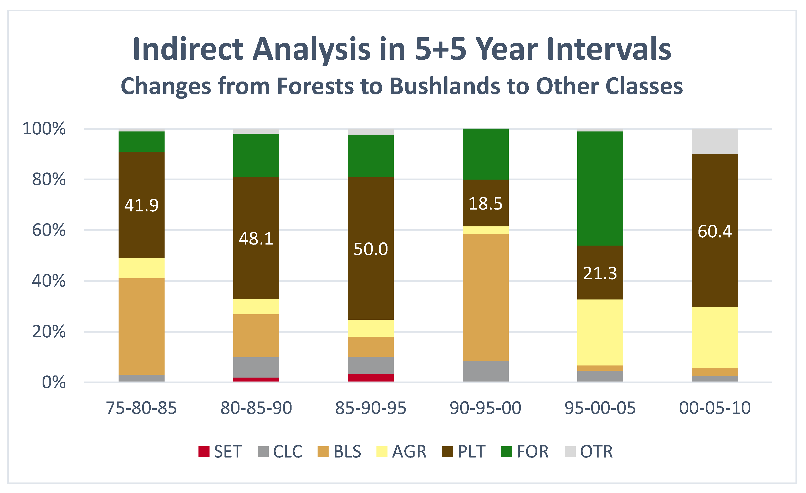
Figure 8.
Retrospective analysis in five-year intervals focusing on plantations. Percentages show from which land use systems plantations have been established.
Figure 8.
Retrospective analysis in five-year intervals focusing on plantations. Percentages show from which land use systems plantations have been established.
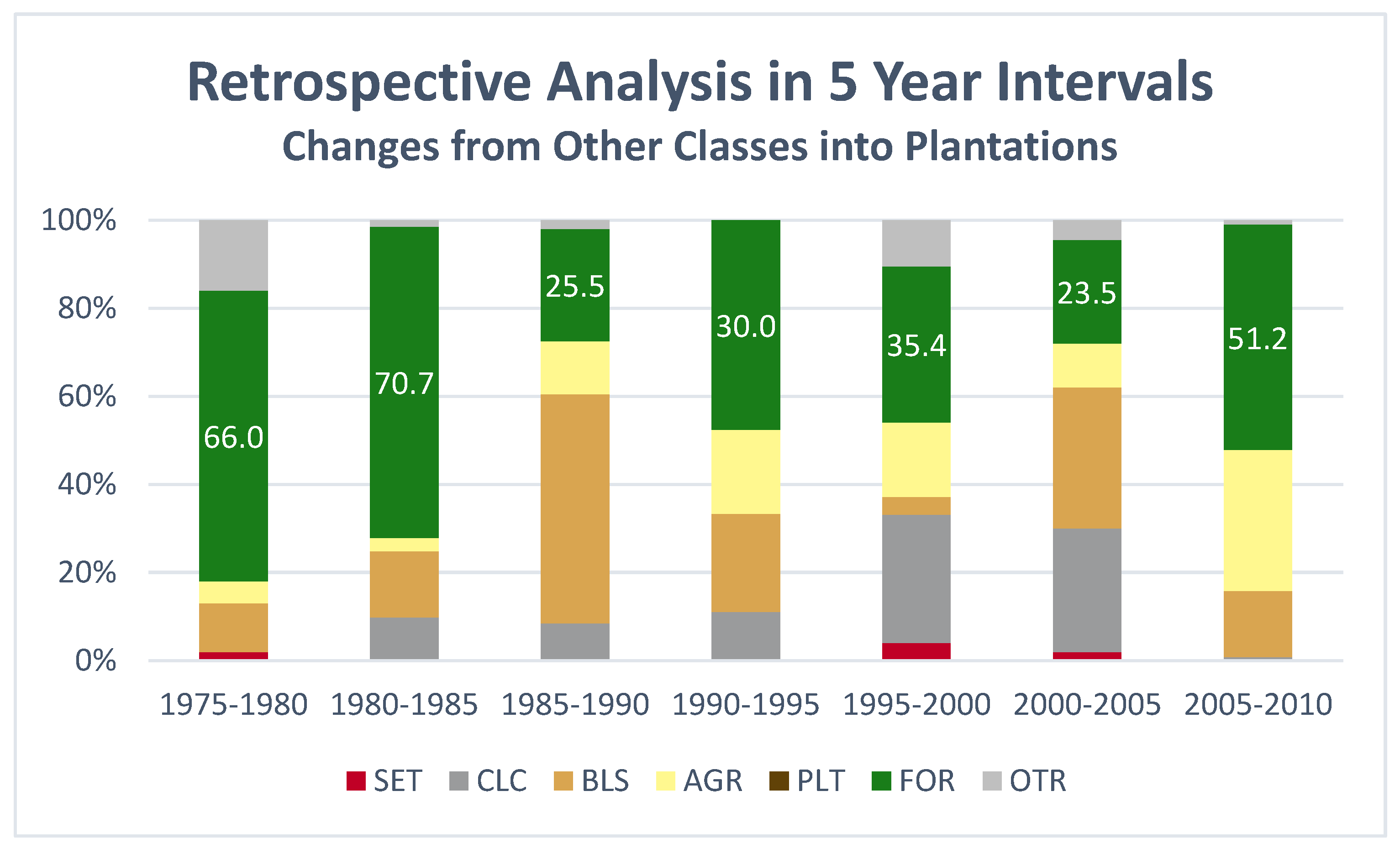

Table 1.
Main classes, abbreviations, and class colors used in classification. For a list of subclasses and class agglomeration, see Appendix B and Appendix C.
Table 1.
Main classes, abbreviations, and class colors used in classification. For a list of subclasses and class agglomeration, see Appendix B and Appendix C.
| Image Class | Name | Abbreviation | Class Color |
|---|---|---|---|
| 1 | Near-natural forests | FOR | |
| 2 | Tree plantations | PLT | |
| 3 | Agriculture | AGR | |
| 4 | Bushlands | BLS | |
| 5 | Clearcut | CLC | |
| 6 | Urban Areas | SET | |
| 7 | Waters | WAT | |
| 8 | Open Soils | OPS |
Table 2.
Accuracy values of land-use maps. Impr.: Improvement over standard approach (SVM on spectral data), OAA: Overall Accuracy, OSA: Overall Accuracy of standard approach, κ: Kappa coeff., minPA: lowest producer accuracy yielded (with class), minUA: lowest user accuracy yielder (with class). Class abbreviations, see Table 1.
| Year | Data | Impr. | OAA | OSA | κ | minPA | minUA |
|---|---|---|---|---|---|---|---|
| 2010 | TM | 13.4 | 96.2 | 82.7 | 0.96 | 81.4 SET | 82.4 OPS |
| 2005 | TM | 1.6 | 85.6 | 84.1 | 0.80 | 66.1 SET | 33.3 AGR |
| 2000 | ETM+ | 7.7 | 97.8 | 90.1 | 0.96 | 77.7 SET | 93.2 WAT |
| 1995 | TM | 6.8 | 96.7 | 89.0 | 0.97 | 82.3 CLC | 91.2 WAT |
| 1990 | TM | 2.8 | 91.1 | 88.3 | 0.88 | 57.2 AGR | 40.7 BLS |
| 1985 | TM | 15.1 | 95.5 | 80.3 | 0.93 | 80.4 AGR | 63.0 WAT |
| 1980 | MSS | 6.0 | 92.8 | 86.8 | 0.90 | 27.8 CLC | 43.89 BLS |
| 1975 | MSS | 7.8 | 78.2 | 70.4 | 0.72 | 40.7 CLC | 59.2 FOR |
Publisher’s Note: MDPI stays neutral with regard to jurisdictional claims in published maps and institutional affiliations. |
© 2022 by the author. Licensee MDPI, Basel, Switzerland. This article is an open access article distributed under the terms and conditions of the Creative Commons Attribution (CC BY) license (https://creativecommons.org/licenses/by/4.0/).
Share and Cite
MDPI and ACS Style
Braun, A.C. Deforestation by Afforestation: Land Use Change in the Coastal Range of Chile. Remote Sens. 2022, 14, 1686. https://doi.org/10.3390/rs14071686
AMA Style
Braun AC. Deforestation by Afforestation: Land Use Change in the Coastal Range of Chile. Remote Sensing. 2022; 14(7):1686. https://doi.org/10.3390/rs14071686
Chicago/Turabian StyleBraun, Andreas C. 2022. "Deforestation by Afforestation: Land Use Change in the Coastal Range of Chile" Remote Sensing 14, no. 7: 1686. https://doi.org/10.3390/rs14071686
Note that from the first issue of 2016, this journal uses article numbers instead of page numbers. See further details here.