Article

On the Potential for Remote Observations of Coastal Morphodynamics from Surf-Cameras

by
Matthew P. Conlin
1,*,
Peter N. Adams
1 and
Margaret L. Palmsten
2
1
Department of Geological Sciences, University of Florida, Gainesville, FL 32611, USA
2
U.S. Geological Survey, St. Petersburg Coastal and Marine Science Center, St. Petersburg, FL 33701, USA
*
Author to whom correspondence should be addressed.
Remote Sens. 2022, 14(7), 1706; https://doi.org/10.3390/rs14071706
Submission received: 5 February 2022 / Revised: 17 March 2022 / Accepted: 31 March 2022 / Published: 1 April 2022
(This article belongs to the Special Issue Remote Sensing Observation on Coastal Change)

Abstract

:
Recreational surf-cameras (surfcams) are ubiquitous along many coastlines, and yet are a largely untapped source of coastal morphodynamic observations. Surfcams offer broad spatial coverage and flexibility in data collection, but a method to remotely acquire ground control points (GCPs) and initial camera parameter approximations is necessary to better leverage this existing infrastructure to make quantitative measurements. This study examines the efficacy of remotely monitoring coastal morphodynamics from surfcams at two sites on the Atlantic coast of Florida, U.S.A., by leveraging freely available airborne lidar observations to acquire remote-GCPs and open-source web tools for camera parameter approximations, ignoring lens distortion. Intrinsic and extrinsic camera parameters are determined using a modified space resection procedure, wherein parameters are determined using iterative adjustment while fitting to remote-GCPs and initial camera parameter approximations derived from justified assumptions and Google Earth. This procedure is completed using the open-source Surf-Camera Remote Calibration Tool (SurfRCaT). The results indicate root mean squared horizontal reprojection errors at the two cameras of 3.43 m and 6.48 m. Only immobile hard structures such as piers, jetties, and boulders are suitable as remote-GCPs, and the spatial distribution of available points is a likely reason for the higher accuracy at one camera relative to the other. Additionally, lens distortion is not considered in this work. This is another important source of error and including it in the methodology is highlighted as a useful avenue for future work. Additional factors, such as initial camera parameter approximation accuracy, likely play a role as well. This work illustrates that, provided there is sufficient remote-GCP availability and small lens distortion, remote video monitoring of coastal areas with existing surfcams could provide a usable source of coastal morphodynamic observations. This is further explored with a shoreline change analysis from the higher-accuracy camera. It was found that only the largest (>6 m) magnitude shoreline changes exceed the observational uncertainty driven by shoreline mapping error and reprojection error, indicating that remotely calibrated surfcams can provide observations of seasonal or storm-driven signals.

Graphical Abstract

1. Introduction

Coastal morphodynamics occur over a range of time and space scales. For example, nearshore sandbars of length scales O (1–100 m) can migrate in the cross-shore direction meters to tens of meters per day in response to wave-generated bottom currents and short wave asymmetry [1,2,3]. Alternatively, convergent longshore sediment transport gradients created by complex inner-shelf bathymetry can drive the development and maintenance of cape features that are tens of kilometers in length over years to decades [4,5]. This array of process scales creates a well-established challenge to the study of coastal systems: a technique that is useful to observe coastal morphodynamics at one scale may not prove feasible at another [6,7,8,9,10]. As a result, many techniques have been developed to observe coastal morphodynamics in the field, each optimal for application over a finite range of time and space scales [11].
Video monitoring via fixed, shore-based camera stations is widely used by coastal researchers to obtain morphodynamic observations. The coastal zone presents many optical signals that can be linked to morphodynamic processes through established photogrammetric and computer vision techniques [12,13]. Further, fixed camera stations offer near-continuous daylight observations at a high spatial resolution over several kilometers at low cost, providing a valuable source of morphodynamic data. Coastal video monitoring has helped strengthen the understanding of many processes and parameters, including, among others: sandbar and shoreline behavior over a range of timescales [7,14,15], nearshore wave transformation and dissipation [16,17], and swash characteristics [18]. Both Splinter et al. [8] and Andriolo et al. [19] provide detailed reviews of coastal video monitoring applications that have been established to date.
Quantitative observations in the studies described above require projective mapping between image coordinates and real-world coordinates. The projection requires information about the parameters describing the camera and lens as well as information about the camera position and rotation. The information is typically found by identifying the real-world location of objects, called ground control points (GCPs) and the corresponding image coordinates of GCPs. Camera and lens information are often found in a separate step from camera position and rotation, although all information is determined using a least-squares fit.
Recently, researchers have developed methods to perform video monitoring with existing coastal video cameras deployed for recreational purposes (surf-cameras or surfcams). Surfcams provide a continuous stream of video data without the need for camera station equipment or installation and exist at many more beaches than research-grade imaging stations, where projective mapping between the image- and world-coordinates is known [19,20]. However, surfcams were not deployed for scientific aims. Therefore, surfcams are not usually optimized for morphodynamic studies, and special considerations must be made regarding their use. Mole et al. [21] and Bracs et al. [22] were among the first to explore the use of surfcams to quantitatively monitor coastal changes, each using commercial surfcams and software in Australia to monitor shoreline change with reasonable accuracy. Valentini et al. [23] utilized a commercial surfcam in France to reconstruct inter- and sub-tidal bathymetry with errors below 0.5 m. Finally, Andriolo et al. [19] applied the C-Pro Matlab tool developed by Sánchez-Garcia et al. [24] to a surfcam in Portugal, finding that surfcam images could be transformed to real-world space (geo-rectified) with errors generally below 2 m. Each of these later studies reported errors that are similar to those from traditional fixed camera stations.
Similar to traditional coastal video monitoring studies, nearly all applications of surfcams for coastal monitoring have relied on in situ observations of GCPs and intrinsic/extrinsic camera parameters (location, viewing angles). The fact that surfcams exist in many places throughout the world, and their web-streaming imagery can be accessed from anywhere, presents an opportunity to study beaches far from a researcher’s physical work location in near real-time without field costs. However, site visit requirements largely preclude this opportunity. Thus, a method to remotely obtain the necessary information to transform between image and real-world coordinates could be useful to unlock surfcams’ potential for coastal morphodynamic studies. Andriolo et al. [19] present the first and only remote use of a surfcam for morphodynamic observations. They use freely available web tools (Google Earth) to obtain initial camera parameter approximations and GCP locations, and the C-Pro software tool to complete the space resection procedure [24] to robustly transform image coordinates to real-world coordinates, despite uncertainties in the observations. They report median reprojection errors below 3 m for the technique, although some checkpoints obtained residuals on the order of 10 m or more. However, their approach to obtaining estimates of GCP elevation relies on the application of shoreline position and water level models to create an intertidal bathymetry map from the imagery collected over the course of a tidal cycle, with the GCP elevations interpolated from this map. This procedure prevents the use of GCPs outside of the intertidal zone, presenting a major limitation to the transferability of the method to other locations, which may be micro-tidal and/or contain candidate GCPs outside this relatively narrow zone.
In this study, we examine the feasibility of a more general method to remotely use surfcams for morphodynamic observations that utilizes freely available airborne lidar observations to identify GCPs. Remote-GCPs derived from the lidar data are used alongside initial camera parameter approximations derived from Google Earth in a modified space resection procedure to remotely geo-rectify images from two surfcams on the Atlantic coast of Florida, U.S.A. This procedure is facilitated by the open-source Surf-Camera Remote Calibration Tool (SurfRCaT), which provides these capabilities in a self-contained, graphical user-interface-driven software application [25].

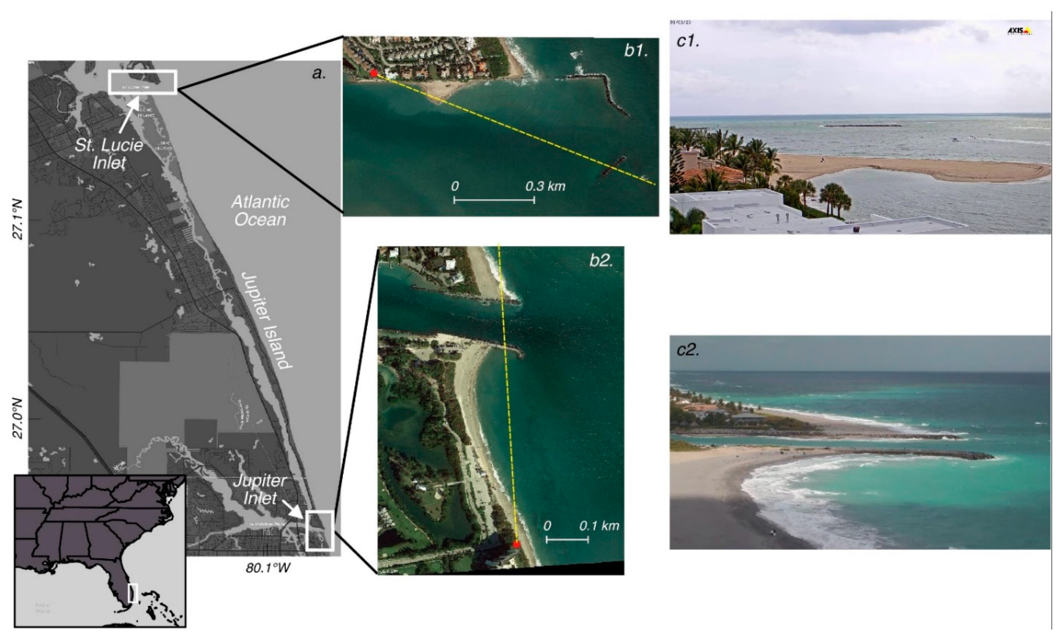
2. Study Sites and Surfcams

The surfcams used in this work are located at the north and south ends, respectively, of Jupiter Island, a 25-km-long barrier island on the Atlantic coast of Florida (Figure 1). The northern camera overlooks a portion of St. Lucie Inlet (Figure 1a,b1,c1), and will be referred to hereafter as the St. Lucie camera, whereas the southern camera overlooks Jupiter Inlet (Figure 1a,b2,c2), and will be referred to hereafter as the Jupiter camera. Jupiter Island lies in a microtidal setting (mean tidal range < 1 m). Analysis of wave observations since 2006 from the nearest buoy, located 44 km to the northnorthwest of St. Lucie Inlet in 16.2 m depth, indicates an average significant wave height of 0.96 m and period of 7.39 s [26]. The 98th percentile significant wave height and wave period from this record are 2.18 m and 10.22 s.
The St. Lucie camera is situated atop a condominium building at an elevation of ~20 m (NAVD88). A sand spit within the camera’s field-of-view periodically forms inside the atypically shaped jetties/breakwaters at the mouth of the inlet (Figure 1). The spit exists because the northern jetty was designed as a “weir-jetty” such that prevailing southward longshore currents transport sediment through the weir, allowing sand to accumulate inside the inlet mouth as a spit [27]. The spit is monitored and regularly dredged by the U.S. Army Corps of Engineers.
The Jupiter camera is situated atop a condominium building at an elevation of ~45 m (NAVD88). This camera is a pan-tilt-zoom (PTZ) camera, cycling between four unique views with a dwell of approximately 30 s at each. The camera overlooks an embayed beach adjacent to the Jupiter Inlet south jetty, and a short stretch of beach adjacent to the north jetty (Figure 1b2,c2). Jupiter Inlet is heavily managed, and the beach adjacent to the south jetty is chronically erosive due to sediment starvation [28]. As such, beach nourishments here are relatively frequent: a total of 26 nourishments have been completed since 1957, with the most recent at the time of writing in 2020 [29].
Both cameras continuously capture and livestream video to the web [30,31] at a resolution of 1080 × 1920 pixels. Partnerships with the owners/operators of the cameras facilitated access to them and their web-streaming imagery.

3. Materials and Methods

3.1. Video Acquisition

After obtaining permission from the camera owners/operators, Python scripts were created to download web-streaming imagery. Videos were obtained concurrently with in situ measurements of GCPs (see Section 3.3) on 3 March 2020 for the St Lucie camera and 2 March 2020 for the Jupiter camera. Video from both cameras was acquired at 30 frames per second, and still images were extracted for remote-GCP identification and subsequent photogrammetric transformation.

3.2. Photogrammetric Transformations

3.2.1. Modified Space Resection

The relationship between a three-dimensional point on Earth and an image capturing that point is described by the collinearity conditions:
x = x 0 f ( m 11 ( X A X L ) + m 12 ( Y A Y L ) + m 13 ( Z A Z L ) m 31 ( X A X L ) + m 32 ( Y A Y L ) + m 33 ( Z A Z L ) )
y = y 0 f ( m 21 ( X A X L ) + m 22 ( Y A Y L ) + m 23 ( Z A Z L ) m 31 ( X A X L ) + m 32 ( Y A Y L ) + m 33 ( Z A Z L ) )
where ( x , y ) are the image coordinates of the point, ( X A , Y A , Z A ) are the real-world coordinates of the point, ( X L , Y L , Z L ) are the real-world coordinates of the camera sensor, ( x 0 , y 0 ) are the principal point coordinates of the image, f is the calibrated principal distance (focal length) of the camera, and m i j are the elements of the image-space to object-space rotation matrix composed of three rotation angles ( ω , ϕ , κ ) .
The collinearity conditions contain nine parameters associated with the camera ( X L , Y L , Z L , ω , ϕ , κ , f , x 0 , y 0 ) , which, once determined, allow for conversion between image space and real-world coordinates (geo-rectification). The process of space resection involves determining the extrinsic camera parameters ( X L , Y L , Z L , ω , ϕ , κ ) based on GCP observations, a lab calibration to determine the intrinsic parameters ( f , x 0 , y 0 ) , and an initial approximation of each extrinsic parameter. Initial approximations for each of the extrinsic parameters are iteratively adjusted to converge on optimal values in terms of the reprojection error at the GCPs. Space resection is well documented, and the reader is referred to Wolf et al. [32] for more information.
Since surfcams are already deployed, performing lab-calibrations to determine intrinsic camera parameters is not possible (and doing so would undermine the goal of a fully remote workflow). Thus, a modification to the traditional space resection procedure is required. In this work, the three intrinsic parameters are included alongside the extrinsic parameters in the iterative adjustment. The space resection problem is, therefore, expanded to:
[ F 1 ω F 1 ϕ F 1 κ F 1 X L F 1 Y L F 1 Z L F 1 f F 1 x 0 F 1 y 0 G 1 ω G 1 ϕ G 1 κ G 1 X L G 1 Y L G 1 Z L G 1 f G 1 x 0 G 1 y 0 F n ω F n ϕ F n κ F n X L F n Y L F n Z L F n f F n x 0 F n y 0 G n ω G n ϕ G n κ G n X L G n Y L G n Z L G n f G n x 0 G n y 0 ] [ d ω d ϕ d κ d X L d Y L d Z L d f d x 0 d y 0 ] = [ x 1 ( x 0 f r q ) y 1 ( y 0 f s q ) x n ( x 0 f r q ) y n ( y 0 f s q ) ] + [ V x 1 V y 1 V x n V y n ]
where F and G denote Equations (1) and (2), respectively, evaluated at the current approximations of all unknown parameters; ( d ω , d ϕ , d κ , d X L , d Y L , d Z L , d f , d x 0 , d y 0 ) are corrections to each parameter; r is the numerator of the fraction in Equation (1); s is the numerator of the fraction in Equation (2); q is the denominator of Equations (1) and (2); subscript n denotes GCP number, and ( V x n , V y n ) are the x and y residuals for GCP n .
With nine parameters in the photogrammetric transformation (Equation (3)), the procedure outlined above requires observations of at least five GCPs. Furthermore, correlations may exist between extrinsic and intrinsic camera parameters; for example, a change in Z L can be nearly perfectly compensated for by a change in f . A new two-step solution methodology was developed to overcome potential correlations between intrinsic and extrinsic parameters. In this approach, only a subset of the nine parameters are free to adjust during each step. In the first step, the three rotation angles ( ω , ϕ , κ ) and three camera intrinsic parameters ( f , x 0 , y 0 ) are free to adjust, while camera location parameters ( X L , Y L , Z L ) remain fixed at their initial approximations. Then, the adjusted values for the six free parameters in step one are used as initial approximations for step two, where only ( X L , Y L , Z L ) are free to adjust. This approach has the additional benefit of creating no more than six unknown parameters for either step, allowing the solution to be determined with as few as three GCPs. Andriolo et al. [19] effectively used a similar two-step solution approach for photogrammetric transformations of surfcam images. Note that this technique does not account for lens distortion.

3.2.2. Remote-GCP and Camera Parameter Extraction

The space resection process relies on initial approximations of the nine camera parameters. Initial approximations for some camera parameters were obtained via Google Earth. The location of each camera ( X L , Y L ) and the azimuth viewing angle (used later along with assumptions of camera tilt and swing viewing angles to derive approximations for ω , ϕ , κ ; [32]) were extracted directly from Google Earth. As elevations reported from Google Earth are unreliable [19], the elevation of the cameras ( Z L ) was extracted from Google Earth by counting the number of stories of the buildings atop which the cameras sit from available imagery, assuming a height of 4.27 m (14 feet) per story and that the base of the buildings is at 0 m elevation. Initial approximations for the remaining parameters were obtained with reasonable assumptions, as follows. Camera tilt, measured up from nadir, and swing, measured counterclockwise from horizontal, was estimated as 80° and 180° (i.e., no swing), respectively, which appears to be reasonable after an examination of images from many surfcams. Initial approximations for the principal point coordinates ( x 0 , y 0 ) were taken as the center of the image. An initial approximation for the focal length ( f ) was obtained through a geometric consideration of the pinhole camera model as:
  f = W 2 t a n ( α 2 )
where W is the width of the camera sensor (taken as the width of the image) and α is the camera’s horizontal field of view. We assumed α = 60 ° based on other known webcams used for environmental applications [21,22,33,34], although this could also be estimated based on the method of e.g., [35].
GCPs were extracted remotely using freely available airborne lidar data. For each camera, publicly available datasets from the National Oceanic and Atmospheric Administration [36] were parsed to find those that covered the estimated location ( X L , Y L ) of the camera. Datasets not covering the U.S. state and coast of the camera locations were removed. The remaining datasets were then examined to determine their spatial coverage by querying the file describing the geographic extent of the dataset. For each camera, an applicable dataset was chosen, and data within an angular distance of ± 20 ° of the assumed azimuthal direction and within 500 m range of the camera were downloaded. Dataset 8950 (collected in 2018) was chosen for the St. Lucie camera, and dataset 6330 (collected in 2017) for the Jupiter camera. Features that were visible in both the lidar point cloud and an image from the camera were then identified as remote-GCPs by manually selecting them in both datasets (Figure 2).
The remote-GCP extraction and modified space resection procedures were conducted using SurfRCaT. SurfRCaT facilitates downloading lidar data and remote-GCP matching for any surfcam of interest through a graphical user interface-driven software application [25]. An image from each camera was then geo-rectified to real-world coordinates using the adjusted camera parameter values from the modified space resection.

3.3. Accuracy Assessment of Photogrammetric Transformations

The accuracy of the transformation from image space to real-world coordinates was assessed using points surveyed with real-time kinematic (RTK) GPS within the field of view of the cameras. A 1.2 × 1.2 m wooden board was painted with a 2 × 2 black and white checkerboard pattern and moved to various locations within the fields of view of the cameras for this purpose. The center of the checkerboard was surveyed at each location and subsequently identified in the image. Checkpoints were surveyed on the same day as the images used for geo-rectification were collected, and camera locations were also surveyed at this time. Remote-GCPs were not surveyed with GPS. The reprojected position of each surveyed point was obtained by solving Equations (1) and (2) for the ( X A , Y A ) real-world locations of the points given their digitized image coordinates ( x , y ) , the adjusted camera parameter values from the space resection, and the measured real-world elevation Z A of the points. The reprojected positions were compared with surveyed positions to determine reprojection errors at each point (Euclidean distance), and accuracy statistics such as the root-mean squared (RMS) reprojection error were derived.

4. Results

The reprojection residuals at surveyed points arising from the modified space resection procedure at both cameras are shown atop geo-rectified images in Figure 3. For the 32 surveyed checkpoints at the St. Lucie camera (Figure 3a), the median reprojection residual is 2.65 m, the mean residual is 2.92 m and the root mean squared (RMS) residual is 3.43 m. All points obtained residuals below 10 m, and 28 of the 32 checkpoints (88%) obtained residuals below 5 m; all those that did not are on the north-eastern edge of the spit. The highest accuracy is found near the center of the image and spit, with accuracy degrading away from this site in both longshore directions, although more so to the east (Figure 3a). Residuals are dominated by error in the along-range direction (approximately east-west in this case), rather than the cross-range direction (Figure 3a, inset).
At the Jupiter camera (Figure 3b), the median reprojection residual is 5.32 m, the mean residual is 5.70 m and the RMS residual is 6.48 m. 35 of the 38 points (92%) obtained residuals below 10 m, while 15 (39%) obtained residuals below 5 m. In general, the calibration is most accurate for points in the middle of the alongshore region sampled by the image, between ~300 and 500 m relative Northing, especially along the inland edge of this region (Figure 3b). Two of the three southernmost checkpoints obtained residuals above 10 m (15.91 m for the easternmost point and 11.54 m for the westernmost point), indicating that this portion of the geo-rectified product is of relatively low accuracy. The third checkpoint with a residual >10 m is found in the central portion of the geo-rectified image (Figure 3b); the residual at this point is 11.06 m. As with the St. Lucie camera, residuals are dominated by error in the along-range direction (approximately northsouth in this case) rather than the cross-range direction (Figure 3b, inset).
The initial approximations and final adjusted values for the camera parameters at each camera are shown in Table 1. At both cameras, final values of camera location and elevation ( X L , Y L , Z L ) differ from initial approximations by <1 m, and look angles ω and κ differ by <25°. However, at both cameras, the final values of ϕ are >180° different from the initial approximations. This is equivalent to similar tilt and swing values, but final azimuth values >180° different from initial approximations (Table 1). Additionally, at both cameras, the final value for the focal length ( f ) is about twice that of the initial approximation. At the St. Lucie camera, the final values for the principal point coordinates ( x 0 , y 0 ) differ by ~100–200 pixels from initial approximations. At the Jupiter camera, the principal point coordinates differ by ~500–1000 pixels and the final values are negative. The fact that reasonable projections are obtained with final camera parameter values that may differ substantially from initial approximations is discussed in Section 5.1.

5. Discussion

The fully remote photogrammetric transformations produced RMS errors of 3.43 m and 6.48 m and median values of 2.65 and 5.32 m at the St. Lucie and Jupiter cameras, respectively. These values are similar to the median error in the remote approach of Andriolo et al. [19] of 2.2 m, particularly at the St. Lucie camera. As a comparison, satellite images from the Landsat mission, which have recently become a widely used source of shoreline change observations, are considered to have valid geometric accuracy when RMS errors are <12 m [37].
Accuracy differences between the two cameras, in the context of differences between them, could shed light on important considerations for fully remote applications of surfcams for coastal morphodynamic measurements. Below, we investigate possible sources of error at each camera, and illustrate the possible utility of the fully remote method through a case study of the shoreline changes derived from the St. Lucie camera.

5.1. Sources of Error

Lens distortion has not been accounted for in the present study, and this is likely a contributing factor to the observed reprojection errors. At both cameras, the adjusted camera parameter values resulted in regions of maximum accuracy. For the St. Lucie camera, the maximum accuracy zone is in the region at the center of the image, whereas for the Jupiter camera, it is in the region at the edge of the image (Figure 2 and Figure 3). Accuracy degrading away from the center of the image is consistent with the typical pattern of lens distortion, which is also at a minimum in the center of the image. This suggests that not accounting for lens distortion could contribute to reprojection error at the edges of the image at the St. Lucie camera, but not at the Jupiter camera. This may be because the lens of the Jupiter camera produces less distortion than the lens of the St. Lucie camera, although this is not visibly apparent. Given that both of the cameras have low distortion (e.g., relatively straight horizon lines, Figure 1) but may have reprojection errors due to distortion, accounting for this parameter may be critical for surfcams that use higher distortion lenses. In the work of Sánchez-Garcia et al. [24], photogrammetric transformations of surfcam images are made that account for lens distortion by using the empirical inverse model for compensating lens distortion outlined by [38]. A similar approach could be incorporated into SurfRCaT, and this is a prudent direction for future research in order to increase the applicability of the tool. Distortion coefficients could also be estimated based on the deviation from a straight line of the visible horizon, e.g., [39], and this is the subject of ongoing work.
An important parameter in determining the accuracy of photogrammetric transformations is GCP selection. For photogrammetric applications it is generally ideal to identify many GCPs, covering the entire image format [32,40,41]. However, this may not be feasible when remotely identifying GCPs with airborne lidar observations. Only features that do not change substantially over the timescale of years and that are easily identifiable in lidar observations, such as piers, jetties, buildings, and/or boulders, can be used as remote-GCPs. Years may separate the available lidar observations from the surfcam image being used; the two lidar datasets used in this study were collected two and three years before the images from the St. Lucie and Jupiter cameras were acquired, respectively. The identification of small-scale features near or below the spatial resolution of airborne lidar observations (typically on the order of 1 pt/m2) can also pose a challenge. For example, while a jetty likely meets the requirement of temporal stability, it is difficult to co-identify a precise point on the jetty in both the lidar data and the surfcam image due to spatial aliasing in either/both datasets over the irregular surface of the jetty.
To illustrate these ideas, it is useful to consider that the two cameras present differences in remote-GCP availability. Features suitable to serve as GCPs (buildings, jetties) lie within an image region that covers only ~25% of the Jupiter camera image format. In contrast, suitable GCPs cover ~50% of the St. Lucie camera image (see Figure 2). At both cameras, a total of five GCPs were used, with two identified on jetties and the rest representing building corners. As can be observed from Figure 2, the co-identification of precise points on the jetties was not possible. A best estimate was used, which likely contributed to the observed reprojection errors. Ideally, only objects such as building corners, where more precise positions can be obtained, should be used, although GCP distribution is of the upmost importance, hence our decision to use jetties here. The fact that reprojection errors are lower at the St. Lucie camera could indicate that remote-GCP availability and distribution in the image is a primary limiting factor in acquiring fully remote morphodynamic observations from surfcams. Indeed, the fact that surfcam images often contain large areas (e.g., water, sky) without candidate GCPs reflects this limitation, as this remote approach is not applicable in locations that entirely lack structures suitable to serve as remote-GCPs.
Initial camera parameter approximations may also be a factor influencing the lower reprojection errors at the St. Lucie camera. Site measurements via RTK GPS reveal that our initial extrinsic camera parameter estimates, which we derived from Google Earth, were closer to true values at the St. Lucie camera than at the Jupiter camera. For example, initial estimates for camera location/elevation differed from the surveyed location by 18.5 m in the horizontal and 19.3 m in the vertical at the Jupiter camera and 9.1 m in the horizontal and 1.2 m in the vertical at the St. Lucie camera. While this indicates a limitation in the use of Google Earth to obtain initial approximations, especially to estimate Z L , it also likely illustrates the established idea that better initial approximations often lead to higher-accuracy transformations because they reduce the likelihood of convergence on a (potentially suboptimal) local reprojection error minimum [32,42]. Difficulties in remotely obtaining initial approximations is an additional limiting factor in fully remote applications of surfcams. Theoretically, airborne lidar observations, rather than Google Earth, could be used to derive more accurate ( X L , Y L , Z L ) approximations, and future studies could incorporate this method. Additionally, Sánchez-Garcia et al. [24] present a method to obtain initial approximations for camera view angles ( ω , ϕ , κ ) using the horizon, and this method could be incorporated in future work to reduce errors. Finally, using a direct linear transform (DLT) approach [43] could produce initial approximations without remote measurements of camera parameters [24]. This closed-form approach, however, is known to be limited in terms of accuracy [44].
Due to the potential for limited remote-GCP distribution and potential errors in remotely derived initial approximations, our modified space resection utilizes an unbounded adjustment of all parameters. This effectively compensates for errors in the inputs by allowing the adjustment to converge to a local minimum in terms of reprojection error, creating reasonable reprojections despite poor initial parameter estimates that may prevent convergence on a global minimum [42]. This is shown in Figure 4, where the collinear geometry created by both the initial camera parameter approximations and final adjusted values are compared at each camera. Figure 4 illustrates that position of object projections using the final adjusted values are similar to those obtained using initial approximations, despite final values that sometimes substantially differ from initial approximations, such as the negative principal point coordinates at the Jupiter camera (Table 1). It is also worth noting that Equations (1) and (2) are equally valid for an image plane located in front of or behind the camera; hence the ~180 ° difference between azimuth initial approximations and final values. This method stands in contrast to traditional coastal video-imaging techniques, where all camera parameters are precisely measured or solved [12]. However, the method is comparable to Structure from Motion (SfM) techniques, where camera parameter values generally only matter for the generation of a reasonable reprojection [42].

5.2. Shoreline Change Case Study

To further explore the potential utility of remotely using surfcams to study coastal morphodynamics, a shoreline change study was undertaken using observations from the higher-accuracy St. Lucie camera. Morphodynamic studies using traditional fixed camera stations do not typically report or discuss the observational uncertainty stemming from the photogrammetric transformation from image to real-world coordinates. Instead, observational error in the derived shoreline change is assessed by comparing video-derived observations to those of a high-accuracy, in situ technique such as RTK GPS [7,11,45]. These studies note that video-derived shoreline observation uncertainties stem from (1) error in the (typically automated) identification of shoreline position and (2) error in the estimated elevation of the shoreline derived from a water-level model (ranging in complexity from tidal elevation only to detailed two-dimensional hydrodynamic modeling). We will refer to these sources of error in combination as shoreline mapping error. However, observational uncertainty is also partly due to errors in the photogrammetric transformation (reprojection error). The detailed photogrammetric methods underpinning the Argus program are described in detail in Holland et al. [12], and they report reprojection errors of just a few centimeters for fixed camera stations. Hence, this is likely only a small source of uncertainty relative to those described above. However, for remote transformations of surfcams, such as those described herein, reprojection errors are much larger (order meters, in this work) due to the factors described in Section 5.1, and thus cannot be neglected.
In this case study, we will consider shoreline position change observations along the spit within the field of view of the St. Lucie camera in the context of uncertainty driven by both shoreline mapping error and reprojection error. The spit (Figure 1c1) is unique in that its existence is due to anthropogenic engineering of the inlet to create a weir jetty system [46]. In addition to the video downloaded in March, videos were downloaded from the St. Lucie camera on most days in May and 1 August 2020. Every collected video was sub-sampled to a frame rate of 1 Hz, and, for each video, all frames were averaged to create a time-exposure image (timex). Each timex was geo-rectified to a planimetric map using the adjusted camera parameter values given in Table 1 and a local camera-centered coordinate system with x in the eastwest direction and y in the northsouth direction. Timex images were geo-rectified to the mean water level at the initiation of video collection as interpolated from the two closest NOAA water level stations: Trident Pier (station 8721604), 150 km to the north; and Lake Worth Pier (station 8722670), 75 km to the south. Water-level differences at the two stations were always less than 0.23 m. The shoreline position on each timex was identified using the color channel divergence (CCD) technique described in Plant et al. [45] and implemented in Harley [47]. Mapped shorelines were then corrected for observed tidal elevation using the linear slope-based correction neglecting wave setup described in Vos et al. [37], assuming a 1:10 cross-shore slope for the entire feature. Visual field evidence confirms a steep slope along the feature, though this was not directly measured. Water-level-corrected shorelines were then intersected with two cross-shore transects placed on the seaward side of the spit using the method in Vos et al. [48] to yield cross-shore shoreline position change time series at both transects.
We consider uncertainty in these shoreline change observations stemming from both shoreline mapping error and reprojection error at the camera. Plant et al. [45] found horizontal error in shoreline position observations derived from the CCD method to be comparable to those of other methods, which have been documented at 5.1 m [7]. The reprojection error is taken as the RMS value at the St. Lucie camera of 3.43 m. We derived total shoreline observation uncertainty by adding these two sources in quadrature, resulting in an observational uncertainty estimate of 6.1 m.
CCD-derived shorelines are shown in Figure 5. Observations on 5 March and 1 May reveal a clockwise rotation and lateral extension of the spit over this two-month period, with the head of the spit migrating westward out of the field of view of the camera (Figure 5). The visible portion of the spit remained relatively stable throughout May, with the most noticeable variability being in the sinuosity of the spit’s seaward (southern) edge (Figure 5). Changes between 31 May and 1 August are relatively qualitatively small compared to those between 5 March and 1 May, with a near disappearance of sinuosity along the spit’s seaward edge (Figure 5).
Harley et al. [11] and Vos et al. [37] use the semivariogram as a method of quantitatively assessing the typical timescales of variability in a shoreline signal relative to uncertainty in the observational technique. While we do not have the necessary data to quantify typical timescales of variability on this weir jetty spit with this method, we examined the observations of shoreline change over multiple timescales relative to the derived observational uncertainty. Figure 6 shows water-level-corrected shoreline position changes at the two transects shown in Figure 5 (red transects on image in the lower left corner) relative to uncertainty. This is shown for changes between every observation as well as end-point changes over each of the four weeks of near-daily observations in May. Figure 6 reveals that the largest magnitude shoreline changes at both transects—a 12 m retreat between 31 May and 1 August at the eastern transect and a nearly 36 m retreat between 5 March and 1 May at the western transect in response to the large-scale spit reorientation visible in Figure 5—are outside of uncertainty. However, none of the near-daily observations in May, as well as only one of the four weekly scale changes at the western transect and none at the eastern transect, are outside of uncertainty (Figure 6). Thus, the remotely calibrated surfcam produces observations that only have a useful precision for the largest magnitude shoreline changes. These large changes took place over timescales of 2–3 months.
Importantly, the observability of a morphodynamic signal from video imagery, as with any data collection technique, is a function of the magnitude of the signal in relation to observational uncertainty. Shoreline changes greater than the observational uncertainty reported here (6.2 m) have commonly been reported over a range of timescales, including as a result of storms [49,50,51,52], in response to seasonal variability in wave/water level forcing [53,54], and over interannual and longer timescales [4,11,55,56]. Thus, this case study illustrates that the method described here is useful for measuring large magnitude shoreline changes in response to storms or longer timescales, provided similar reprojection errors can be obtained as a function of lens distortion, remote-GCP availability, and initial camera parameter approximation accuracy.
Ultimately, this case study shows that the remote approach presented here could enable morphodynamic observations from a large and growing network of existing surfcams in the United States, provided there is sufficient remote-GCPs and small lens distortion. This could allow for targeted studies at a coastline of interest, no matter the location relative to the researcher’s physical work location, to take place relatively easily and without field costs. Such studies could be performed in other countries as well, provided surfcam images and open-source lidar data were available. While SurfRCaT was designed to interface with a large repository of existing lidar datasets covering the United States [25], the tool could be modified to utilize similar repositories from other countries, such as the Actueel Hoogtemodal Nederland (AHN) in the Netherlands [57] and that provided by the Terrestrial Ecosystem Research Network in Australia [58]. Such datasets may not be available everywhere; in their absence, SurfRCaT could be modified to allow for any point cloud file to be used, such as those collected via terrestrial lidar or structure from motion photogrammetry. Given that most surfcams are in developed locations, targeted studies utilizing the remote approach outlined here could focus on the morphodynamics of human-altered coastlines, an understudied environment [59]. Additionally, remote surfcam-based observations could provide validation for coastal change and coastal flood models [60] with unprecedented spatial coverage. More generally, shoreline observations from a variety of sites covering many coastal regions are necessary to garner a complete understanding of the impacts of a changing climate on coastlines; remote calibration could make surfcams a valuable and widely usable tool to obtain these.

6. Conclusions

This study examines the potential for remote observations of coastal morphodynamics from pre-existing recreational surf-cameras (surfcams) using the open-source Surf-camera Remote Calibration Tool (SurfRCaT). At two surfcams on the Atlantic coast of Florida, GCPs were remotely extracted using openly available airborne lidar observations. The remote-GCPs were used with initial camera parameter approximations derived from Google Earth in a modified space resection procedure that includes the intrinsic parameters and uses a two-step solution methodology to establish the relationship between image and real-world coordinates, not accounting for lens distortion. Root mean squared reprojection errors of 3.43 m and 6.48 m were observed at the two cameras. The final adjusted camera parameter values were similar to initial approximations for camera location and elevation, though they differed substantially for azimuth viewing angle and camera intrinsic parameters. The lower reprojection errors at one camera could be linked to multiple factors, including the fact that lens distortion was not accounted for. The inclusion of this parameter could be necessary for the use of highly distorted surfcams, and its inclusion in the methodology presented herein is a prudent direction for future research. The difference in errors could also be linked to the wider distribution of remote-GCPs at that site, covering 50% of the image as opposed to just 25% at the other camera. The difference illustrates the importance of remote-GCP availability. Finally, initial approximations of camera location/elevation are closer to the true values at the higher-accuracy camera, providing another possible explanation, although errors in initial parameter approximations are compensated for through an unbounded adjustment of all parameters in the modified space resection.
A case study of shoreline changes along a weir jetty spit derived from the higher-accuracy camera was used to further explore the potential for remote observations of coastal morphodynamics from surfcams. A comparison between shoreline change observations and the observational uncertainty derived from both shoreline mapping error and reprojection error illustrated that large-magnitude (>6 m) shoreline changes spanning 2–3 months were observable outside of uncertainty, although smaller magnitude dailyweekly scale changes were not. Given that the observability of morphodynamic signals is a function of the magnitude of the signal in relation to the observational uncertainty, this case study illustrates that surfcams could be used remotely to observe morphodynamic signals such as storm induced and seasonal shoreline changes. Given the high number of existing surfcams in the United States, and likely in other parts of the world, we conclude that, provided there are sufficient remote-GCPs and small lens distortion, the approach outlined here could unlock a sizable new source of morphodynamic observations for coastal researchers.

Author Contributions

Conceptualization, M.P.C.; methodology, M.P.C.; software, M.P.C.; validation, M.P.C.; formal analysis, M.P.C.; investigation, M.P.C., M.L.P. and P.N.A.; resources, P.N.A.; data curation, M.P.C.; writing—original draft preparation, M.P.C.; writing—review and editing, M.P.C., P.N.A. and M.L.P.; visualization, M.P.C.; supervision, P.N.A.; project administration, M.P.C.; funding acquisition, M.P.C., P.N.A. and M.L.P. All authors have read and agreed to the published version of the manuscript.

Funding

This research was supported by the University of Florida Graduate Research Fellowship, The Southeast Coastal Ocean Observing Regional Association through their annual Student Data Challenge in 2019, and the U.S. Army Corps of Engineers Engineering with Nature (EWN) Program (to P.N.A.). M.L.P. was funded by the U.S. Geological Survey (Coastal and Marine Hazards and Resources Program).

Institutional Review Board Statement

Not applicable.

Data Availability Statement

All analyses presented herein (including figures) can be recreated using the pyArgus_mpc Python package openly available on GitHub (https://github.com/conlin-matt/pyArgus_mpc; accessed on 31 March 2022). All necessary data and top-level script files to recreate analyses can be found in the appropriate subdirectories in pyArgus_mpc/SurfcamArgus/GeophysicalAnalyses. This is except for the St. Lucie inlet videos for the shoreline change analyses; these are openly available for download on figshare at https://doi.org/10.6084/m9.figshare.c.5816801.v1 (accessed on 31 March 2022). Installation instructions for the Python package can be found in the readme.

Acknowledgments

The authors wish to extend their gratitude to Joseph Chaison at the Jupiter Inlet District and Butch Bayley at the Sailfish Marina of Stuart for facilitating access to the cameras and their imagery. Many thanks to Jenna Brown for reviewing the manuscript. The authors also wish to thank four anonymous reviewers for providing useful feedback. Any use of trade, firm, or product names is for descriptive purposes only and does not imply endorsement by the U.S. government.

Conflicts of Interest

The authors declare no conflict of interest.

References

  1. Elgar, S.; Gallagher, E.L.; Guza, R.T. Nearshore sandbar migration. J. Geophys. Res. Ocean. 2001, 106, 11623–11627. [Google Scholar] [CrossRef]
  2. Hsu, T.J.; Elgar, S.; Guza, R.T. Wave-induced sediment transport and onshore sandbar migration. Coast. Eng. 2006, 53, 817–824. [Google Scholar] [CrossRef] [Green Version]
  3. Ruessink, B.G.; Pape, L.; Turner, I.L. Daily to interannual cross-shore sandbar migration: Observations from a multiple sandbar system. Cont. Shelf Res. 2009, 29, 1663–1677. [Google Scholar] [CrossRef]
  4. Limber, P.W.; Adams, P.N.; Murray, A.B. Modeling large-scale shoreline change caused by complex bathymetry in low-angle wave climates. Mar. Geol. 2017, 383, 55–64. [Google Scholar] [CrossRef] [Green Version]
  5. Conlin, M.P.; Adams, P.N.; Jaeger, J.M.; MacKenzie, R. Quantifying Seasonal-to-Interannual-Scale Storm Impacts on Morphology Along a Cuspate Coast with a Hybrid Empirical Orthogonal Function Approach. J. Geophys. Res. Earth Surf. 2020, 125, e2020JF005617. [Google Scholar] [CrossRef]
  6. Stockdon, H.F.; Sallenger, A.H.; List, J.H.; Holman, R.A. Estimation of Shoreline Position and Change Using Airborne Topographic Lidar Data. J. Coast. Res. 2002, 18, 502–513. [Google Scholar]
  7. Pianca, C.; Holman, R.; Siegle, E. Shoreline variability from days to decades: Results of long-term video imaging. J. Geophys. Res. Ocean. 2015, 120, 2159–2178. [Google Scholar] [CrossRef]
  8. Splinter, K.; Harley, M.; Turner, I. Remote Sensing Is Changing Our View of the Coast: Insights from 40 Years of Monitoring at Narrabeen-Collaroy, Australia. Remote Sens. 2018, 10, 1744. [Google Scholar] [CrossRef] [Green Version]
  9. O’Dea, A.; Brodie, K.L.; Hartzell, P. Continuous coastal monitoring with an automated terrestrial lidar scanner. J. Mar. Sci. Eng. 2019, 7, 37. [Google Scholar] [CrossRef] [Green Version]
  10. Ton, A.; Lee, M.; Vos, S.; Gawehn, M.; den Heijer, K.; Aarninkhof, S. Beach and nearshore monitoring techniques. In Sandy Beach Morphodynamics, 1st ed.; Jackson, D.W.T., Short, A.D., Eds.; Elsevier: Amsterdam, The Netherlands, 2020; pp. 659–687. [Google Scholar] [CrossRef]
  11. Harley, M.D.; Turner, I.L.; Short, A.D.; Ranasinghe, R. Assessment and integration of conventional, RTK-GPS and image-derived beach survey methods for daily to decadal coastal monitoring. Coast. Eng. 2011, 58, 194–205. [Google Scholar] [CrossRef]
  12. Holland, K.T.; Holman, R.A.; Lippmann, T.C.; Stanley, J.; Plant, N. Practical use of video imagery in nearshore oceanographic field studies. IEEE J. Ocean. Eng. 1997, 22, 81–92. [Google Scholar] [CrossRef]
  13. Holman, R.A.; Stanley, J. The history and technical capabilities of Argus. Coast. Eng. 2007, 54, 477–491. [Google Scholar] [CrossRef]
  14. Plant, N.G.; Holman, R.A.; Freilich, M.H.; Birkemeier, W.A. A simple model for interannual sandbar behavior. J. Geophys. Res. Ocean. 1999, 104, 15755–15776. [Google Scholar] [CrossRef]
  15. Adams, P.N.; Ruggiero, P.; Schoch, G.C.; Gelfenbaum, G. Intertidal sand body migration along a megatidal coast, Kachemak Bay, Alaska. J. Geophys. Res. Earth Surf. 2007, 112, F02007. [Google Scholar] [CrossRef] [Green Version]
  16. Aarninkhof, S.G.; Ruessink, B.G. Video observations and model predictions of depth-induced wave dissipation. IEEE Trans. Geosci. Remote Sens. 2004, 42, 2612–2622. [Google Scholar] [CrossRef]
  17. Plant, N.G.; Holland, K.T.; Haller, M.C. Ocean wavenumber estimation from wave-resolving time series imagery. IEEE Trans. Geosci. Remote Sens. 2008, 46, 2644–2658. [Google Scholar] [CrossRef]
  18. Power, H.E.; Holman, R.A.; Baldock, T.E. Swash zone boundary conditions derived from optical remote sensing of swash zone flow patterns. J. Geophys. Res. Ocean. 2011, 116, C06007. [Google Scholar] [CrossRef] [Green Version]
  19. Andriolo, U.; Sánchez-García, E.; Taborda, R. Operational use of surfcam online streaming images for coastal morphodynamic studies. Remote Sens. 2019, 11, 78. [Google Scholar] [CrossRef] [Green Version]
  20. Conlin, M.P.; Scheinkman, A.U.S. Surf-Camera Database. Available online: http://doi.org/10.5281/zenodo.3946697 (accessed on 31 March 2022).
  21. Mole, M.A.; Mortlock, T.R.; Turner, I.L.; Goodwin, I.D.; Splinter, K.D.; Short, A.D. Capitalizing on the surfcam phenomenon: A pilot study in regional-scale shoreline and inshore wave monitoring utilizing existing camera infrastructure. J. Coast. Res. 2013, 65, 1433–1438. [Google Scholar] [CrossRef]
  22. Bracs, M.A.; Turner, I.L.; Splinter, K.D.; Short, A.D.; Lane, C.; Davidson, M.A.; Goodwin, I.D.; Pritchard, T.; Cameron, D. Evaluation of opportunistic shoreline monitoring capability utilizing existing “surfcam” infrastructure. J. Coast. Res. 2016, 32, 542–554. [Google Scholar] [CrossRef]
  23. Valentini, N.; Balouin, Y.; Bouvier, C. Exploiting the capabilities of surfcam for coastal morphodynamic analysis. J. Coast. Res. 2020, 95, 1333–1338. [Google Scholar] [CrossRef]
  24. Sánchez-García, E.; Balaguer-Beser, A.; Pardo-Pascual, J.E. C-Pro: A coastal projector monitoring system using terrestrial photogrammetry with a geometric horizon constraint. ISPRS J. Photogram. Remote Sens. 2017, 128, 255–273. [Google Scholar] [CrossRef] [Green Version]
  25. Conlin, M.P.; Adams, P.N.; Wilkinson, B.; Dusek, G.; Palmsten, M.L.; Brown, J.A. SurfRCaT: A tool for remote calibration of pre-existing coastal cameras to enable their use as quantitative coastal monitoring tools. SoftwareX 2020, 12, 100584. [Google Scholar] [CrossRef]
  26. National Data Buoy Center Station 41114—Fort Pierce, FL (134). Available online: https://www.ndbc.noaa.gov/station_page.php?station=41114 (accessed on 25 January 2022).
  27. Weggel, J.R. Weir Sand-Bypassing Systems; Special Report No. 8; Coastal Engineering Research Center: Fort Belvoir, VA, USA, 1981; Available online: https://ia800300.us.archive.org/7/items/weirsandbypassin00wegg/weirsandbypassin00wegg.pdf (accessed on 11 November 2021).
  28. Mehta, A.J.; Montague, C.L.; Thieke, R.J. Erosion, Navigation, and Sedimentation Imperatives at Jupiter Inlet, Florida: Recommendations for Coastal Engineering Management; University of Florida: Gainesville, FL, USA, 1992; Available online: http://aquaticcommons.org/494/1/UF00080457.pdf (accessed on 11 November 2021).
  29. American Shore and Beach Preservation Association; APTIM. U.S. Army Corps of Engineers Regional Sediment Management Program 2022. National Beach Nourishment Database; Web. Available online: https://gim2.aptim.com/ASBPANationwideRenourishment/ (accessed on 15 January 2022).
  30. St Lucie Inlet. Available online: http://www.stlucieinlet.com/ (accessed on 1 August 2021).
  31. Jupiter Inlet Webcam. Available online: http://www.evsjupiter.com/ (accessed on 15 March 2021).
  32. Wolf, P.R.; Dewitt, B.A.; Wilkinson, B.E. Elements of Photogrammetry: With Applications in GIS, 4th ed.; McGraw-Hill: New York, NY, USA, 2014; pp. 1–651. [Google Scholar]
  33. Richardson, A.D.; Jenkins, J.P.; Braswell, B.H.; Hollinger, D.Y.; Ollinger, S.V.; Smith, M.L. Use of digital webcam images to track spring green-up in a deciduous broadleaf forest. Oecologia 2007, 152, 323–334. [Google Scholar] [CrossRef] [PubMed]
  34. Sonnentag, O.; Hufkens, K.; Teshera-Sterne, C.; Young, A.M.; Friedl, M.; Braswell, B.D.; Richardson, A.D. Digital repeat photography for phenological research in forest ecosystems. Agric. For. Meteorol. 2012, 152, 159–177. [Google Scholar] [CrossRef]
  35. Harley, M.D.; Kinsela, M.A.; Sánchez-García, E.; Vos, K. Shoreline change mapping using crowd-sourced smartphone images. Coast. Eng. 2019, 150, 175–189. [Google Scholar] [CrossRef]
  36. NOAA Office for Coastal Management. Lidar Datasets at NOAA Digital Coast; FTP. 2022. Available online: ftp.coast.noaa.gov/pub/DigitalCoast/ (accessed on 7 July 2021).
  37. Vos, K.; Harley, M.D.; Splinter, K.D.; Simmons, J.A.; Turner, I.L. Sub-annual to multi-decadal shoreline variability from publicly available satellite imagery. Coast. Eng. 2019, 150, 160–174. [Google Scholar] [CrossRef]
  38. Heikkila, J.; Silvén, O. A four-step camera calibration procedure with implicit image correction. In Proceedings of the IEEE Computer Society Conference on Computer Vision and Pattern Recognition, San Francisco, CA, USA, 18–20 June 1996; pp. 1106–1112. [Google Scholar]
  39. Prescott, B.; McLean, G.F. Line-based correction of radial lens distortion. Graph. Model. Image Process. 1997, 59, 39–47. [Google Scholar] [CrossRef]
  40. Rangel, J.M.G.; Gonçalves, G.R.; Pérez, J.A. The impact of number and spatial distribution of GCPs on the positional accuracy of geospatial products derived from low-cost UASs. Int. J. Remote Sens. 2018, 39, 7154–7171. [Google Scholar] [CrossRef]
  41. Laporte-Fauret, Q.; Marieu, V.; Castelle, B.; Michalet, R.; Bujan, S.; Rosebery, D. Low-Cost UAV for High-Resolution and Large-Scale Coastal Dune Change Monitoring Using Photogrammetry. J. Mar. Sci. Eng. 2019, 7, 63. [Google Scholar] [CrossRef] [Green Version]
  42. Snavely, N.; Seitz, S.M.; Szeliski, R. Modeling the world from internet photo collections. Int. J. Comp. Vis. 2008, 80, 189–210. [Google Scholar] [CrossRef] [Green Version]
  43. Abdel-Aziz, Y.I.; Karara, H.M. Direct Linear Transformation from Comparator Coordinates into Object Space Coordinates in Close-Range Photogrammetry. In Proceedings of the Symposium on Close-Range Photogrammetry, Urbana, IL, USA, 26–29 January 1971; pp. 1–18. [Google Scholar]
  44. Remondino, F.; Fraser, C. Digital camera calibration methods: Considerations and comparisons. Int. Arch. Photogramm. Remote Sens. Spat. Inf. Sci. 2006, 36, 266–272. [Google Scholar] [CrossRef]
  45. Plant, N.G.; Aarninkhof, S.G.J.; Turner, I.L.; Kingston, K.S. The Performance of Shoreline Detection Models Applied to Video Imagery. J. Coast. Res. 2007, 23, 658–670. [Google Scholar] [CrossRef]
  46. Seabergh, W.C.; Thomas, L.J. Weir Jetties at Coastal Inlets: Part 2, Case Studies. Report ERDC/CHL CHETN-IV-54. 2002. Available online: https://erdc-library.erdc.dren.mil/jspui/bitstream/11681/1962/1/CHETN-IV-54.pdf (accessed on 11 November 2021).
  47. Harley, M. mapShorelineCCD.m [Computer Software]. 2018. Available online: https://github.com/Coastal-Imaging-Research-Network/Shoreline-Mapping-Toolbox/blob/master/mapShorelineCCD.m (accessed on 12 January 2022).
  48. Vos, K.; Splinter, K.D.; Harley, M.D.; Simmons, J.A.; Turner, I.L. CoastSat: A Google Earth Engine-enabled Python toolkit to extract shorelines from publicly available satellite imagery. Environ. Model. Softw. 2019, 122, 104528. [Google Scholar] [CrossRef]
  49. Sallenger, A.H.; Stockdon, H.F.; Fauver, L.; Hansen, M.; Thompson, D.; Wright, C.W.; Lillycrop, J. Hurricanes 2004: An overview of their characteristics and coastal change. Estuaries Coasts 2006, 29, 880–888. [Google Scholar] [CrossRef]
  50. Archetti, R.; Romagnoli, C. Analysis of the effects of different storm events on shoreline dynamics of an artificially embayed beach. Earth Surf. Process. Landf. 2011, 36, 1449–1463. [Google Scholar] [CrossRef]
  51. Harley, M.D.; Turner, I.L.; Kinsela, M.A.; Middleton, J.H.; Mumford, P.J.; Splinter, K.D.; Phillips, M.S.; Simmons, J.A.; Hanslow, D.J.; Short, A.D. Extreme coastal erosion enhanced by anomalous extratropical storm wave direction. Sci. Rep. 2017, 7, 6033. [Google Scholar] [CrossRef] [Green Version]
  52. Mohanty, P.K.; Kar, P.K.; Behera, B. Impact of very severe cyclonic storm Phailin on shoreline change along South Odisha Coast. Nat. Hazards 2019, 102, 633–644. [Google Scholar] [CrossRef]
  53. Ruggiero, P.; Kaminsky, G.M.; Gelfenbaum, G.; Voigt, B. Seasonal to Interannual Morphodynamics along a High-Energy Dissipative Littoral Cell. J. Coast. Res. 2005, 21, 553–578. [Google Scholar] [CrossRef]
  54. Hansen, J.E.; Barnard, P.L. Sub-weekly to interannual variability of a high-energy shoreline. Coast. Eng. 2010, 57, 959–972. [Google Scholar] [CrossRef]
  55. Forbes, D.L.; Parkes, G.S.; Manson, G.K.; Ketch, L.A. Storms and shoreline retreat in the southern Gulf of St. Lawrence. Mar. Geol. 2004, 210, 169–204. [Google Scholar] [CrossRef]
  56. Del Río, L.; Gracia, F.J.; Benavente, J. Shoreline change patterns in sandy coasts. A case study in SW Spain. Geomorphology 2013, 196, 252–266. [Google Scholar] [CrossRef] [Green Version]
  57. Actueel Hoogtebestand Nederland. Available online: https://www.ahn.nl/ (accessed on 4 March 2022).
  58. Terrestrial Research Ecosystem Network Australia. TERNCatalog Lidar; THREDDS. 2022. Available online: https://dap.tern.org.au/thredds/catalog/landscapes/remote_sensing/airborne_validation/lidar/catalog.html (accessed on 12 March 2022).
  59. Jackson, N.L.; Nordstrom, K.F. Trends in research on beaches and dunes on sandy shores, 1969–2019. Geomorphology 2020, 366, 106737. [Google Scholar] [CrossRef]
  60. Total Water Level and Coastal Change Forecast Viewer. Available online: https://coastal.er.usgs.gov/hurricanes/research/twlviewer/ (accessed on 24 January 2022).
Figure 1. Surf-camera study sites. (a) Location of the surfcams on the north and south ends of Jupiter Island, Florida. (b) Satellite images of the surf-camera locations (red dots) and optical axes (yellow lines) for the St. Lucie (b1) and Jupiter (b2) cameras. (c) Example snapshots from the St. Lucie (c1) and Jupiter (c2) cameras.
Remotesensing 14 01706 g001
Figure 2. Remotely extracted ground control points at the St. Lucie (a) and Jupiter (b) cameras, as identified in the image and in lidar point clouds (lidar point clouds are colored by elevation).
Remotesensing 14 01706 g002
Figure 3. Reprojection residuals at the St. Lucie (a) and Jupiter (b) cameras atop geo-rectified images. Insets show (left) a boxplot of reprojection residuals in meters, where the box extends from the 25th to 75th percentiles, whiskers extend to the range (excluding outliers, x-marks), and line represents the median; and (right) a scatter plot of north-south vs. east-west residual components (absolute value) in meters, where the black line is the 1:1 line.
Remotesensing 14 01706 g003
Figure 4. Approximate collinear geometry of the initial camera parameter approximations (left) and final adjusted parameter values (right) for the St. Lucie (a) and Jupiter (b) cameras. Blue symbols in the right panels represent those that are >25% different from those in the left.
Remotesensing 14 01706 g004
Figure 5. Spit shoreline maps derived from the St. Lucie camera. Water level of each timex is shown.
Remotesensing 14 01706 g005
Figure 6. Shoreline change time series at (a) the east transect and (b) the west transect (red lines in Figure 5) calculated between every available observation (orange) and weekly differences in May (blue). Bar edges are at dates used to calculate the value for that bar. Observational uncertainty shown with black dashed lines. Note that the first and last orange bars extend along the x-axis from/to 5 March 2020 and 1 August 2020, respectively.
Remotesensing 14 01706 g006
Table 1. Initial approximations and final adjusted values of the nine parameters included in the camera calibrations.
ParameterJupiterSt. Lucie
init. approx.adjusted val.init. approx.adjusted val.
ω (°) | azimuth (°)79.64 | 35097.83 | 133.80297.55 | 110270.20 | 298
ϕ (°) | tilt (°)9.74 | 80225.93 | 84.56292.39 | 80118.43 | 90
κ (°) | swing (°)1.72 | 1809.18 | 176.46205.30 | 180180.70 | 179
X L (UTM m)592,268.60592,268.53583,381.79583,380.90
Y L (UTM m)2,979,958.332,979,959.053,005,482.723,005,482.16
Z L (NAVD88 m) 64.063.8821.3021.65
f (pix)1662.773270.421662.773180.94
x 0 (pix)960.0−1914.91960.01186.42
y 0 (pix)540.0−44.63540.0454.36
Publisher’s Note: MDPI stays neutral with regard to jurisdictional claims in published maps and institutional affiliations.

