Ensemble Machine Learning Outperforms Empirical Equations for the Ground Heat Flux Estimation with Remote Sensing Data

Abstract

Estimating evapotranspiration at the field scale is a major component of sustainable water management. Due to the difficulty to assess some major unknowns of the water cycle at that scale, including irrigation amounts, evapotranspiration is often computed as the residual of the instantaneous surface energy budget. One of the Surface Energy Balance components with the largest uncertainties in their quantification over bare soils and sparse vegetation areas is the ground heat flux (G). Over the last decades, the estimation of G with remote sensing (RS) data has been mainly achieved with empirical equations, on the basis of the G and net radiation (Rn) ratio, G/Rn. The G/Rn empirical equations generally require vegetation data (Type I empirical equations), in combination with surface temperature (Ts) and albedo (Type II empirical equations). In this article, we aim to evaluate the estimation of G with RS data. Here, we compared eight G/Rn empirical equations against two types of machine learning (ML) methods: an ensemble ML type, the Random Forest (RF), and the Neural Networks (NN). The comparison of each method was evaluated using a wide range of climate and land cover datasets, including data from Eddy-Covariance towers that extend along the mid-latitude areas that encompass the European and African continents. Our results have shown evidence that the driver of G in bare soils and sparse vegetation areas (Fraction of Vegetation, Fv ≤ 0.25) is Ts, instead of vegetation greenness indexes. On the other hand, the accuracy in the estimation of G with Rn, Ts or Fv decreases in densely vegetated areas (Fv ≥ 0.50). There are no significant differences between the most accurate Type I and II empirical equations. For bare soils and sparse vegetation areas the empirical equation which combines the Leaf Area Index (LAI) and Ts (E7) estimates G best. In densely vegetated areas, an exponential empirical equation based on Fv (E4), shows the best performance. However, ML better estimates G than the empirical equations, independently of the Fv ranges. An RF model with Rn, LAI and Ts as predictor variables shows the best accuracy and performance metrics, outperforming the NN model.

1. Introduction

Subtropical and mid-latitude regions such as the Mediterranean area have been identified as one of the climate hot spots of the earth [1]. Since the 1980s, in the North of Africa and South of Europe, the expansion of the Hadley cell during the warm half of the year has caused a poleward shift in the tropical high-pressure systems; triggering decreases in precipitation, and an increase in drought frequency during the warm half of the year [2]. Positive anomalies of the anticyclonic weather types in the subtropical belt during the warm half of the year have provoked a northward migration of mid-latitude climate types [3]. In addition, increases in temperature and atmospheric water demand have caused an increase in drought severity [4]. By the mid-end of the 21st century, climate projections for mid-latitude areas project an upward trend of temperature and heat waves [5]. In combination with the projected decreases in precipitation [6], this will trigger an increase of aridity and drought episodes [7]. Dwindling water resources have direct consequences in the ecological as well as socioeconomic sphere [8] and the changing climate scenarios pointed out require further efforts for the improvement of the water estimation. In water-limited areas, evapotranspiration (ET), the flux of water returned back to the atmosphere from the soil (evaporation) or crop canopy (transpiration), is the main relevant negative flux (loss) of the hydrological cycle [9]. Generally, the estimation of ET with Remote Sensing (RS) data is performed with single-source energy or dual-source energy balance models. For the latter case, the vegetation and the soil are analyzed individually based on their respective surface energy balance (SEB). With RS data, the estimation of ET is obtained as the residual term of the SEB, or in other words, the difference between the SEB heat fluxes (LE = Rn − H − G)); where LE is the latent heat flux, Rn is the net radiation, H is the sensible heat flux and G is the energy absorbed or released at the soil surface (all in W/m²). The latter, G, is one of the SEB components most difficult to quantify [10]. Hence, further efforts for the bias reduction of the G are required in order to improve the energy fluxes closure, and in the end, provide a better estimation of ET.

The estimation of G at local scales is generally performed with the Harmonic method, based on the Fourier series [11,12,13,14,15,16]. However, the Harmonic method cannot estimate the G for large areas, since it requires soil properties data (i.e., soil conductivity and temperature, at different soil depths), which are only measured at specific sites; usually with other SEB fluxes, in Eddy-Covariance (EC) towers. Remote sensing data can overcome the spatial limitations mentioned, providing an estimation of G with acceptable temporal and spatial resolution. For this reason, this article is focused only on the estimation of G with RS data. Over the last decades, the scientific literature has proposed several formulations for the estimation of G with RS data. The proposed methods could be summarized into two groups: (i) an adaptation of the Harmonic method, with an estimation of surface temperature (Ts) based on radiometric brightness, usually Meteosat data, but with a coarse spatial-resolution (ca. 3 km) limitation [17,18]. On the other hand, for sun-synchronous satellites with a single daytime overpass, the estimation of G is also performed with (ii) the ratio of G and Rn, the so-called G/Rn ratio [19,20]. In fact, several empirical equations have been applied for the estimation of the G/Rn. For instance, the ratio can be calculated following a sinusoidal function depending on the hour of the day and the maximum G/Rn observed [21] or with meteorological parameters, such as wind [22]. However, the most common approach is the estimation of the G/Rn with vegetation greenness data. The G/Rn is usually calculated with vegetation indexes, such as the well-known Normalized Difference Vegetation Index (NDVI) [23], the Leaf Area Index (LAI) [24], the Fraction of Vegetation (Fv) [25], the Modified Soil Adjusted Index (MSAVI) [26], or determined as a constant depending on vegetation height [27]. Finally, the G/Rn can also be estimated with the vegetation indexes named, in combination with Ts [28] and albedo (α) data [29]. The accuracy of the different empirical equations based on the G/Rn ratio for the estimation of G has been analyzed in previous works [30,31], showing large uncertainties, especially in high canopies covers. Therefore, other methodologies should be proposed for the estimation of G.

In the last decade, machine learning (ML) methods have been applied in environmental science, generally obtaining accurate results. Nevertheless, until today, only Canelón et al. [32] modelled the G with RS data and the Artificial Neural Networks (ANN) ML algorithm. Furthermore, only de Andrade et al. [33] provided a comparison of the ANN model against two G/Rn empirical equations. To the best of our knowledge, no study compared the performance of ensemble ML models, such as boosted regression trees (e.g., Random Forest (RF)), against the results obtained with neural networks (NN), and the ones obtained with the calibrated version of the G/Rn empirical equations. In addition, an estimation of G with the above-mentioned methods, evaluated over an extensive dataset of EC data in the tropical and mid-latitude area is still lacking. In this article, we aim to address these knowledge gaps, by proving the first systematic evaluation of the estimation of G with RF, NN and eight G/Rn empirical equations, evaluated by vegetation ranges. The analysis is performed in a climate hot-spot area (e.g., Mediterranean basin), with a dense dataset of G measurements acquired at several EC towers, with a wide range of land covers and climate types.

The manuscript is structured as follows: in Section 2 we present a description of the geographical settings of each EC, the data used and the methods implemented together with the evaluation metrics used. Subsequently, in Section 3 the results are presented and discussed. Finally, the conclusions are summarized in Section 4.

2. Materials and Methods

In this section, we present a detailed description of the meteorological and vegetation data used in this work together with the methodology followed.

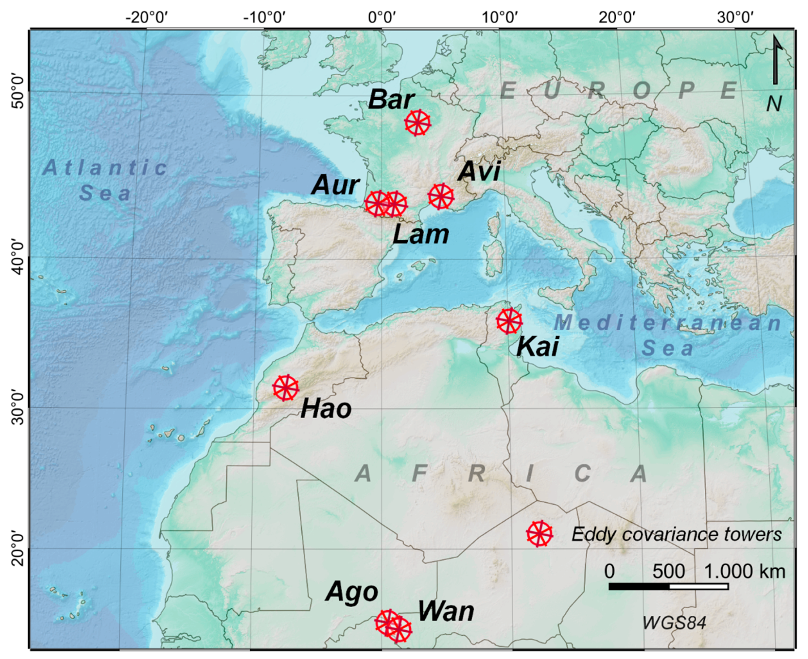
2.1. Experimental Datasets Description

The spatial distribution of the EC towers included in this work is found in Figure 1, whereas the main geographical details of each EC tower are summarized in

Table 1. Main geographical characteristics and data length of the EC towers included in this work.

Eddy Covariance Tower	Code	Country	Latitude/ Longitude	Elevation (m)	Years Analyzed	Köppen Climate Type	Ecosystem
Agofou	Ago	Níger	14°1′ N/1°25′ E	228	2009	BWh (Hot desert climate type)	Millet
Auradé	Aur	France	43°54′ N/01°10′ E	165	From 2006 to 2013	Cfb (Marine West Coast)	Wheat, sunflower
Avignon	Avi	France	43°55′ N/4°52′ E	32	From 2005 to 2013	Csa (Mediterranean)	Peas, wheat, sorghum and sunflower
Barbeau	Bar	France	48°29′ N/02°47′ E	90	From 2014 to 2015	Cfb (Marine West Coast)	Oak forest
Haouz	Hao	Morocco	31°67′ N/7°59′ W	450	2004	BSk (Mid-Latitude steppe climate)	Wheat
Kairouan	Kai	Tunisia	35°40′ N/10°05′ E	68	From 2012 to 2015	Csa (Mediterranean)	Olive and wheat
Lamasquère	Lam	France	43°49′ N/01°23′ E	185	From 2007 to 2013	Cfb (Marine West Coast)	Wheat
Wankama	War	Níger	13°6′ N/2°6′ E	207	2009	BWh (Hot desert climate type)	Savannah and millet

. The dataset analyzed includes daily records of vegetation greenness data (LAI), recorded with hemispherical photographs, once every 2 to 3 weeks, during specific stages of the phenological crop season. Haouz (Hao), Lamasquère (Lam) and Avignon (Avi) LAI records were validated with a planimeter using destructive methods. Days without LAI data were gap-filled with the broadly used local polynomial regression (LOESS) [31]. Meteorological, radiation budget and surface heat fluxes records were measured at meteorological EC towers. In this case, we used 30 min records of meteorological data (Ts, Rn, G and α) at 10:30 am and 1:30 pm, corresponding to typical sun-synchronous satellite overpass times. Meteorological records without data were excluded from the analysis. The data has been quality checked and previously used at [34]. Net radiation ratio records were acquired by a 4-component net radiometer (CNR1, 4.5–42 $\mu$m wavelength domain manufactured by Kipp & Zonen). Ground heat fluxes were acquired by self-calibrated heat plates sensors (HFP01SC, manufactured by HukseFlux) placed at different depths ranging from 5 cm to 100 cm. Depending on the site, different Ts measurement devices were installed. Further details of each site can be found below.

Barbeau (Bar) is located 60 km southeast of Paris (N of France) at 90 m of elevation. Bar is an oak-forest site (Fv > 0.95) under the Cfb climate influence, with a mean annual air temperature (MAAT) of 11 °C and a mean annual precipitation (MAP) of 680 mm. Ts was recorded by an infrared temperature sensor (IR120, 8–14 $\mathsf{\mu }$m wavelength domain manufactured by Campbell Scientific Inc.) (Logan, UT, USA) and a Type-T (manufactured by Thermocouple) sensor. An accurate description of the Bar site is provided at [35].

Moving southwards, at 25 km southwest of Toulouse (southwest France), two EC sites at a distance of 12 km are found: Auradé (Aur) and Lam. Aur (165 m of elevation) and Lam (185 m) sites are under the influence of a Cfb climate type, with a MAAT of 13 °C and MAP of 656 mm. Both of the EC sites include crops of wheat and sunflower (depending on the year), reaching mid to high LAI values (ca. 0.5; Figure 2a). Aur Ts was recorded by IRTS-P infrared sensors (6 to 14 $\mu$m wavelength domain, manufactured by Campbell Scientific Inc.) and a CS10X (manufactured by Campbell) sensor, placed at different depths from 4 to 100 cm under the surface. Lam Ts was calculated with upwelling longwave radiation data and an infrared temperature sensor CS-109 (manufactured by Campbell), with measurements at different depths ranging from 1 to 100 cm under the ground. Further technical details of Aur and Lam measurements can be found at [34,36].

Avignon (Avi) EC site is located northwest of Montpellier (southeast France), at 32 m of elevation. Avi is ruled by a Mediterranean climate type (Csa), with a MAAT of 14 °C and a MAP of 677 mm. Avi includes a wide range of crops types (depending on the season) such as peas, wheat and sorghum crops, and bare soil covers between crop seasons. Ts was calculated with upwelling longwave radiation data. A detailed technical description of the Avi can be found at [37].

Kairouan (Kai) is located in the Kairouan plain, in the South of Tunis (Tunisia) at 68 m of elevation. Kai is a crop site under the influence of a Csa climate type, with a MAAT of 20 °C and a MAP of 287 mm. Ts was measured with an infrared sensor (IR120; 8 to 14 µm wavelength, manufactured by Campbell Scientific Inc.), placed at 2.3 m height under the surface. Further details of Kai are found at [34], and references therein.

Haouz (Hao), is located in the Tunift basin, 45 km east of Marrakech (Morocco) at 450 m of elevation. Hao is under the influence of the BSk climate type, with a MAAT of 20 °C and a MAP of 150 mm, in an irrigated land of wheat crops. Ts was measured with a nadir-looking infrared radiometer (IRTS-P; 8 to 14 µm wavelength domain, manufactured by Campbell Scientific Inc.) at 2 m height. A detailed description of Hao is found at [38,39].

Furthermore, three EC towers were installed near Niamey (Niger) in a desert area under a BWh climate influence, with a MAAT of ca. 30 °C and a MAP of ca. 300 mm. Agofou (Ago) site is located in a millet zone, whereas in Wankama (Wan) one EC is located on the savannah, and another one is placed in a zone of wheat crops. Ts was recorded with an incidence thermal infrared thermometer (KT15; 8 to 14 m wavelength domain, manufactured by Heitronics) at 2.9 m height. Further details of the Niger EC sites can be found at [40,41].

The dataset has been gathered through the joint effort done between the international laboratories composed by (i) the Service National d’Observation (SNO), managed by the Institut National des Sciences de l’Univers (INSU), together with (ii) the NAILA laboratory, managed by the Institut National Agronomique de Tunisie (INAT), Institut National de Recherches en Génie Rural, Eaux et Forêts (INRGREF) and Institut de Recherce pour le Developpement (IRD); and (iii) the Télédétection et Ressources en Eau en Méditerranée semi-Aride (TREMA) organization, managed by the Université Cadi Ayyad (UCA), IRD, Agence de Basssin Hydaulique du Tensift (ABHT), Office Régional de Mise en Valeur Agricole du Haouz (ORMVAH), Direction de la Météorologie Nationale of Maroc (DMN) and the Centre National d’Etudes sur les Sciences les Techniques et l’Energie Nucléaire of Maroc (CNESTEN).

2.2. Methods

2.2.1. Estimation of Vegetation Indexes

Reflectance and biophysical variables (NDVI and Fv) were not available for the whole dataset. In this case, satellite-borne RS data could be biased, since the spatial resolution values of the data are the averages values for a given area, which does not correspond with the field-scale measurements recorded at each EC site. Hence, LAI values recorded with hemispherical photographs were converted to NDVI values following the method introduced by Clevers [42], and successfully applied and validated for all crop types [43]:

$$\mathrm{LAI}=-\frac{1}{k}\ln \left(\frac{{\mathrm{NDVI}}_{\infty }- \mathrm{NDVI} }{{\mathrm{NDVI}}_{\infty }-{ \mathrm{NDVI}}_{\mathrm{soil}} }\right)$$

(1)

$$\mathrm{NDVI}=\left(\left(\exp \left(\frac{\mathrm{LAI}}{{\mathrm{NDVI}}_{\infty }-{ \mathrm{NDVI}}_{\mathrm{soil}} }\right)x 0.80\right)-0.94\right)-1$$

(2)

where k is the calibrated extinction, set to 1.13 [43]. ${\mathrm{NDVI}}_{\infty }$ is the NDVI value of the fully developed canopy, whereas ${\mathrm{NDVI}}_{\mathrm{soil}}$ is the NDVI of bare soils. According to previous works, the ${\mathrm{NDVI}}_{\infty }$ was set to 0.97 [43]. We tested different ${\mathrm{NDVI}}_{\mathrm{soil}}$ values, ranging from 0 to 0.2, but no significant G/Rn differences were found. Therefore the ${\mathrm{NDVI}}_{\mathrm{soil}}$ was set to 0.1 [30].

The Fv was calculated with the semi-empirical method introduced by Roujean [44], where Fv is performed with the following exponential function of LAI:

$$\mathrm{Fv}=1-\exp \left(-\mathrm{b} x \mathrm{F}\left(\mathrm{o}\right) \mathrm{x} \mathrm{I} x \mathrm{LAI}\right)$$

(3)

where $\mathrm{b}$, $\mathrm{F}\left(\mathrm{o}\right)$ and $\mathrm{I}$ are constants, corresponding to −0.945, 0.5 and 1, respectively.

2.2.2. Empirical Equations and Machine Learning Algorithms

The empirical equations included in this work are divided into Type I and Type II. Type I gathers the empirical equations that estimate G with only vegetation indexes. This includes E1, E2 and E3 (based on NDVI), E4 and E5 (Fv), and finally E6 (LAI). Type II includes E7, which estimates G with Ts and LAI, and E8 which estimates G with NDVI, Ts and α. A detailed description of the empirical equations can be found in

Table 2. Empirical equations and ML algorithms used for the estimation of the G.

Empirical Equations and ML Code	Empirical Equation	Calibrated Values	Further Details
E1	a − b x NDVI	a = 0.3, b = 0.26	[19]
E2	a x exp(−b x NDVI)	a = 0.39, b = 1.952	[10]
E3	a x (NDVI) + b	a = 0.47, b = 0.43	[10,45]
E4	a x (1 − Fv)	a = 0.23	[25]
E5	−a + (1 − Fv) x (b − c)	a = 0.015, b = 0.315, c = 0.064	[10]
E6	a x exp(−b x LAI)	a = 0.23, b = 0.45	[24]
E7	If LAI < 0.5 = $-\frac{\mathrm{a} \mathrm{x} \left(\mathrm{Ts} –273.15\right)}{\mathrm{Rn}+\mathrm{b}}$ If LAI > 0.5 = $\mathrm{c}+\mathrm{d} \mathrm{x} \exp \left(-\mathrm{e} \mathrm{x} \mathrm{LAI}\right)$	a = 1.7, b = 0.079, c = 0.05, d = 0.12, e = 0.621	[28]
E8	Ts x Rn x 0.0038 + 0.074 x α x (1 − 0.98 x NDVI^4)	$\mathrm{a}=0.06$, $\mathrm{b}=0.012$, c = 0.978	[20]
NN	Size From 10 to 30, increments of 5	20	[46]
	Decay From 0.001 to 0.2, increments of 0.05	0.15
RF	Ntree 50,100,200,400 and 800	800	[47]
	Mtry From 1 to 15, increments of 1	1

. Regarding the ML algorithms, NN I and RF I (ML I) are trained with LAI data, providing a fair comparison with Type I equations. Neural network II and RF II (ML II) are trained with LAI and Ts. Last, NN III and RF III (ML III) are trained with LAI, Ts and Rn.

Neural Networks (NN)

The NN algorithm creates a distributed system of neurons with non-linear functions and several layers interconnected for the prediction of one variable, in this case, G. In this work we tuned the two principal hyper-values of the NN, named size and decay (Table 2). The parametrization of the NN size ranged from 10 to 30, with increments of 5; while the parametrization of the decay ranged between 0.001 and 0.2, with increments of 0.05. An accurate description of the mathematical formulation of the NN can be found at [46,48].

Random Forest (RF)

The RF method is a non-parametric method based on decision trees and bootstrap aggregation [47]. A group of trees is developed using multiple decision trees trained from random subsets of the dataset. In this work, we applied the regression version of the RF, where the estimated values are the result of the arithmetic average of all the tree predictions (M). The trees {${\mathrm{M}}_1\left(\mathrm{X}\right),{\mathrm{M}}_1\left(\mathrm{X}\right),\dots , {\mathrm{M}}_{\mathrm{K}}\left(\mathrm{X}\right)$}, where X = {x1, x2, …, xβ}, being β-dimension input vector that creates a forest. The ensembles generate P values that correspond to the tree ${\mathrm{Y}}_{\mathrm{p}}$ (p = 1, 2, …, P).

The RF regression is calculated as follows:

$$f\left(x\right)=\frac{1}{\mathrm{M}}{{\displaystyle \sum }}_{\mathrm{m}=1}^{\mathrm{M}} {\mathrm{M}}_k\left(x_j\right)$$

(4)

The tunning of the regression RF has been analyzed at [49]. In their study, they conclude that the number of decision trees randomly selected in the model, the subset of training samples, together with the variables split at each tree node, prevents the algorithm from overfitting. Two hyper-values have been tuned of the RF. The number of predictors evaluated in each node (mtry), and the number of trees (ntree) of a random sample. We performed a sensitivity analysis of the RF hyper-values (Table 2), but no significant differences were found in the accuracy metrics (Table S1). In this work, the mtry was set as 1 and the ntree was equal to 800.

We used a grid search and 10-fold cross-validation to validate the hyper-values of both of the ML algorithms. We applied the RF with the randomForest package [50] and the NN with the Caret package [51], both of them of R Studio [52].

2.3. Evaluation

In order to avoid the evaluation of the methods over the same training data, the initial dataset was randomly split into two groups. The training dataset (conforming the 70% of the dataset) and the testing dataset (which constitutes the remaining 30%). In the training dataset, the empirical equations have been calibrated and the ML algorithms tuned. Table 2 shows the different ML hyper-values tested and the values set, as well as the calibrated constant values of the empirical equations. Subsequently, the trained ML algorithms and the calibrated empirical equations have been applied in the independent and testing dataset. Hence, the results obtained with the calibrated empirical equations and the trained ML algorithms are comparable, given that the evaluation and calibration of all the methods have been performed under the same conditions. We also evaluated the accuracy and performance of each method by Fv ranges, from 0 to 1, in increments of 0.25. The accuracy and performance of the models have been evaluated using four types of statistical metrics: the residual (Equation (5)), the mean absolute error (MAE; Equation (6)), the Root Mean Square Error (RMSE; Equation (7)), the coefficient of determination (R²; Equation (8)) and Willmott’s D (D; Equation (9)).

$$\mathrm{Residual}=yi-\widehat{y}$$

(5)

$$\mathrm{MAE}=\frac{1}{N}{\displaystyle \sum }_{i=1}^N\left|yi-\widehat{y}\right|$$

(6)

$$\mathrm{RMSE}=\sqrt{\frac{1}{N}{\displaystyle \sum }_{i=1}^N{\left(yi-\widehat{y}\right)}^2}$$

(7)

$${\mathrm{R}}^2=1- \frac{{\displaystyle \sum }{\left(yi-\widehat{y}\right)}^2}{{\displaystyle \sum }{\left(yi-\overline{y}\right)}^2}$$

(8)

$$\mathrm{Willmott}’\mathrm{s} \mathrm{D}=1-\sqrt{\frac{{{\displaystyle \sum }}_{\mathrm{i}=1}^{\mathrm{N}}{\left(yi-\widehat{y}\right)}^2}{{{\displaystyle \sum }}_{\mathrm{i}=1}^{\mathrm{N}}{\left(\left|yi\right|-\left|\widehat{y}\right|\right)}^2}}$$

(9)

where N is the number of the samples $yi$ is the observed value, $\widehat{y}$ is the estimated and $\overline{y}$ represents the average value of the estimated values. The residual is the difference between $yi$ and $\widehat{y}$. The MAE and RMSE summarise the mean differences between the predicted values and the observed values. Low RMSE and MAE values are inversely related to the high accuracy of the method proposed. The RMSE is sensitive to high values or outliers [53] and can be used as an indicator of the magnitude of extreme errors. On the contrary, high values of D and R² are related to the high performance of the methods.

3. Results and Discussion

In the first section we determine which are the meteorological and vegetation drivers of G. Subsequently, we analyze the observed and estimated values of the heat flux. Then, we provide a detailed analysis of the accuracy and performance metrics of all the methods, together with an evaluation of the methods by Fv ranges. The results are discussed and compared with previous works. Finally, we elaborate on the reason for the good accuracy and performance metrics obtained with ML.

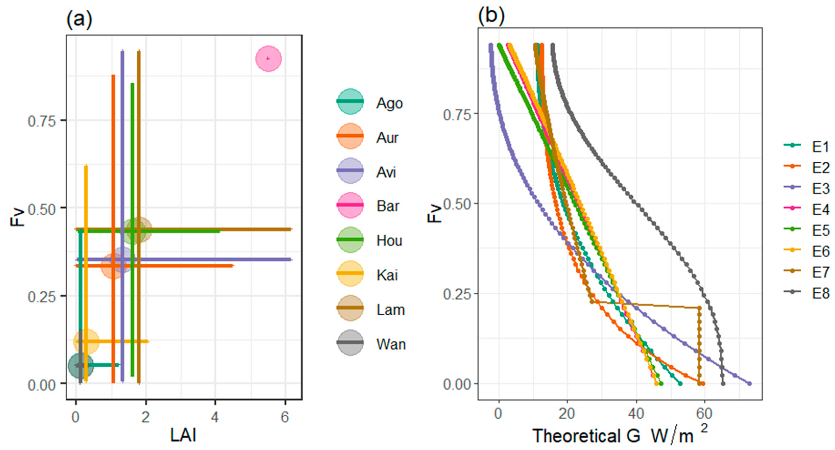
3.1. Characterization and Drivers of G

The G values expected by each equation with the same sample data are shown in the theoretical plot presented in Figure 2b. Both of the empirical equation’s types, based only on vegetation indexes (Type I); as well as on vegetation indexes, ancillary remote sensing and meteorological data (Type II) estimate an overall decrease of the G depending on Fv. In bare soils and sparse vegetation areas (Fv ≤ 0.25), the equations suggest that G supposes ≥ 20 W/m² of the SEB, providing evidence that G is not a negligible SEB component, in these land cover conditions [31]. For mid to high vegetation ranges (Fv > 0.25), the E1, E2, E4, E5, E6 and E7 show a parallel shape for the G estimation, and hence similar values can be expected. The highest difference between equations is found between E3 and E8. Whilst the equations have a curve shape for Fv > 0.4, for bare soils and sparse vegetation areas E8 assumes a constant G value, and E3 estimates G as an exponential function of Fv (Figure 2b).

Figure 2. (a) Maximum, minimum and mean Fv (y-axis) and LAI (x-axis) values of the EC included in this work. (b) Theoretical shape of the empirical equations based on vegetation indexes. Values of G were estimated with sample values of the input biophysical variables and constant values of the meteorological data. Equations E7 and E8 do not only rely on vegetation data. We assumed the meteorological input parameters of E7 and E8 as constant. Ts was = 25 °C, α = 0.4 and Rn = 200 W/m².

Figure 2. (a) Maximum, minimum and mean Fv (y-axis) and LAI (x-axis) values of the EC included in this work. (b) Theoretical shape of the empirical equations based on vegetation indexes. Values of G were estimated with sample values of the input biophysical variables and constant values of the meteorological data. Equations E7 and E8 do not only rely on vegetation data. We assumed the meteorological input parameters of E7 and E8 as constant. Ts was = 25 °C, α = 0.4 and Rn = 200 W/m².

Figure 3 shows evidence that the different drivers of G depend on the Fv range. For bare soils and sparse vegetation areas, the best parameter for estimating G is Ts (R² = 0.48), followed by Rn (R² = 0.30). Over densely vegetated areas and high canopies (Fv ≥ 0.50), the minimum G values are observed (ca. 5 W/m²). On many days, the G can be neglected or be assumed to be practically equal to 0 [19]. This is because high levels of vegetation cover thermally insulate the surface, significantly reducing the solar radiation that reaches the ground [54], and buffering temperature gradients in areas with significant rates of ET [31]. Given that the G variability under densely vegetated areas and high canopies is not mainly ruled by Rn and Ts, the incorporation of these variables as a predictor variable is redundant.

The observed and estimated G values by the different empirical equations and ML algorithms are shown in Figure 3 and Figure 4. The observed mean value of G ranged from 59 to 18 W/m². In bare soils and sparse vegetation areas, where the majority of the data is found (Figure 2a), the highest G values are measured in accordance with previous works [21]. In these land types, characteristics of arid and semiarid climates zones, the highest values of G are generally observed during the warmest months of the year [31]. The G rules a significant part of the SEB hourly variability, with instantaneous G values ranging from 5–10% up to 50% of the Rn [30,55,56].

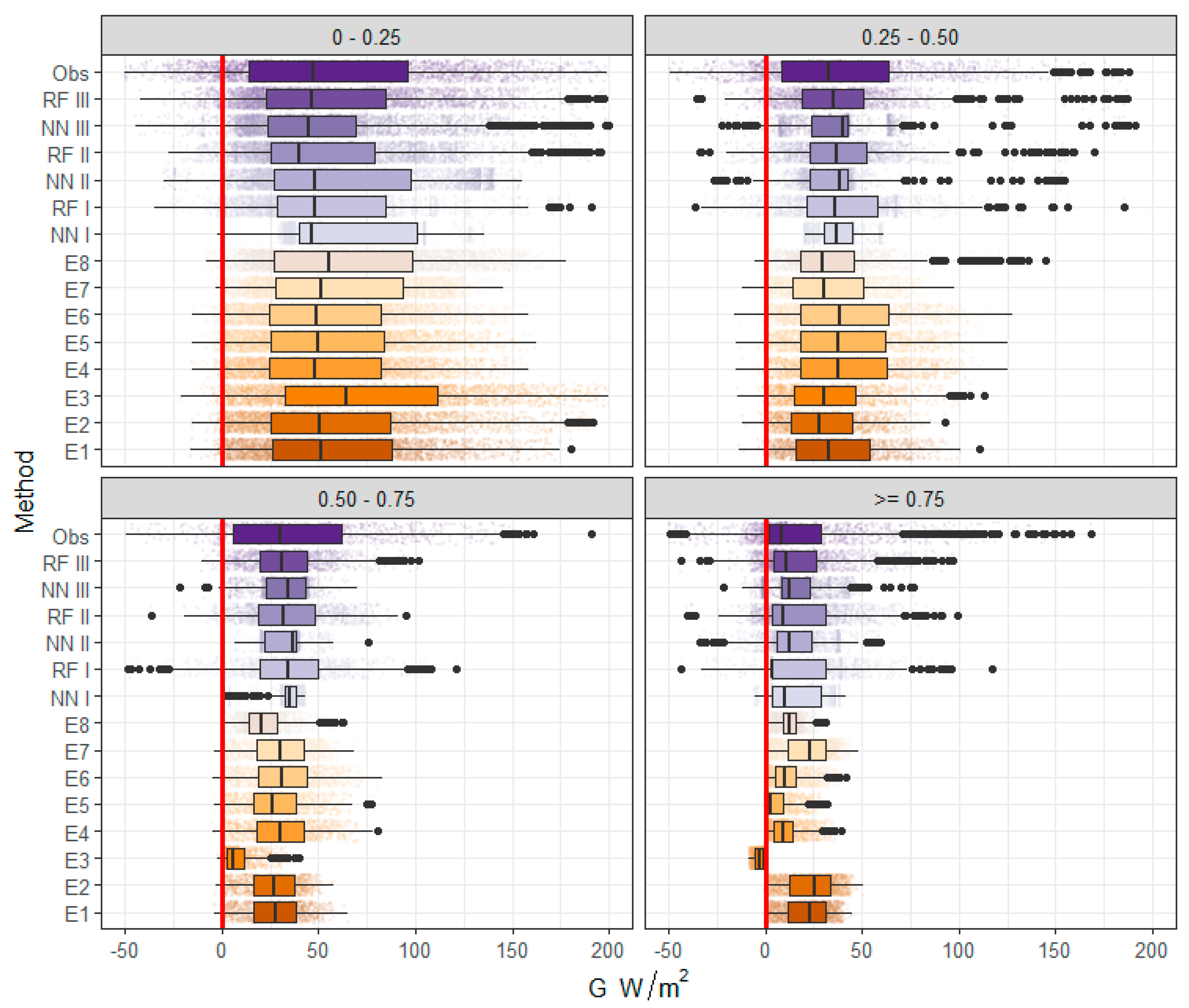
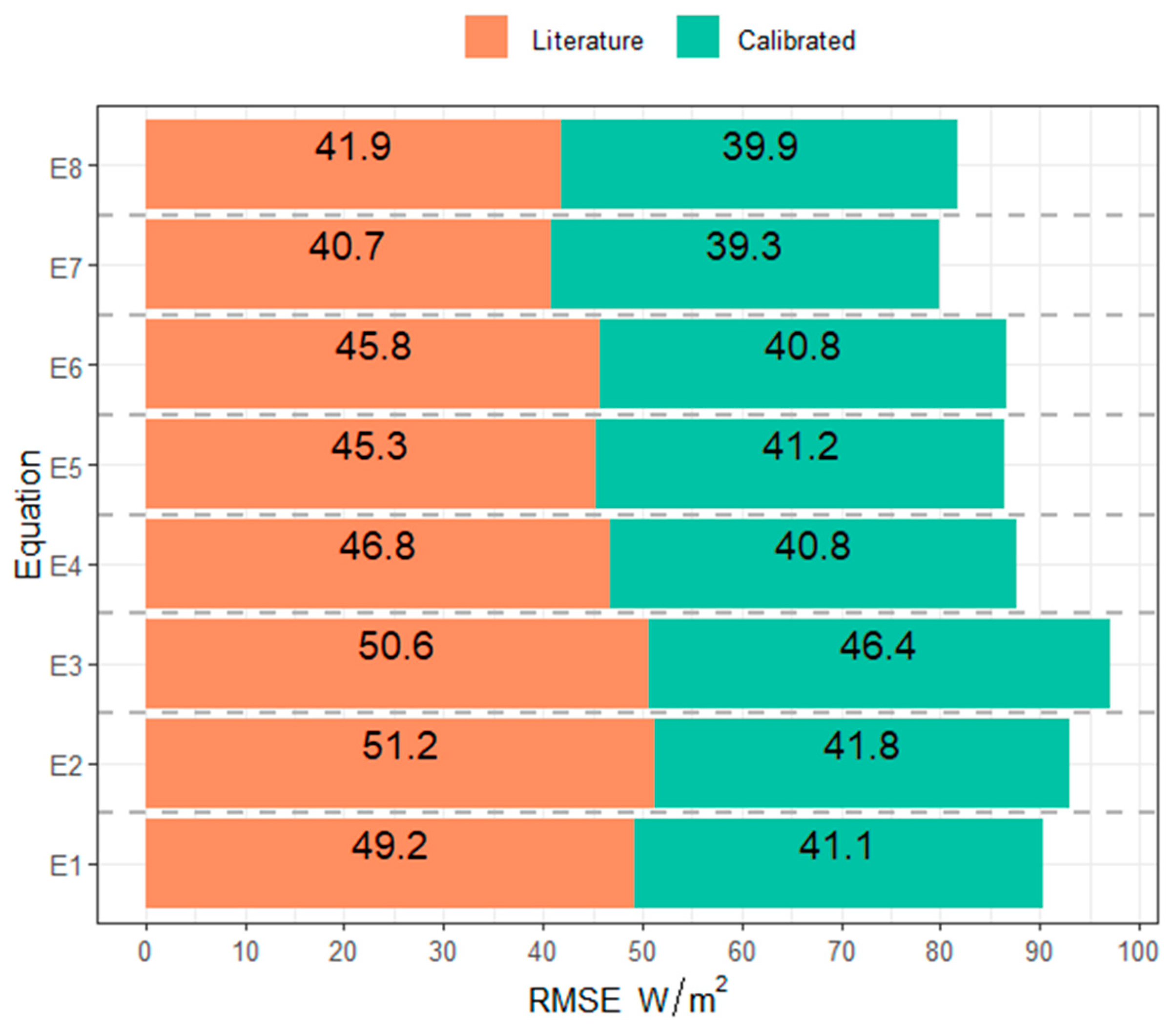
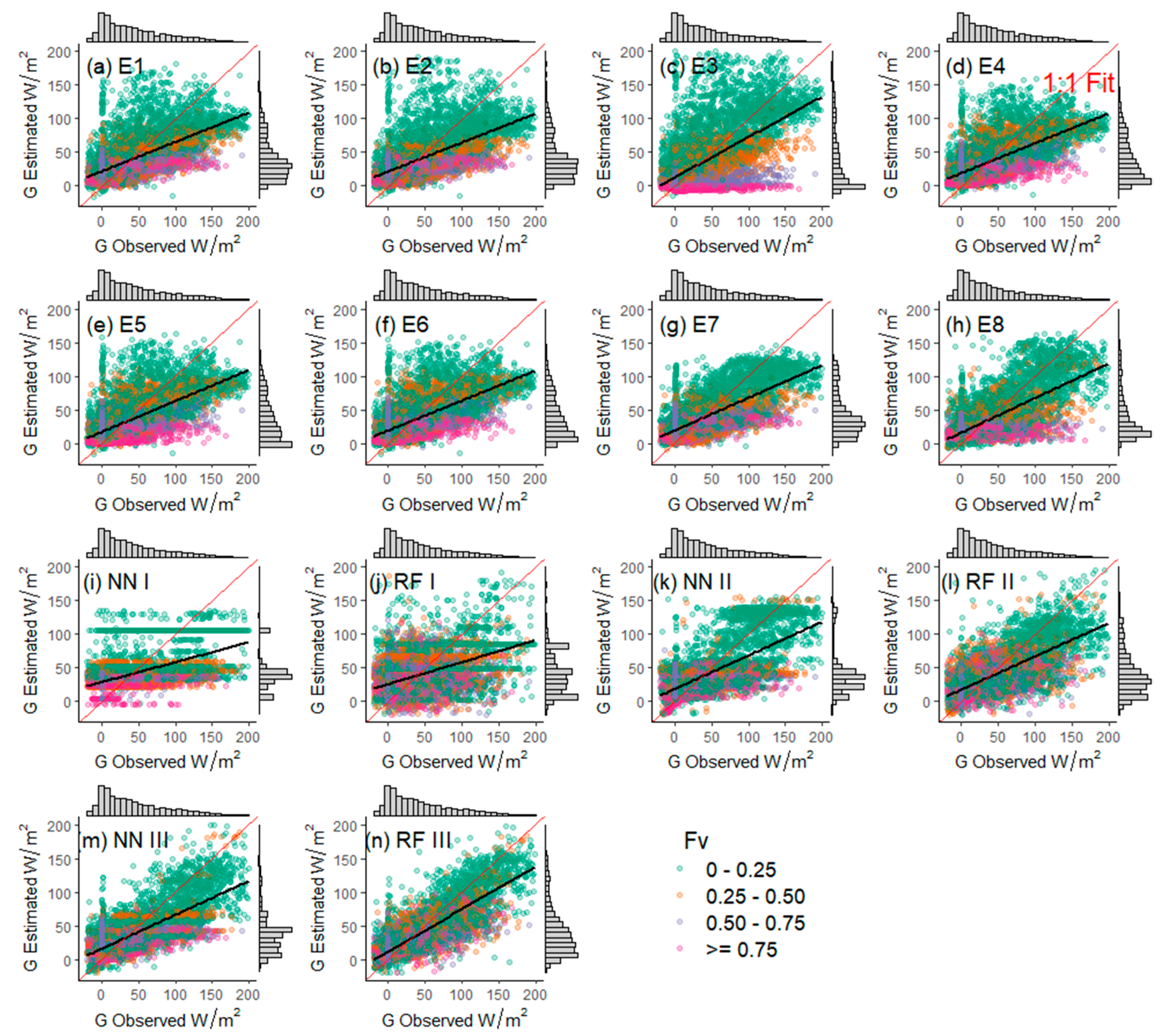
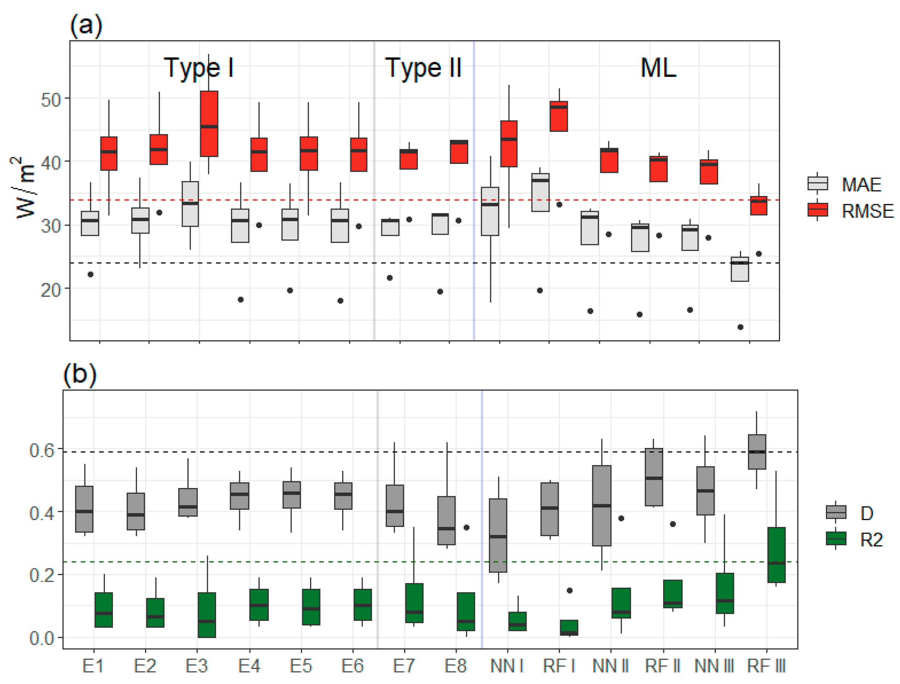
3.2. Analysis of the Accuracy and Performance of the Different Methods Used for the Estimation of G

The calibration of the constant values slightly improved the Type I equation’s accuracy, but negligible differences are found for Type II equations (Figure 5). Regarding the ML models, no significant differences in the accuracy metrics have been observed between the training and the testing dataset, providing evidence of the lack of overfitting. In addition, negligible differences have been found between the different hyper-values tested during the ML tunning process (Table S1).

The majority of the empirical equations have shown a systematic underestimation of G, specially E3 for Fv ≥ 0.75. The highest bias is observed with the empirical equations that conform to Type I. The residual term (the difference between the estimated and the observed values) of Type I increases with Fv, except for E4 and E6. On the other hand, Type II overestimates G for bare soils and sparse vegetation areas (5 W/m²) and underestimates the heat flux for the other Fv ranges. The residual term for Type I is larger in densely vegetated areas and high canopies covers (>5 W/m²) than in bare soils and sparsely vegetated areas, and therefore the data suggest that Type I equations are not able to reproduce the decrease of G depending on Fv. This is because Type I equations determine a constant value for all the Fv ranges. In contrast, other empirical equations such as E7, use a threshold as a function of LAI, determining two empirical equations for the estimation of G (Table 2) and in the end providing better results.

The estimation of G with ML has shown lower residual differences than those obtained with the empirical equations (Figure 6). In fact, the residual term with ML is practically the same (avg. ca. 5 W/m²) for the majority of Fv ranges. In addition, no systematic biases are estimated with ML II and ML III. Furthermore, ML II and III are able to reproduce the highest (percentile 90th) G values (Figure 3). The validation metrics by Fv ranges are shown in

Table 3. Accuracy and performance metrics of each method, grouped by Fv ranges.

Metric	FV	E1	E2	E3	E4	E5	E6	E7	E8	NN I	RF I	NN II	RF II	NN III	RF III
MAE	0–0.25	36.6	37.3	39.8	36.6	36.5	36.6	31	31.6	40.7	39	30.4	29.9	29	23.6
	0.25–0.50	30.4	31.2	31.1	30.4	30.3	30.4	30.7	31.8	34.3	37.8	31.9	30.7	29.6	24.5
	0.50–0.75	30.7	30.7	35.9	31	31.2	31	30.7	31.6	31.9	36.2	32.4	29.1	30.9	25.9
	≥0.75	22.2	23	26	18.1	19.6	18	21.6	19.5	17.8	19.7	16.4	15.8	16.6	13.9
RMSE	0–0.25	49.7	50.9	56.9	49.2	49.3	49.2	43	43.4	52.0	51.4	41.6	41.3	39.8	33.9
	0.25–0.50	41	42	41.9	41.2	41.1	41.3	41.4	42.6	44.5	48.7	41.8	40.7	39.2	33.6
	0.50–0.75	41.8	41.9	49.3	41.9	42.2	41.9	41.6	43.4	42.5	48.4	43.1	39.7	41.7	36.4
	≥0.75	31.3	32	37.9	30	31.5	29.7	30.9	30.6	29.5	33.2	28.5	28.3	28	25.4
D	0–0.25	0.6	0.5	0.6	0.5	0.5	0.5	0.6	0.6	0.4	0.5	0.6	0.6	0.6	0.7
	0.25–0.50	0.5	0.4	0.4	0.5	0.5	0.5	0.4	0.4	0.2	0.3	0.3	0.4	0.4	0.6
	0.50–0.75	0.3	0.3	0.4	0.3	0.3	0.3	0.3	0.3	0.2	0.3	0.2	0.4	0.3	0.5
	≥0.75	0.3	0.3	0.4	0.4	0.4	0.4	0.4	0.3	0.5	0.5	0.5	0.6	0.5	0.6
R2	0–0.25	0.2	0.2	0.3	0.2	0.2	0.2	0.3	0.3	0.1	0.1	0.4	0.4	0.4	0.5
	0.25–0.50	0.1	0.1	0.1	0.1	0.1	0.1	0.1	0.1	0	0	0	0.1	0.1	0.3
	0.50–0.75	0	0	0	0	0	0	0	0	0	0	0	0.1	0	0.2
	≥0.75	0	0	0	0.1	0	0.1	0	0	0.1	0	0.1	0.1	0.1	0.2

and Figure 7 and Figure 8. The results provide evidence that the estimation of G based on Type I empirical equations leads to high uncertainties in comparison with the ML methods. The error metrics for the majority of the Type I empirical equations are practically the same under bare soils and scarce vegetated areas (MAE = 36 and RMSE = 51 W/m²). Nevertheless, the highest differences between Type I equations are observed in densely vegetated areas. The accuracies of E1, E2 and E3 are worse than the group constituted by E4, E5 and E6 (avg. MAE 24 vs. 18 W/m²), confirming the E1, E2 and E3 systematic underestimation of the G. Type II improve the estimation of G to some degree. The accuracy of E8 (MAE = 28, RMSE = 39 W/m²) is slightly better than the E7 (MAE = 28, RMSE = 37 W/m²), but two Type I equations (E4 and E6) outperformed all the empirical equations for the estimation of G at dense and high canopies covers. Therefore, these results suggest that the estimation of G is more accurate with Fv data (E4 and E5) and LAI (E6) than with NDVI (E1, E2 and E3). The results presented in this article are in accordance with previous studies that estimated the G based on vegetation indexes [10,19,31]. The lack of difference between E7 and E8 suggests that the inclusion of α in the empirical formulations that already include Ts does not substantially improve the estimation of G. This is probably explained because of the collinearity existent between Ts and α.

ML I, which only includes LAI as a predictor variable, shows similar accuracy metrics as Type I and hence a low performance for the estimation of G. Machine learning II, which includes LAI and Ts as predictor variables, outperformed all the empirical equations. Moreover, ML III, including LAI, Ts and Rn, significantly improved all the estimations of G and showed the best accuracy and performance (Figure 6, Figure 7 and Figure 8). In particular, RF II shows slightly better results than NN II. Yet, the difference between algorithms increases when Rn is included in the regression models (Table 3). Except for E4, in bare soils and sparse vegetation areas, Type I error is almost double (MAE = 39.8 W/m²) than that measured with the RF III (MAE = 23.6 W/m²). Furthermore, the performances of RF III by Fv ranges are more constant than the other methods. The minimum errors are observed in bare soils and sparse vegetation areas (D = 0.7 and R² = 0.5), which could be explained because the majority of the data is found in this Fv range. In densely vegetated areas, the RF III performed also better than all the other methods. For instance, at Fv > 0.5, the R² values of RF III are 0.3, whereas the other methods rarely reach an R² of 0.1 (Figure 8). However, NN III and RF III do not significantly improve the large uncertainty in the highest vegetation range (Fv ≥ 0.75). For NN III, the D and R² values are only 0.3 and 0.1, respectively. Random forest III shows a slightly better performance, with a D and an R² of 0.3 and 0.2, respectively.

Uncertainties in the SEB fluxes quantification can be related to measurement bias, which corresponds with ca. 10% for G, and ca. 5% for Rn [21]. However, all the methods have been evaluated under the same conditions, and hence the superiority of RF II and III is related to the algorithm architecture. The regression-based ML methods have shown promising results over the last years for the prediction of continuous variables, and have been successfully applied in a wide range of scientific disciplines, including climate and hydrological modelling [57]. For example, ML provides better results than Multiple Linear Regression for the spatial interpolation of air temperature [58]. Machine learning also has shown optimal results for the estimation of environmental variables, such as H and LE retrievals [59], other SEB components such as Rn and H [60,61] or ET [62,63,64]. For the estimation of G, Canelón et al. [32] modelled the heat flux with ANN and RS data, and de Andrade et al. [33] compared the ANN and two empirical equations based on NDVI, Ts and $\mathsf{\alpha }$. In accordance with our findings, in both of the works, ML outperformed the other methods for the estimation of G. The underestimation of the empirical equations and the large errors found at high Fv ranges are partly because the majority of Type I and II equations rely on a single linear relationship with the predictor variables. The main strengths of the NN and RF are that they are very flexible, adaptable to the shifting G values depending on the vegetation and meteorological conditions, and do not follow a stationary and linear assumption. The bootstrap aggregating (bagging) algorithms, such as RF, creates several models by selecting a random subset of the variable for each decision tree. Moreover, the inclusion of Rn in RF III improved the G estimation, showing evidence that the recursive model partitioning of RF is resistant to overlaps in the covariates, and can handle correlated variables such as Rn and Ts. In addition, RF is a non-parametric model, to overcome noise and outliers [49]. On the other hand, the limitation of the ML algorithms is that generally reproduce the data of the training dataset, and could not extrapolate the values outside of the training. The estimation of G with ML also requires more computational time than the empirical equations. The training time required to train the RF algorithms was equal to 5, 8 and 11h for RF I, II and III, respectively. On the contrary, the training time of the NN was 26, 28 and 31′ for NN I, II and III, respectively. Nonetheless, once the ML algorithms are trained, they are computationally efficient. In this case, the prediction time required was lower than one minute. Finally, further research is needed in order to improve the energy balance closure and the estimation of G in high canopies covers. If the accuracy between ML methods shows small differences, the introduction of other predictor variables should be tested. Further works should focus to combine ML with physical modelling [62].

4. Conclusions

Anthropogenic climate change is leading to changes in the water and energy fluxes of some areas of the planet, such as the tropical and mid-latitude regions. Therefore, accurate hydrological estimation is crucial in order to better quantify water balances, and support socioecological decision-making. This work compared different methods for the estimation of a SEB component with large uncertainties, the G. For the first time, we evaluated an ensemble ML method (the RF), against NN and several empirical equations that have been extendedly used for decades for the estimation of G with RS data. The evaluation was performed using data from EC sites, with a wide range of vegetation (i.e., forests, crops of wheat or millet) and climate (from the marine west coast to desert) types, along the mid-latitude area found between continental Europe up to the middle of the African continent.

The data have shown that the driver of G depends on the Fv range. In bare soils and sparse vegetation areas, Rn followed by Ts rules the estimation of G, decreasing with Fv. On the contrary, meteorological and vegetation data have not shown a relevant and statistically significant link with the estimation of G in densely vegetated areas. Neural network and RF models, with LAI and Ts as predictor variables, outperform the empirical equations for the estimation of the G, independent of the Fv range considered. The inclusion of Rn in the model significantly improved the estimation of G. Despite the computational time required (8 h), RF III have shown the highest R², D as well as the lowest MAE and RMSE. The accuracy values of the empirical equations are almost double when compared to the measured values with RF III. Further works should analyze the estimation of G over large areas with the predictor variables used here, in combination with other predictor variables, for instance, downscaled soil moisture data. Also, further research could test the combination of ML with physical-based models for the estimation of G.

References

1. Giorgi, F. Climate change hot-spots. Geophys. Res. Lett. 2006, 33, L08707. [Google Scholar] [CrossRef]
2. Hu, Y.; Fu, Q. Observed poleward expansion of the Hadley circulation since 1979. Atmos. Chem. Phys. 2007, 7, 5229–5236. [Google Scholar] [CrossRef] [Green Version]
3. De Luis, M.; Brunetti, M.; Gonzalez-Hidalgo, J.C.; Longares, L.A.; Martin-Vide, J. Changes in seasonal precipitation in the Iberian Peninsula during 1946–2005. Glob. Planet Chang. 2010, 74, 27–33. [Google Scholar] [CrossRef]
4. Vicente-Serrano, S.M.; Lopez-Moreno, J.I.; Beguería, S.; Lorenzo-Lacruz, J.; Sanchez-Lorenzo, A.; García-Ruiz, J.M.; Azorin-Molina, C.; Morán-Tejeda, E.; Revuelto, J.; Trigo, R.; et al. Evidence of increasing drought severity caused by temperature rise in southern Europe. Environ. Res. Lett. 2014, 9, 044001. [Google Scholar] [CrossRef]
5. Orlowsky, B.; Seneviratne, S.I. Global changes in extreme events: Regional and seasonal dimension. Clim. Chang. 2012, 110, 669–696. [Google Scholar] [CrossRef] [Green Version]
6. Giorgi, F.; Lionello, P. Climate change projections for the Mediterranean region, Global Planet. Change 2008, 63, 90–104. [Google Scholar] [CrossRef]
7. Sheffield, J.; Wood, E.F. Projected changes in drought occurrence under future global warming from multi-model, multi-scenario, IPCC AR4 simulations. Clim. Dynam. 2008, 31, 79–105. [Google Scholar] [CrossRef]
8. Viviroli, D.; Durr, H.; Messerli, B.; Meybeck, M.; Weingartner, R. Mountains of the world, water towers for humanity: Typology, mapping, and global significance. Water Resour. Res. 2007, 43, W07447. [Google Scholar] [CrossRef] [Green Version]
9. Boulet, G.; Jarlan, L.; Olioso, A.; Nieto, H. Evapotranspiration in the Mediterranean region. In Water; Brocca, L., Tramblay, Y., Molle, F., Eds.; Elsevier: Amsterdam, The Netherlands, 2020; pp. 23–49. [Google Scholar]
10. Kpemlie, E. Assimilation Variation Nelle De Donnees De Télédétection Dans Des Modèles De Fonctionnements Des Couverts Végétaux et Du Paysage Agricole. Ph.D. Thesis, Université d’Avignon et des Pays de Vaucluse, Avignon, France, 2009. [Google Scholar]
11. Sauer, T.J.; Horton, R. Soil heat flux. In Micrometeorology in Agricultural Systems; Hatfield, J.L., Baker, J.M., Eds.; American Society of Agronomy: Madison, WI, USA, 2005; pp. 131–154. [Google Scholar] [CrossRef]
12. Liebethal, C.; Foken, T. Evaluation of six parameterization approaches for the ground heat flux. Theor. Appl. Climatol. 2007, 88, 43–56. [Google Scholar] [CrossRef]
13. Shao, C.; Chen, J.; Li, L.; Xu, W.; Chen, S.; Gwen, T. Spatial variability in soil heat flux at three Inner Mongolia steppe ecosystems. Agric. For. Meteorol. 2008, 148, 1433–1443. [Google Scholar] [CrossRef]
14. Venegas, P.; Grandón, A.; Jara, J.; Paredes, J. Hourly estimation of soil heat flux density at the soil surface with three models and two field methods. Theor. Appl. Climatol. 2013, 112, 45–59. [Google Scholar] [CrossRef]
15. An, K.; Wang, W.; Wang, Z.; Zhao, Y.; Yang, Z.; Chen, L.; Zhang, Z.; Duan, L. Estimation of ground heat flux from soil temperature over a bare soil. Theor. Appl. Climatol. 2017, 129, 913–922. [Google Scholar] [CrossRef]
16. Gao, Z.; Russell, E.S.; Missik, J.E.C.; Huang, M.; Chen, X.; Strickland, C.E.; Clayton, R.; Arntzen, E.; Ma, Y.; Liu, H. A novel approach to evaluate soil heat flux calculation: An analytical review of nine methods. J. Geophys. Res. Atmosph. 2017, 122, 6934–6949. [Google Scholar] [CrossRef]
17. Murray, T.; Verhoef, A. Moving towards a more mechanistic approach in the determination of soil heat flux from remote measurements. I. A universal approach to calculate thermal inertia. Agric. For. Meteorol. 2007, 147, 80–87. [Google Scholar] [CrossRef]
18. Murray, T.; Verhoef, A. Moving towards a more mechanistic approach in the determination of soil heat flux from remote measurements. II. Diurnal shape of soil heat flux. Agric. For. Meteorol. 2007, 147, 88–97. [Google Scholar] [CrossRef]
19. Kustas, W.P.; Daughtry, C.S.T. Estimation of the soil heat flux/net radiation ratio from spectral data. Agric. For. Meteorol. 1990, 49, 205–233. [Google Scholar] [CrossRef]
20. Bastiaanssen, W.G.M.; Menenti, M.; Feddes, R.A.; Holslag, A.A.M. A remote sensing surface energy balance algorithm for land (SEBAL): 2 Validation. J. Hydrol. 1998, 212–213, 213–219. [Google Scholar] [CrossRef]
21. Santanello, J.A.; Friedl, M.A. Diurnal variation in soil heat flux and net radiation. J. Appl. Meteor. 2003, 42, 851–862. [Google Scholar] [CrossRef]
22. Cellier, P.; Richard, G.; Robin, P. Partition of sensible heat fluxes into bare soil and the atmosphere. Agric. For. Meteorol. 1996, 82, 245–265. [Google Scholar] [CrossRef]
23. Kustas, W.P.; Daughtry, C.S.T.; Van Oevelen, P.J. Analytical treatment of the relationship between soil heat flux/net radiation ratio and vegetation indices. Remote Sens. Environ. 1993, 46, 319–330. [Google Scholar] [CrossRef]
24. Choudhury, B.J.; Idso, S.B.; Reginato, R.J. Analysis of an empirical model for soil heat flux under a growing wheat crop for estimating evapotranspiration by an infrared-temperature based energy balance empirical equation. Agric. For. Meteorol. 1987, 39, 283–297. [Google Scholar] [CrossRef]
25. Anderson, M.C.; Norman, J.M.; Mecikalski, J.R.; Otkin, J.A.; Kustas, W.P. A climatological study of evapotranspiration and moisture stress across the continental U.S. based on the thermal remote sensing: I. Model formulation. J. Geophys. Res. Lett. 2007, 112, D10117. [Google Scholar] [CrossRef]
26. Sobrino, J.A.; Gómez, M.; Jiménez-Muñoz, J.C.; Olioso, A.; Chehbouni, G.A. simple algorithm to estimate evapotranspiration from DAIS data: Application to the DAISEX Campaigns. J. Hydrol. 2005, 315, 117–125. [Google Scholar] [CrossRef] [Green Version]
27. Miralles, D.G.; Holmes, T.R.H.; De Jeu, R.A.M.; Gash, J.H.; Meesters, A.G.C.A.; Dolman, A.J. Global land-surface evapotranspiration estimated from satellite-based observations. Hydrol. Earth Sys. Sci. 2011, 15, 453–469. [Google Scholar] [CrossRef] [Green Version]
28. Allen, R.G.; Tasumi, M.; Trezza, R. Satellite-based energy balance for mapping evapotranspiration with internalized calibration (METRIC). Model. J. Irrig. Drain. Eng. 2007, 133, 380–394. [Google Scholar] [CrossRef]
29. Bastiaanssen, W.G.M. SEBAL-based sensible and latent heat fluxes in the irrigated Gediz Basin, Turkey. J. Hydrol. 2000, 229, 87–100. [Google Scholar] [CrossRef]
30. Sun, Z.; Gebremichael, M.; Wang, Q. Evaluation of empirical remote sensing-based empirical equations for estimating soil heat flux. J. Meteorol. Soc. Jpn. 2013, 91, 627–638. [Google Scholar] [CrossRef] [Green Version]
31. Purdy, A.; Fisher, J.; Goulden, M.; Famiglietti, J. Ground heat flux: An analytical review of 6 models evaluated at 88 sites and globally. J. Geophys. Res. Biog. 2016, 121, 3045–3059. [Google Scholar] [CrossRef]
32. Canelón, D.J.; Chávez, J.L. Soil heat flux modeling using artificial neural networks and multispectral airborne remote sensing imagery. Remote Sens. 2011, 3, 1627–1643. [Google Scholar] [CrossRef] [Green Version]
33. De Andrade, B.C.C.; Pedrollo, O.C.; Ruhoff, A.; Moreira, A.A.; Laipelt, L.; Kayser, R.B.; Biudes, M.S.; dos Santos, C.A.C.; Roberti, D.R.; Machado, N.G.; et al. Artificial neural network model of soil heat flux over multiple land covers in South America. Remote Sens. 2021, 13, 2337. [Google Scholar] [CrossRef]
34. Delogu, E.; Boulet, G.; Olioso, A.; Garrigues, S.; Brut, A.; Tallec, T.; Demarty, J.; Soudani, K.; Lagouarde, J.-P. Evaluation of the SPARSE Dual-Source Model for Predicting Water Stress and Evapotranspiration from Thermal Infrared Data over Multiple Crops and Climates. Remote Sens. 2018, 10, 1806. [Google Scholar] [CrossRef] [Green Version]
35. Chemidlin Prévost-Bouré, N.; Soudani, K.; Damesin, C.; Berveiller, D.; Lata, J.-C.; Dufrêne, E. Increase in above ground fresh litter quantity over-stimulates soil respiration in a temperate deciduous forest. Appl. Soil Ecol. 2010, 46, 26–34. [Google Scholar] [CrossRef]
36. Béziat, P.; Ceschia, E.; Dedieu, G. Carbon balance of a three crop succession over two cropland sites in South West France. Agric. For. Meteorol. 2009, 149, 1628–1645. [Google Scholar] [CrossRef] [Green Version]
37. Garrigues, S.; Olioso, A.; Calvet, J.C.; Martin, E.; Lafont, S.; Moulin, S.; Chanzy, A.; Marloie, O.; Buis, S.; Desfonds, V.; et al. Evaluation of land surface model simulations of evapotranspiration over a 12-year crop succession: Impact of soil hydraulic and vegetation properties. Hydrol. Earth Syst. Sci. 2015, 19, 3109–3131. [Google Scholar] [CrossRef] [Green Version]
38. Boulet, G.; Chehbouni, A.; Gentine, P.; Duchemin, B.; Ezzahar, J.; Hadria, R. Monitoring water stress using time series of observed to unstressed Surface temperature difference. Agric. For. Met. 2007, 146, 159–172. [Google Scholar] [CrossRef] [Green Version]
39. Chehbouni, A.; Escadafal, R.; Duchemin, B.; Boulet, G.; Simonneaux, V.; Dedieu, G.; Mougenot, B.; Khabba, S.; Kharrou, H.; Maisongrande, P.; et al. An integrated modelling and remote sensing approach for hydrological study in arid and semi-arid regions: The SUDMED programme. Int. J. Remote Sens. 2008, 29, 5161–5181. [Google Scholar] [CrossRef] [Green Version]
40. Cappelaere, B.; Descroix, L.; Lebel, T.; Boulain, N.; Ramier, D.; Laurent, J.P.; Favreau, G.; Boubkraoui, S.; Boucher, M.; Bouzou Moussa, I.; et al. The AMMA-CATCH experiment in the cultivated Sahelian area of south-west Niger–Investigating water cycle response to a fluctuating climate and changing environment. J. Hydrol. 2009, 375, 34–51. [Google Scholar] [CrossRef]
41. Velluet, C.; Demarty, J.; Cappelaere, B.; Braud, I.; Issoufou, H.B.A.; Boulain, N.; Ramier, D.; Mainassara, I.; Charvet, G.; Boucher, M.; et al. Building a field- and model-based climatology of surface energy and water cycles for dominant land cover types in the cultivated Sahel. Annual budgets and seasonality. Hydrol. Earth Syst. Sci. 2014, 18, 5001–5024. [Google Scholar] [CrossRef] [Green Version]
42. Clevers, J. The Application of a Weighted Infrared-Red Vegetation Index for Estimating Leaf-Area Index by Correcting for soil moisture. Remote Sens. Environ. 1989, 29, 25–37. [Google Scholar] [CrossRef]
43. Chirouze, J.; Boulet, G.; Jarlan, L.; Fieuzal, R.; Rodriguez, J.C.; Ezzahar, J.; Bigeard, G.; Merlin, O. Intercomparison of four remote-sensing-based energy balance methods to retrieve surface evapotranspiration and water stress of irrigated fields in semi-arid climate. Hydrol. Earth Sys. Sci. 2014, 18, 1165–1188. [Google Scholar] [CrossRef] [Green Version]
44. Roujean, J.L.; Lacaze, R. Global mapping of vegetation parameters from POLDER multi angular measurements for studies of surface atmosphere interactions: A pragmatic method and validation. J. Geophys. Res. 2002, 107, 4150. [Google Scholar] [CrossRef]
45. Boegh, E.; Soegaard, H.; Christensen, J.H.; Hasager, C.B.; Jensen, N.O.; Nielsen, N.W. Combining weather prediction and remote sensing data for the calculation of evapotranspiration rates: Application to Denmark. Intern. J. Remote Sens. 2004, 25, 2553–2574. [Google Scholar] [CrossRef]
46. Srivastava, N.; Hinton, G.; Krizhevsky, A.; Sutskever, I.; Salakhutdinov, R. Dropout: A Simple Way to Prevent Neural Networks from Overfitting. J. Mach. Learn. Res. 2014, 15, 1929–1958. [Google Scholar]
47. Breiman, L. Random forests. IEEE Mach. Learn. 2001, 45, 5–32. [Google Scholar] [CrossRef] [Green Version]
48. Haykin, S. Neural Networks: A Comprehensive Foundation; Prentice Hall: Hoboken, NJ, USA, 1998. [Google Scholar]
49. Maxwell, A.E.; Warner, T.A.; Fang, F. Implementation of machine-learning classification in remote sensing: An applied review. Int. J. Remote Sens. 2018, 39, 2784–2817. [Google Scholar] [CrossRef] [Green Version]
50. Liaw, A.; Wiener, M. Classification and regression by randomForest. R News 2002, 2, 18–22. [Google Scholar]
51. Kuhn, M. Caret: Classification and Regression Training; R Package Version 6.0–30; Astrophysics Source Code Library: Online, 2015. [Google Scholar]
52. Team, R.C. R: A Language and Environment for Statistical Computing; R Foundation for Statistical Computing: Vienna, Austria, 2018; Available online: https://www.R-project.org/ (accessed on 10 March 2022).
53. Willmott, C.J. Some comments on the Evaluation of Model Performance. Bull. Amer. Meteorol. Soc. 1982, 63, 1309–1313. [Google Scholar] [CrossRef] [Green Version]
54. Tanguy, M.; Baille, A.; Gonzalez-Real, M.M.; Lloyd, C.; Cappelaere, B.; Kergoat, L.; Cohard, J.-M. A new parameterisation scheme of ground heat flux for land surface flux retrieval from remote sensing information. J. Hydrol. 2012, 454, 113–122. [Google Scholar] [CrossRef] [Green Version]
55. Su, Z. The Surface Energy Balance Systems (SEBS) for estimation of turbulent heat fluxes. Hydrol. Earth Sys. Sci. 2002, 6, 85–99. [Google Scholar] [CrossRef]
56. Cammelleri, C.; la Loggia, G.; Loggia, A.; Maltese, A. Critical analysis of empirical ground heat flux empirical equations on a cereal field using micrometeorological data. In Remote Sensing for Agriculture, Ecosystems, and Hydrology XI; SPIE: Bellingham, WA, USA, 2009; Volume 7472, p. 747225. [Google Scholar] [CrossRef]
57. Reichstein, M.; Camps-Valls, G.; Stevens, B.; Jung, M.; Denzler, J.; Carvalhais, N. Deep learning and process understanding for data-driven Earth system science. Nature 2019, 566, 195–204. [Google Scholar] [CrossRef]
58. Meyer, H.; Katurji, M.; Appelhans, T.; Müller, M.U.; Nauss, T.; Roudier, P.; Zawar-Reza, P. Mapping Daily Air Temperature for Antarctica Based on MODIS LST. Remote Sens. 2016, 8, 732. [Google Scholar] [CrossRef] [Green Version]
59. Kuhnlein, M.; Tim, A.; Boris, T.; Thomas, N. Improving the accuracy of rainfall rates from optical satellite sensors with machine learning: A random forests-based approach applied to MSG SEVIRI. Remote Sens. Environ. 2014, 141, 129–143. [Google Scholar] [CrossRef] [Green Version]
60. Tramontana, G.; Jung, M.; Schwalm, C.R.; Ichii, K.; Camps-Valls, G.; Ráduly, B.; Reichstein, M.; Arain , M.A.; Cescatti, A.; Kiely, G.; et al. Predicting carbon dioxide and energy fluxes across global FLUXNET sites with regression algorithms. Biogeosciences 2016, 13, 4291–4313. [Google Scholar] [CrossRef] [Green Version]
61. Alemohammad, S.H.; Fang, B.; Konings, A.G.; Aires, F.; Green, J.K.; Kolassa, J.; Miralles, D.; Prigent, C.; Gentine, P. Water, Energy and Carbon with Artificial Neural Networks (WECANN): A statistically based estimate of global surface turbulent fluxes and gross primary productivity using solar-induced fluorescence. Biogeosciences 2017, 14, 4101–4124. [Google Scholar] [CrossRef] [PubMed] [Green Version]
62. Zhao, W.L.; Gentine, P.; Reichstein, M.; Zhang, Y.; Zhou, S.; Wen, Y.; Lin, C.; Li, X.; Qiu, G.Y. Physics-constrained machine learning of evapotranspiration. Geophys. Res. Lett. 2019, 46, 14496–14507. [Google Scholar] [CrossRef]
63. Carter, C.; Liang, S. Evaluation of ten machine learning methods for estimating terrestrial evapotranspiration from remote sensing. Int. J. Appl. Earth Obs. Geoinf. 2019, 78, 86–92. [Google Scholar] [CrossRef]
64. Granata, F. Evapotranspiration evaluation models based on machine learning algorithms—A comparative study. Agricul. Water Manag. 2019, 217, 303–315. [Google Scholar] [CrossRef]
Figure 1. Spatial distribution of the Eddy Covariance towers included in this work.
Remotesensing 14 01788 g001
Figure 3. Regression analysis of the observed G (W/m2; x-axis) and the main drivers of G (W/m2; y-axis) grouped by Fv ranges. The first row corresponds to Rn (W/m2), the second to Ts (°C) and the last one to Fv.
Remotesensing 14 01788 g003
Figure 4. Box plot of the estimated G values (W/m2), grouped by the method (y-axis), and Fv ranges.
Remotesensing 14 01788 g004
Figure 5. RMSE values observed with the constant values calibrated and proposed by the literature.
Remotesensing 14 01788 g005
Figure 6. (a) Bar plot of the mean observed G (black points) and estimated (colour bars) values, grouped by Fv ranges. (b) Bar plot of the residual term (difference between the estimated and the observed G values).
Remotesensing 14 01788 g006
Figure 7. Probability density function (grey bars) and regression analysis of the G values observed (x-axis) and estimated (y-axis), grouped by method (boxes) and Fv (colors).
Remotesensing 14 01788 g007
Figure 8. (a) Box plot of the MAE and RMSE values and (b) D and R2 boxplot grouped by method.
Remotesensing 14 01788 g008