
A Framework of Generating Land Surface Reflectance of China Early Landsat MSS Images by Visibility Data and Its Evaluation


Abstract
:
1. Introduction
2. Data
2.1. Landsat Collection 1 Archive
2.2. Landsat 4–5 LEDAPS Surface Reflectance Product
2.3. Integrated Surface Database
2.4. NCEP Reanalysis
2.5. China Land Use/Cover Change (CNLUCC)
3. Methodology
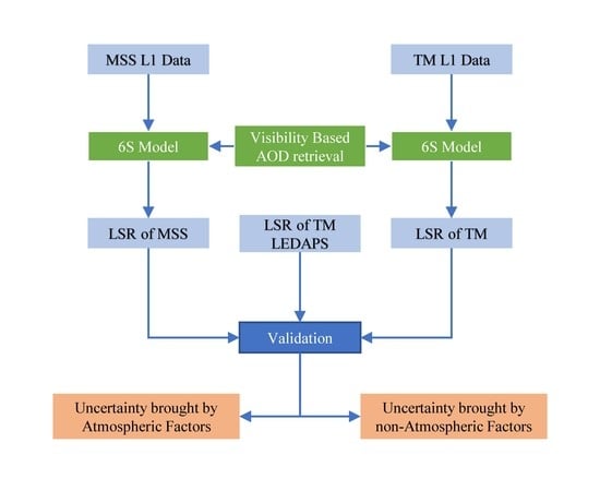
3.1. Overview
3.2. 6SV Atmospheric Correction Model
3.3. AOD Retrieval Model Based on Visibility
4. Evaluation and Uncertainty Analysis
4.1. Comparison Method
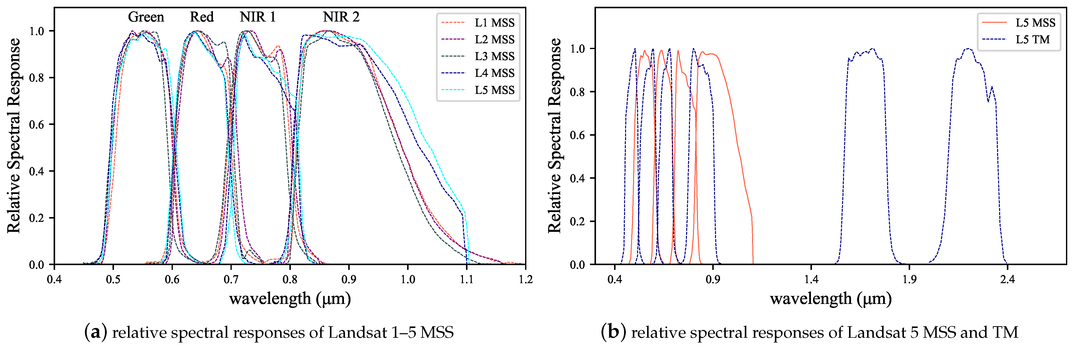
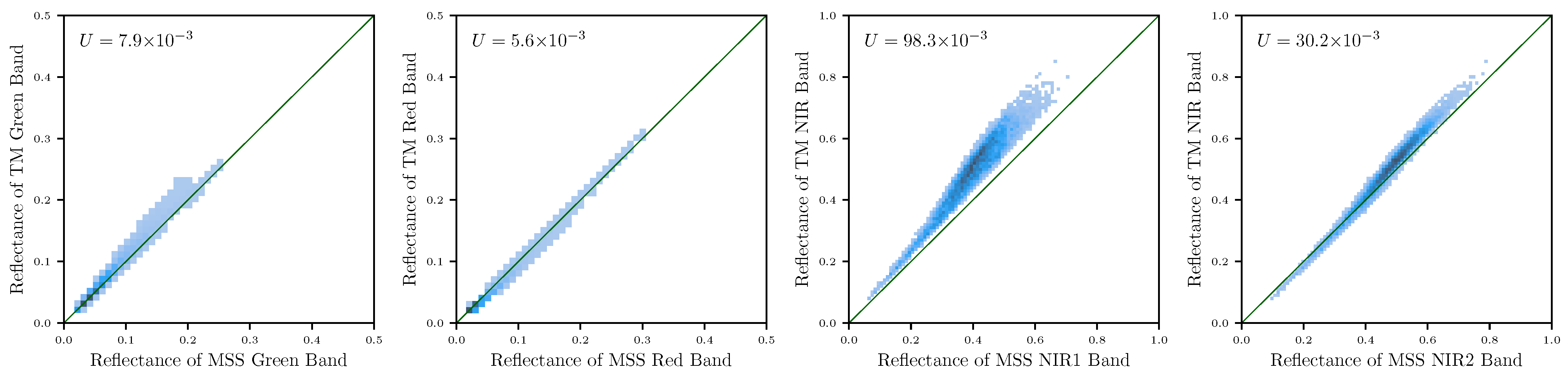
4.2. Uncertainty Brought by RSR
4.3. Uncertainty Brought by Georegistration and Scale Effects
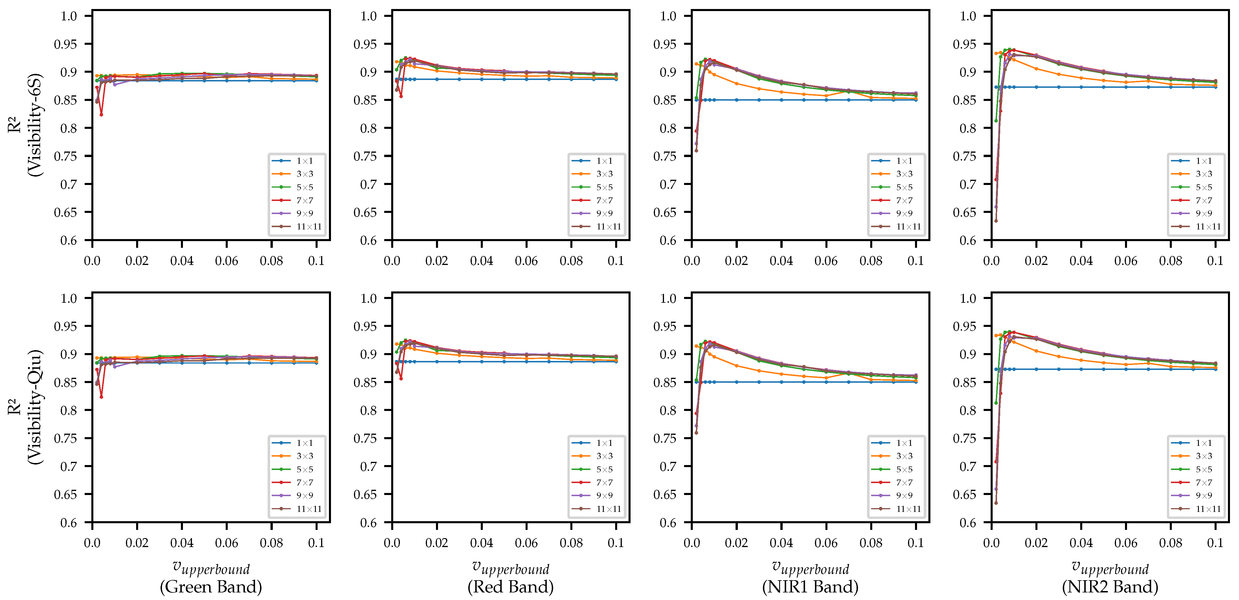
4.4. Uncertainty Brought by AOD Estimation
4.5. Other Uncertainty Sources
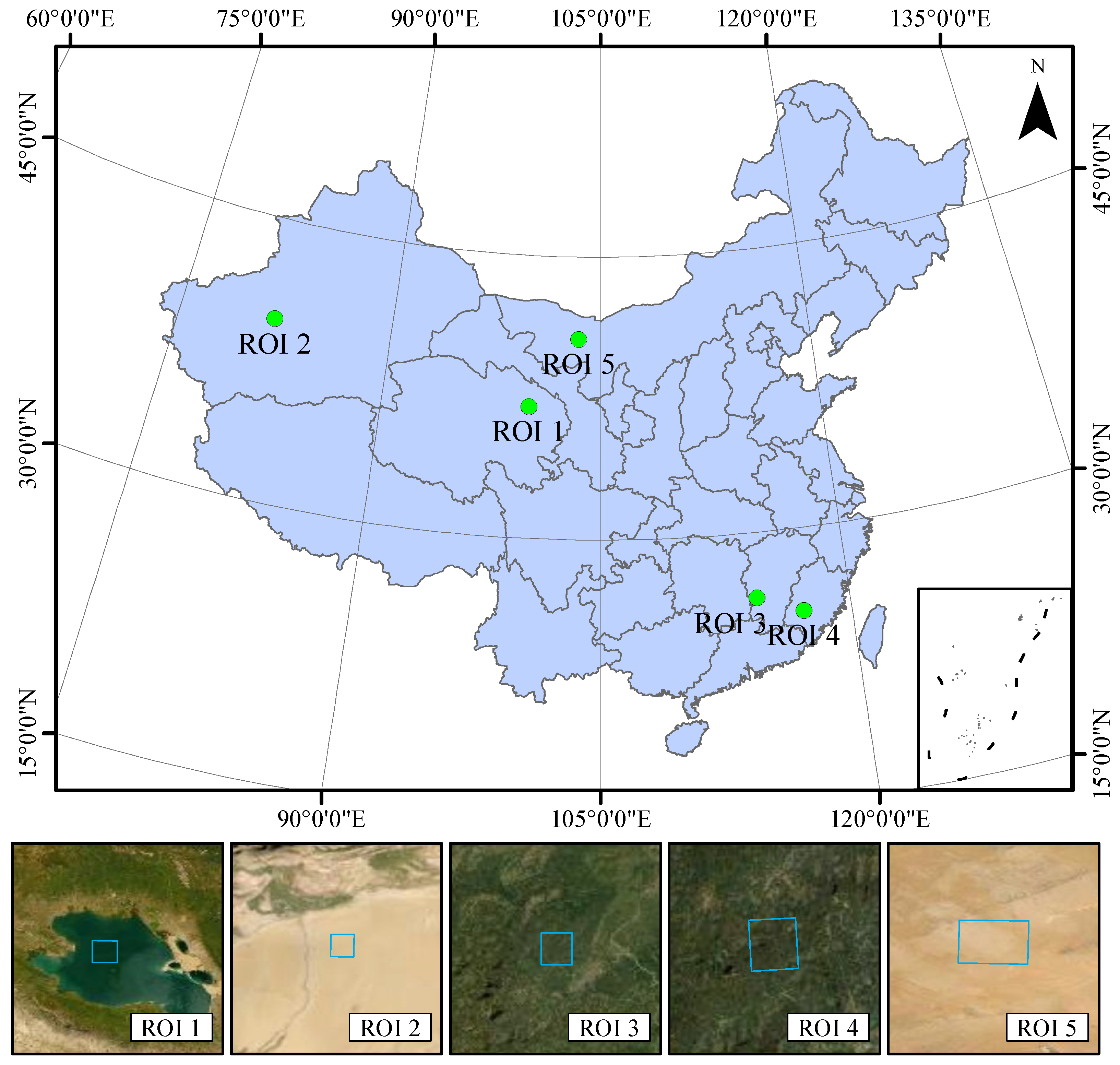
5. Application of Time-Series SR in Spectral-Stable Land Cover
5.1. Water Body
5.2. Desert
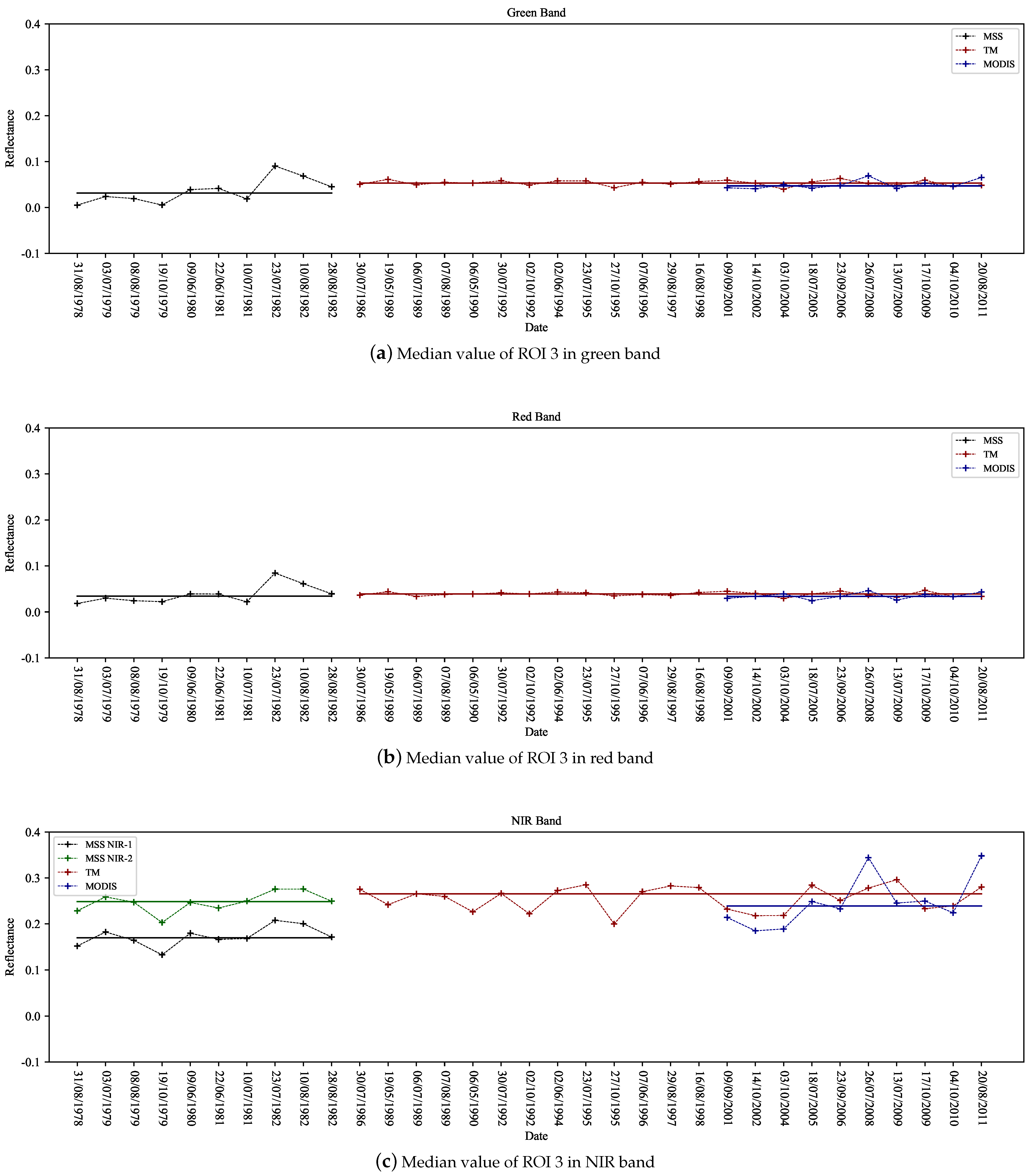
5.3. Vegetation
6. Discussion
6.1. Comparison of the Proposed Framework and LEDAPS
6.2. Analysis of Potential Problems in Time-Series Analysis of Early Years
6.3. Future Work
7. Conclusions
Author Contributions
Funding
Institutional Review Board Statement
Informed Consent Statement
Data Availability Statement
Acknowledgments
Conflicts of Interest
References
- Wulder, M.A.; Loveland, T.R.; Roy, D.P.; Crawford, C.J.; Masek, J.G.; Woodcock, C.E.; Allen, R.G.; Anderson, M.C.; Belward, A.S.; Cohen, W.B.; et al. Current Status of Landsat Program, Science, and Applications. Remote Sens. Environ. 2019, 225, 127–147. [Google Scholar] [CrossRef]
- Ju, J.; Roy, D.P.; Vermote, E.; Masek, J.; Kovalskyy, V. Continental-Scale Validation of MODIS-based and LEDAPS Landsat ETM+ Atmospheric Correction Methods. Remote Sens. Environ. 2012, 122, 175–184. [Google Scholar] [CrossRef] [Green Version]
- Claverie, M.; Vermote, E.F.; Franch, B.; Masek, J.G. Evaluation of the Landsat-5 TM and Landsat-7 ETM+ Surface Reflectance Products. Remote Sens. Environ. 2015, 169, 390–403. [Google Scholar] [CrossRef]
- Vermote, E.; Justice, C.; Claverie, M.; Franch, B. Preliminary Analysis of the Performance of the Landsat 8/OLI Land Surface Reflectance Product. Remote Sens. Environ. 2016, 185, 46–56. [Google Scholar] [CrossRef]
- Helder, D.L.; Karki, S.; Bhatt, R.; Micijevic, E.; Aaron, D.; Jasinski, B. Radiometric Calibration of the Landsat MSS Sensor Series. IEEE Trans. Geosci. Remote Sens. 2012, 50, 2380–2399. [Google Scholar] [CrossRef]
- Teixeira Pinto, C.; Haque, M.O.; Micijevic, E.; Helder, D.L. Landsats 1–5 Multispectral Scanner System Sensors Radiometric Calibration Update. IEEE Trans. Geosci. Remote Sens. 2019, 57, 7378–7394. [Google Scholar] [CrossRef]
- Gutman, G.; Huang, C.; Chander, G.; Noojipady, P.; Masek, J.G. Assessment of the NASA–USGS Global Land Survey (GLS) Datasets. Remote Sens. Environ. 2013, 134, 249–265. [Google Scholar] [CrossRef]
- Yan, L.; Roy, D. Improving Landsat Multispectral Scanner (MSS) Geolocation by Least-Squares-Adjustment Based Time-Series Co-Registration. Remote Sens. Environ. 2021, 252, 112181. [Google Scholar] [CrossRef]
- Vogeler, J.C.; Braaten, J.D.; Slesak, R.A.; Falkowski, M.J. Extracting the Full Value of the Landsat Archive: Inter-sensor Harmonization for the Mapping of Minnesota Forest Canopy Cover (1973–2015). Remote Sens. Environ. 2018, 209, 363–374. [Google Scholar] [CrossRef]
- Chen, F.; Fan, Q.; Lou, S.; Yang, L.; Wang, C.; Claverie, M.; Wang, C.; Junior, J.M.; Goncalves, W.N.; Li, J. Characterization of MSS Channel Reflectance and Derived Spectral Indices for Building Consistent Landsat 1–5 Data Record. IEEE Trans. Geosci. Remote Sens. 2020, 58, 8967–8984. [Google Scholar] [CrossRef]
- Hall, F.G.; Strebel, D.E.; Nickeson, J.E.; Goetz, S.J. Radiometric Rectification: Toward a Common Radiometric Response among Multidate, Multisensor Images. Remote Sens. Environ. 1991, 35, 11–27. [Google Scholar] [CrossRef]
- Richter, R. Atmospheric Correction of Satellite Data with Haze Removal Including a Haze/Clear Transition Region. Comput. Geosci. 1996, 22, 675–681. [Google Scholar] [CrossRef]
- Richter, R. A Spatially Adaptive Fast Atmospheric Correction Algorithm. Int. J. Remote Sens. 1996, 17, 1201–1214. [Google Scholar] [CrossRef]
- Chavez, P.S., Jr. An Improved Dark-Object Subtraction Technique for Atmospheric Scattering Correction of Multispectral Data. Remote Sens. Environ. 1988, 24, 459–479. [Google Scholar] [CrossRef]
- Chavez, P.S., Jr. Image-Based Atmospheric Corrections-Revisited and Improved. Photogramm. Eng. Remote Sens. 1996, 62, 1025–1035. [Google Scholar]
- Liang, S. Atmospheric Correction of Landsat ETM+ Land Surface Imagery—Part I: Methods. IEEE Trans. Geosci. Remote Sens. 2001, 39, 9. [Google Scholar] [CrossRef]
- Liang, S.; Fang, H.; Chen, M.; Shuey, C.J.; Walthall, C.; Daughtry, C.; Morisette, J.; Schaaf, C.; Strahler, A. Validating MODIS Land Surface Reflectance and Albedo Products: Methods and Preliminary Results. Remote Sens. Environ. 2002, 83, 149–162. [Google Scholar] [CrossRef]
- Liang, S. Quantitative Remote Sensing of Land Surfaces; John Wiley & Sons: Hoboken, NJ, USA, 2005; Volume 30. [Google Scholar]
- Berk, A.; Bernstein, L.S.; Robertson, D.C. MODTRAN: A Moderate Resolution Model for LOWTRAN; Technical Report; Spectral Sciences Inc.: Burlington, MA, USA, 1987. [Google Scholar]
- Vermote, E.; Tanre, D.; Deuze, J.; Herman, M.; Morcette, J.J. Second Simulation of the Satellite Signal in the Solar Spectrum, 6S: An Overview. IEEE Trans. Geosci. Remote Sens. 1997, 35, 675–686. [Google Scholar] [CrossRef] [Green Version]
- Holben, B.N.; Eck, T.F.; al Slutsker, I.; Tanre, D.; Buis, J.P.; Setzer, A.; Vermote, E.; Reagan, J.A.; Kaufman, Y.J.; Nakajima, T. AERONET—A Federated Instrument Network and Data Archive for Aerosol Characterization. Remote Sens. Environ. 1998, 66, 1–16. [Google Scholar] [CrossRef]
- Kaufman, Y.J.; Sendra, C. Algorithm for Automatic Atmospheric Corrections to Visible and Near-IR Satellite Imagery. Int. J. Remote Sens. 1988, 9, 1357–1381. [Google Scholar] [CrossRef]
- Teillet, P.M.; Fedosejevs, G. On the Dark Target Approach to Atmospheric Correction of Remotely Sensed Data. Can. J. Remote Sens. 1995, 21, 374–387. [Google Scholar] [CrossRef]
- Kaufman, Y.J.; Wald, A.E.; Remer, L.A.; Gao, B.C.; Li, R.R.; Flynn, L. The MODIS 2.1-/Spl Mu/m Channel-Correlation with Visible Reflectance for Use in Remote Sensing of Aerosol. IEEE Trans. Geosci. Remote Sens. 1997, 35, 1286–1298. [Google Scholar] [CrossRef]
- Liang, S.; Fallah-Adl, H.; Kalluri, S.; JáJá, J.; Kaufman, Y.J.; Townshend, J.R.G. An Operational Atmospheric Correction Algorithm for Landsat Thematic Mapper Imagery over the Land. J. Geophys. Res. Atmos. 1997, 102, 17173–17186. [Google Scholar] [CrossRef]
- Koschmieder, H. Theorie Der Horizontalen Sichtweite, Beitrage Zur Physik Der Freien Atmosphare. Meteorol. Z. 1924, 12, 3353. [Google Scholar]
- Elterman, L. Relationships between Vertical Attenuation and Surface Meteorological Range. Appl. Opt. 1970, 9, 1804–1810. [Google Scholar] [CrossRef] [PubMed]
- Friedlander, S.K. Smoke, Dust and Haze: Fundamentals of Aerosol Behavior; Wiley-Interscience: New York, NY, USA, 1977. [Google Scholar]
- Qiu, J.; Lin, Y. A Parameterization Model of Aerosol Optical Depths in China. Acta Meteorol. Sin. 2001, 3, 368–372. (In Chinese) [Google Scholar]
- Wu, J.; Luo, J.; Zhang, L.; Xia, L.; Zhao, D.; Tang, J. Improvement of Aerosol Optical Depth Retrieval Using Visibility Data in China during the Past 50 Years. J. Geophys. Res. Atmos. 2014, 119, 13370–13387. [Google Scholar] [CrossRef]
- Kessner, A.L.; Wang, J.; Levy, R.C.; Colarco, P.R. Remote Sensing of Surface Visibility from Space: A Look at the United States East Coast. Atmos. Environ. 2013, 81, 136–147. [Google Scholar] [CrossRef] [Green Version]
- He, Q.; Li, C.; Geng, F.; Zhou, G.; Gao, W.; Yu, W.; Li, Z.; Du, M. A Parameterization Scheme of Aerosol Vertical Distribution for Surface-Level Visibility Retrieval from Satellite Remote Sensing. Remote Sens. Environ. 2016, 181, 1–13. [Google Scholar] [CrossRef]
- Zhang, Z.; Wu, W.; Wei, J.; Song, Y.; Yan, X.; Zhu, L.; Wang, Q. Aerosol Optical Depth Retrieval from Visibility in China during 1973–2014. Atmos. Environ. 2017, 171, 38–48. [Google Scholar] [CrossRef]
- USGS. Landsat Collection 1 Level 1 Product Definition V2. 2019. Available online: https://prd-wret.s3-us-west-2.amazonaws.com/assets/palladium/production/atoms/files/LSDS-1656_%20Landsat_Collection1_L1_Product_Definition-v2.pdf (accessed on 3 April 2022).
- USGS. Landsat 4–7 Collection 1 (C1) Surface Reflectance (LEDAPS) Product Guide. 2020. Available online: https://prd-wret.s3.us-west-2.amazonaws.com/assets/palladium/production/atoms/files/LSDS-1370_L4-7_C1-SurfaceReflectance-LEDAPS_ProductGuide-v3.pdf (accessed on 3 April 2022).
- Maiersperger, T.; Scaramuzza, P.; Leigh, L.; Shrestha, S.; Gallo, K.; Jenkerson, C.B.; Dwyer, J.L. Characterizing LEDAPS surface reflectance products by comparisons with AERONET, field spectrometer, and MODIS data. Remote Sens. Environ. 2013, 136, 1–13. [Google Scholar] [CrossRef] [Green Version]
- Smith, A.; Lott, N.; Vose, R. The Integrated Surface Database: Recent Developments and Partnerships. Bull. Am. Meteorol. Soc. 2011, 92, 704–708. [Google Scholar] [CrossRef]
- Kalnay, E.; Kanamitsu, M.; Kistler, R.; Collins, W.; Deaven, D.; Gandin, L.; Iredell, M.; Saha, S.; White, G.; Woollen, J. The NCEP/NCAR 40-Year Reanalysis Project. Bull. Am. Meteorol. Soc. 1996, 77, 437–472. [Google Scholar] [CrossRef] [Green Version]
- Xu, X.; Liu, J.; Zhang, S.; Li, R.; Yan, C.; Wu, S. China’s Multi-Period Land Use Land Cover Remote Sensing Monitoring Data Set (CNLUCC); Resource and Environment Data Cloud Platform: Beijing, China, 2018. [Google Scholar]
- Wang, H.; Zhao, X.; Zhang, X.; Wu, D.; Du, X. Long time series land cover classification in China from 1982 to 2015 based on Bi-LSTM deep learning. Remote Sens. 2019, 11, 1639. [Google Scholar] [CrossRef] [Green Version]
- Shen, Z.; Xu, X. Influence of the Economic Efficiency of Built-Up Land (EEBL) on Urban Heat Islands (UHIs) in the Yangtze River Delta Urban Agglomeration (YRDUA). Remote Sens. 2020, 12, 3944. [Google Scholar] [CrossRef]
- Vermote, E.; Tanré, D.; Deuzé, J.L.; Herman, M.; Morcrette, J.J.; Kotchenova, S.Y. Second Simulation of a Satellite Signal in the Solar Spectrum-Vector (6SV). 6S User Guide Version 2006, 3, 1–55. [Google Scholar]
- Elterman, L. Rayleigh and Extinction Coefficients to 50 Km for the Region 0.27 μ to 0.55 μ. Appl. Opt. 1964, 3, 1139–1147. [Google Scholar] [CrossRef]
- Deirmendjian, D. Electromagnetic Scattering on Spherical Polydispersions; Technical Report; Rand Corp: Santa Monica, CA, USA, 1969. [Google Scholar]
- McClatchey, R.A. Optical Properties of the Atmosphere (Revised); Number 354, Air Force Cambridge Research Laboratories, Office of Aerospace Research: Bedford, MA, USA, 1971. [Google Scholar]
- Meerdink, S.K.; Hook, S.J.; Roberts, D.A.; Abbott, E.A. The ECOSTRESS Spectral Library Version 1.0. Remote Sens. Environ. 2019, 230, 111196. [Google Scholar] [CrossRef]
- Jacquemoud, S.; Verhoef, W.; Baret, F.; Bacour, C.; Zarco-Tejada, P.J.; Asner, G.P.; François, C.; Ustin, S.L. PROSPECT+SAIL Models: A Review of Use for Vegetation Characterization. Remote Sens. Environ. 2009, 113, S56–S66. [Google Scholar] [CrossRef]
- Chen, J.; Zhu, W. Comparing Landsat-8 and Sentinel-2 Top of Atmosphere and Surface Reflectance in High Latitude Regions: Case Study in Alaska. Geocarto Int. 2021, 1–20. [Google Scholar] [CrossRef]
- Zhang, H.K.; Roy, D.P.; Yan, L.; Li, Z.; Huang, H.; Vermote, E.; Skakun, S.; Roger, J.C. Characterization of Sentinel-2A and Landsat-8 Top of Atmosphere, Surface, and Nadir BRDF Adjusted Reflectance and NDVI Differences. Remote Sens. Environ. 2018, 215, 482–494. [Google Scholar] [CrossRef]
- Aguilar, M.Á.; Jiménez-Lao, R.; Nemmaoui, A.; Aguilar, F.J.; Koc-San, D.; Tarantino, E.; Chourak, M. Evaluation of the Consistency of Simultaneously Acquired Sentinel-2 and Landsat 8 Imagery on Plastic Covered Greenhouses. Remote Sens. 2020, 12, 2015. [Google Scholar] [CrossRef]
- Gillingham, S.S.; Flood, N.; Gill, T.K.; Mitchell, R.M. Limitations of the Dense Dark Vegetation Method for Aerosol Retrieval under Australian Conditions. Remote Sens. Lett. 2012, 3, 67–76. [Google Scholar] [CrossRef]
- Gillingham, S.; Flood, N.; Gill, T. On Determining Appropriate Aerosol Optical Depth Values for Atmospheric Correction of Satellite Imagery for Biophysical Parameter Retrieval: Requirements and Limitations under Australian Conditions. Int. J. Remote Sens. 2013, 34, 2089–2100. [Google Scholar] [CrossRef]
- Santer, R.; Ramon, D.; Vidot, J.; Dilligeard, E. A Surface Reflectance Model for Aerosol Remote Sensing over Land. Int. J. Remote Sens. 2007, 28, 737–760. [Google Scholar] [CrossRef]
- Ji, S.; Xingqi, L.; Sumin, W.; Matsumoto, R. Palaeoclimatic Changes in the Qinghai Lake Area during the Last 18,000 Years. Quat. Int. 2005, 136, 131–140. [Google Scholar] [CrossRef]
- Schmidt, G.L.; Jenkerson, C.; Masek, J.G.; Vermote, E.; Gao, F. Landsat Ecosystem Disturbance Adaptive Processing System (LEDAPS) Algorithm Description; U.S. Geological Survey: Reston, VA, USA, 2013.
- Braaten, J.D.; Cohen, W.B.; Yang, Z. Automated cloud and cloud shadow identification in Landsat MSS imagery for temperate ecosystems. Remote Sens. Environ. 2015, 169, 128–138. [Google Scholar] [CrossRef] [Green Version]
- Zhang, S.; Wu, J.; Fan, W.; Yang, Q.; Zhao, D. Review of Aerosol Optical Depth Retrieval Using Visibility Data. Earth-Sci. Rev. 2020, 200, 102986. [Google Scholar] [CrossRef]


| MSS | TM | |
|---|---|---|
| Bands | Green, red, NIR1, NIR2 | Blue, green, red, NIR, SWIR1, TIR, SWIR2 |
| Spatial resolution | 57 × 79 m (resampled to 60 m) | 30 m |
| Radiometric resolution | 6 bit (resampled to 8 bit) | 8 bit |
| Measured Value | Truth Value | RSR Difference | Radiometric Calibration | Geographical Factors | AOD/WV Estimating | Other Factors | Reference |
|---|---|---|---|---|---|---|---|
| LSR of TM (Visibility-6S and Visibility-Qiu Method) | LSR of TM (LEDAPS) | × | × | × | ○ | × | - |
| LSR of MSS (Visibility-6S and Visibility-Qiu Method) | LSR of TM (LEDAPS) | ○ | ○ | ○ | ○ | ○ | - |
| LSR of MSS (Visibility-6S and Visibility-Qiu Method) | LSR of TM (only pure pixel) (LEDAPS) | ○ | ○ | × | ○ | ○ | - |
| effective radiance or reflectance of MSS in TOA | effective radiance or reflectance of TM in TOA | ○ | × | × | × | × | Teixeira Pinto et al. [6] |
| radiance or reflectance of MSS in TOA | radiance or reflectance of TM in TOA | ○ | ○ | ○ | × | ○ | Teixeira Pinto et al. [6] |
| Parameters | Value |
|---|---|
| Solar zenith angle | uniform (0, 70) |
| Observer zenith angle | 0 |
| Relative azimuth angle | uniform (0, 360) |
| Leaf area index | uniform (0, 8) |
| Equivalent water thickiness | uniform (0, 8) |
| Chlorophyll a + b concentration | uniform (10, 80) |
| Carotenoid concentration | uniform (0, 20) |
| Dry matter content | uniform (0.002, 0.010) |
| Brown pigment | 0 |
| PSOIL | uniform (0, 1) |
| typelidf | 2 |
| LIDFa | uniform (0, 90) |
| N | uniform (0.8, 2.5) |
| Sensor | Band | N | Comparison Metrics | |||||||||||
|---|---|---|---|---|---|---|---|---|---|---|---|---|---|---|
| Visibility–6S Compared with LEDAPS (This Work) | Visibility–Qiu Compared with LEDAPS (This Work) | TM LEDAPS Compared with MODIS BRDF [3] | LEDAPS Compared with LSR Using AERONET AOD [3] | |||||||||||
| TM | Green | 479 | —0.019 | 0.005 | 0.020 | —0.025 | 0.008 | 0.029 | 0.001 | 0.009 | 0.009 | 0.0001 | 0.0054 | 0.0054 |
| Red | 479 | —0.012 | 0.004 | 0.014 | —0.016 | 0.007 | 0.021 | 0.009 | 0.01 | 0.014 | 0.0001 | 0.0041 | 0.0041 | |
| NIR | 479 | 0.003 | 0.005 | 0.009 | 0.005 | 0.008 | 0.016 | 0.005 | 0.017 | 0.017 | 0.0032 | 0.0061 | 0.0068 | |
| MSS | Green | 479 | —0.023 | 0.013 | 0.029 | —0.029 | 0.016 | 0.039 | - | - | - | - | - | - |
| Red | 479 | —0.019 | 0.015 | 0.026 | —0.023 | 0.017 | 0.032 | - | - | - | - | - | - | |
| NIR1 | 479 | —0.017 | 0.020 | 0.033 | —0.017 | 0.022 | 0.037 | - | - | - | - | - | - | |
| NIR2 | 479 | 0.008 | 0.015 | 0.023 | 0.010 | 0.016 | 0.027 | - | - | - | - | - | - | |
| Band | MSS Visibility–6S Method | MSS Visibility–Qiu Method | ||||
|---|---|---|---|---|---|---|
| Total Uncertainty | Uncertainty Brought by Atmospheric Factors | Uncertainty Brought by Non-Atmospheric Factors | Total Uncertainty | Uncertainty Brought by Atmospheric Factors | Uncertainty Brought by Non-Atmospheric Factors | |
| Green | 0.029 | 0.020 | 0.021 | 0.039 | 0.029 | 0.025 |
| Red | 0.026 | 0.014 | 0.022 | 0.032 | 0.021 | 0.025 |
| NIR1 | 0.033 | 0.009 | 0.032 | 0.037 | 0.016 | 0.033 |
| NIR2 | 0.023 | 0.009 | 0.021 | 0.027 | 0.016 | 0.022 |
| Band | Season | N | Comparison Metrics | |||||||||||
|---|---|---|---|---|---|---|---|---|---|---|---|---|---|---|
| Visibility–6S TM | Visibility–Qiu TM | Visibility–6S MSS | Visibility–Qiu MSS | |||||||||||
| A | P | U | A | P | U | A | P | U | A | P | U | |||
| Green | MAM | 167 | —0.017 | 0.003 | 0.017 | —0.020 | 0.004 | 0.022 | —0.025 | 0.013 | 0.030 | —0.028 | 0.014 | 0.035 |
| JJA | 113 | —0.013 | 0.002 | 0.014 | —0.021 | 0.003 | 0.021 | —0.019 | 0.009 | 0.022 | —0.027 | 0.009 | 0.029 | |
| SON | 123 | —0.022 | 0.004 | 0.023 | —0.035 | 0.009 | 0.038 | —0.024 | 0.011 | 0.029 | —0.037 | 0.015 | 0.044 | |
| DJF | 76 | —0.026 | 0.012 | 0.032 | —0.026 | 0.021 | 0.042 | —0.023 | 0.022 | 0.040 | —0.022 | 0.031 | 0.052 | |
| Red | MAM | 167 | —0.012 | 0.002 | 0.012 | —0.014 | 0.003 | 0.016 | —0.023 | 0.017 | 0.029 | —0.025 | 0.017 | 0.032 |
| JJA | 113 | —0.010 | 0.002 | 0.010 | —0.016 | 0.003 | 0.017 | —0.014 | 0.015 | 0.022 | —0.021 | 0.015 | 0.027 | |
| SON | 123 | —0.014 | 0.004 | 0.015 | —0.022 | 0.008 | 0.026 | —0.017 | 0.010 | 0.021 | —0.026 | 0.014 | 0.032 | |
| DJF | 76 | —0.013 | 0.010 | 0.021 | —0.011 | 0.018 | 0.032 | —0.020 | 0.018 | 0.031 | —0.018 | 0.026 | 0.041 | |
| NIR1 | MAM | 167 | 0.002 | 0.004 | 0.007 | 0.003 | 0.005 | 0.010 | —0.016 | 0.018 | 0.028 | —0.017 | 0.018 | 0.029 |
| JJA | 113 | 0.000 | 0.004 | 0.007 | 0.000 | 0.005 | 0.012 | —0.032 | 0.023 | 0.043 | —0.034 | 0.022 | 0.043 | |
| SON | 123 | 0.002 | 0.005 | 0.008 | 0.003 | 0.010 | 0.017 | —0.017 | 0.018 | 0.029 | —0.018 | 0.020 | 0.035 | |
| DJF | 76 | 0.010 | 0.012 | 0.019 | 0.018 | 0.019 | 0.032 | 0.005 | 0.023 | 0.034 | 0.012 | 0.030 | 0.046 | |
| NIR2 | MAM | 167 | - | - | - | - | - | - | 0.008 | 0.013 | 0.021 | 0.008 | 0.014 | 0.022 |
| JJA | 113 | - | - | - | - | - | - | 0.000 | 0.014 | 0.020 | —0.001 | 0.014 | 0.022 | |
| SON | 123 | - | - | - | - | - | - | 0.012 | 0.015 | 0.026 | 0.013 | 0.018 | 0.032 | |
| DJF | 76 | - | - | - | - | - | - | 0.017 | 0.018 | 0.028 | 0.025 | 0.021 | 0.037 | |
| Band | Sensor | Min | Median | Mean | Max | SD |
|---|---|---|---|---|---|---|
| Green | MSS | —0.095 | —0.008 | —0.014 | 0.007 | 0.026 |
| TM | 0.026 | 0.035 | 0.037 | 0.062 | 0.007 | |
| MODIS | 0.008 | 0.028 | 0.031 | 0.062 | 0.012 | |
| Red | MSS | —0.026 | 0.007 | 0.006 | 0.021 | 0.012 |
| TM | 0.010 | 0.018 | 0.019 | 0.048 | 0.006 | |
| MODIS | —0.010 | 0.005 | 0.006 | 0.026 | 0.006 | |
| NIR | MSS-NIR1 | 0.000 | 0.009 | 0.010 | 0.025 | 0.007 |
| MSS-NIR2 | 0.002 | 0.014 | 0.015 | 0.029 | 0.008 | |
| TM | 0.006 | 0.013 | 0.015 | 0.044 | 0.006 | |
| MODIS | —0.010 | 0.000 | 0.001 | 0.021 | 0.005 |
| Band | Sensor | Min | Median | Mean | Max | SD |
|---|---|---|---|---|---|---|
| Green | MSS | 0.211 | 0.237 | 0.236 | 0.275 | 0.020 |
| TM | 0.213 | 0.247 | 0.247 | 0.282 | 0.015 | |
| MODIS | 0.211 | 0.228 | 0.230 | 0.282 | 0.014 | |
| Red | MSS | 0.271 | 0.298 | 0.296 | 0.312 | 0.012 |
| TM | 0.262 | 0.295 | 0.294 | 0.322 | 0.012 | |
| MODIS | 0.265 | 0.287 | 0.289 | 0.345 | 0.016 | |
| NIR | MSS NIR-1 | 0.291 | 0.328 | 0.326 | 0.346 | 0.016 |
| MSS NIR-2 | 0.289 | 0.339 | 0.333 | 0.362 | 0.018 | |
| TM | 0.292 | 0.316 | 0.316 | 0.347 | 0.010 | |
| MODIS | 0.290 | 0.314 | 0.315 | 0.369 | 0.016 |
| Band | Sensor | Min | Median | Mean | Max | SD |
|---|---|---|---|---|---|---|
| Green | MSS | 0.158 | 0.184 | 0.183 | 0.208 | 0.017 |
| TM | 0.208 | 0.232 | 0.231 | 0.271 | 0.009 | |
| MODIS | 0.178 | 0.209 | 0.207 | 0.222 | 0.010 | |
| Red | MSS | 0.252 | 0.283 | 0.281 | 0.315 | 0.017 |
| TM | 0.274 | 0.298 | 0.298 | 0.333 | 0.010 | |
| MODIS | 0.248 | 0.293 | 0.290 | 0.312 | 0.014 | |
| NIR | MSS NIR-1 | 0.302 | 0.344 | 0.339 | 0.373 | 0.019 |
| MSS NIR-2 | 0.318 | 0.364 | 0.361 | 0.392 | 0.025 | |
| TM | 0.306 | 0.335 | 0.335 | 0.365 | 0.009 | |
| MODIS | 0.296 | 0.345 | 0.341 | 0.370 | 0.015 |
| Band | Sensor | Min | Median | Mean | Max | SD |
|---|---|---|---|---|---|---|
| Green | MSS | 0.005 | 0.032 | 0.036 | 0.090 | 0.026 |
| TM | 0.040 | 0.053 | 0.053 | 0.063 | 0.006 | |
| MODIS | 0.041 | 0.047 | 0.050 | 0.069 | 0.009 | |
| Red | MSS | 0.018 | 0.034 | 0.038 | 0.085 | 0.020 |
| TM | 0.030 | 0.039 | 0.039 | 0.047 | 0.005 | |
| MODIS | 0.025 | 0.034 | 0.035 | 0.046 | 0.007 | |
| NIR | MSS NIR-1 | 0.133 | 0.170 | 0.173 | 0.208 | 0.021 |
| MSS NIR-2 | 0.203 | 0.248 | 0.247 | 0.276 | 0.021 | |
| TM | 0.200 | 0.266 | 0.256 | 0.296 | 0.027 | |
| MODIS | 0.185 | 0.239 | 0.248 | 0.348 | 0.054 |
| Band | Sensor | Min | Median | Mean | Max | SD |
|---|---|---|---|---|---|---|
| Green | MSS | —0.007 | 0.019 | 0.022 | 0.070 | 0.023 |
| TM | 0.032 | 0.047 | 0.049 | 0.070 | 0.009 | |
| MODIS | 0.037 | 0.051 | 0.053 | 0.072 | 0.011 | |
| Red | MSS | 0.016 | 0.030 | 0.035 | 0.072 | 0.016 |
| TM | 0.024 | 0.034 | 0.037 | 0.057 | 0.008 | |
| MODIS | 0.026 | 0.034 | 0.037 | 0.059 | 0.009 | |
| NIR | MSS NIR-1 | 0.115 | 0.160 | 0.153 | 0.188 | 0.020 |
| MSS NIR-2 | 0.154 | 0.240 | 0.228 | 0.275 | 0.037 | |
| TM | 0.175 | 0.231 | 0.234 | 0.276 | 0.027 | |
| MODIS | 0.194 | 0.271 | 0.263 | 0.329 | 0.040 |
Publisher’s Note: MDPI stays neutral with regard to jurisdictional claims in published maps and institutional affiliations. |
© 2022 by the authors. Licensee MDPI, Basel, Switzerland. This article is an open access article distributed under the terms and conditions of the Creative Commons Attribution (CC BY) license (https://creativecommons.org/licenses/by/4.0/).
Share and Cite
Zhao, C.; Wu, Z.; Qin, Q.; Ye, X. A Framework of Generating Land Surface Reflectance of China Early Landsat MSS Images by Visibility Data and Its Evaluation. Remote Sens. 2022, 14, 1802. https://doi.org/10.3390/rs14081802
Zhao C, Wu Z, Qin Q, Ye X. A Framework of Generating Land Surface Reflectance of China Early Landsat MSS Images by Visibility Data and Its Evaluation. Remote Sensing. 2022; 14(8):1802. https://doi.org/10.3390/rs14081802
Chicago/Turabian StyleZhao, Cong, Zihua Wu, Qiming Qin, and Xin Ye. 2022. "A Framework of Generating Land Surface Reflectance of China Early Landsat MSS Images by Visibility Data and Its Evaluation" Remote Sensing 14, no. 8: 1802. https://doi.org/10.3390/rs14081802