A New Method for Retrieving Electron Density Profiles from the MARSIS Ionograms

Abstract

The Martian ionosphere was actively detected by Mars Advanced Radar for Subsurface and Ionosphere Sounding (MARSIS) aboard the Mars Express. The detected echo signal of the MARSIS at an epoch is presented as a function of frequency and time delay to form an ionogram. Some MARSIS ionograms have been processed to obtain the electron density profiles of the Martian topside ionosphere. Unfortunately, more than half of the records cannot be processed with current methods due to the lack of local plasma density information at spacecraft altitude. In this work, we employ a piece-wise exponent to describe the electron density profile of the Martian topside ionosphere. The piece-wise exponent used in our method can reasonably capture the altitude structure of the Martian topside ionosphere, which has been validated with the MGS and MAVEN data. In an altitude regime of lower than 200 km, the average absolute height error of the same electron density between MGS data and fitted profiles is 0.006 km, and the average relative error is 0.008%. In an altitude regime of higher than 200 km, the average absolute height error of the same electron density between MGS data and fitted profiles is 0.55 km, and the average relative error is −0.1%. Based on the altitude structure knowledge of the Martian topside ionosphere, we put forward a new method to invert electron density profiles from MARSIS ionograms with/without local plasma density information. Compared with the previous results, the average absolute difference in the peak height of the retrieved profile is 7.38 km, within the margin of the MARSIS height resolution of 13.8 km. The average relative difference is only 3%. The application of the new method can greatly improve the utilization rate of MARSIS ionogram records.

1. Introduction

Since the existence of the Earth’s ionosphere has been experimentally proven, a large number of scientists have achieved many outstanding results [1,2,3]. With the in-depth understanding of the earth’s ionosphere and the development of science and technology, the study of the ionosphere has gradually extended from Earth to various planets. As two terrestrial planets with atmospheres, the ionospheres of Venus and Mars have been widely studied [4]. Taking Mars as an example, the detection of the Martian ionosphere can be traced back to the Martian flyby of the Mariner in 1965 [5]. More and more exploration missions have been launched to explore Mars. Among them, ionospheric measurements from missions are widely used, such as the Mars Global Surveyor (MGS), Mars Atmosphere and Volatile Evolution (MAVEN), and Mars Express (MEX).

These three missions adopted different techniques to measure the Martian ionosphere [6]. MGS probed the Martian ionosphere using the radio occultation technique. MGS accumulated a total of 5600 electron density profiles in seven years [7]. The instruments carried on MAVEN provide more comprehensive information about charged particles of the Martian ionosphere by in situ detection, such as Neutral Gas and Ion Mass Spectrometer (NGIMS), radio science ROSE, and the Langmuir probe [8]. The Mars Advanced Radar for Subsurface and Ionosphere Sounding (MARSIS) instrument carried out on MEX can actively explore the Martian ionosphere by radar detection, and the Mars Radio Science Experiment (MaRS) instrument carried out on MEX also uses the radio occultation techniques to measure the Martian ionosphere [9,10,11]. Among them, the accumulated MARSIS data have provided a potential data resource for the study of the Martian ionosphere since 2005.

As we know, different detection techniques have inherent advantages and disadvantages [6]. Detection with radio occultation is limited by the relative geometry of Earth and Mars. As a result, the solar zenith angle of the electron density profiles obtained by MGS is constrained within the range of 70°–90° [12]. The in situ detection adopted by MAVEN provides in situ plasma and neutral measurements, but cannot provide simultaneous altitudinal profiles at the same epoch. In contrast, MARSIS data cover almost all zenith angles, latitudes, and longitudes. MARSIS thus has an outstandingly high spatial and temporal resolution. The fly in the ointment is that radar detection cannot prospect the ionosphere below the peak height. Anyway, these data are of great significance for our study of the Martian ionosphere. Electron/ion density profiles of the Martian ionosphere measured by the MGS and MAVEN are publicly available from the website. However, publicly accessible MARSIS data are only original ionogram records. The electron density profiles retrieved from the MARSIS ionogram records are not open access. Effort is required to deal with the high number of MARSIS records.

The reported MARSIS data-processing method is the lamination method proposed by Morgan et al. [13,14]. Alternatively, Gurnett et al. [15] used the analytical inversion of Abel’s integral equation to retrieved electron density profiles from MARSIS ionograms in terms of an analytical expression. Later, Zou et al. [16] designed an inversion method to obtain information on electron density in the valley regions. After constructing empirical orthogonal functions (EOF) using MGS data, Han and Wan [17] adopted the EOF series to invert the density profiles. All these methods require information on the local plasma density at the Mars Express altitude. Unfortunately, a high number of ionograms cannot provide the required local plasma frequency at spacecraft altitude for various reasons [18]. For those ionograms, such traditional methods [14,15,16,17] cannot retrieve electron density profiles.

In this paper, we propose a new method for processing MARSIS ionograms with/without local plasma frequency. The method assumes that the topside ionosphere of Mars can be described in terms of piece-wise exponents. The piece-wise exponent functions are validated with the available MGS and MAVEN data. A comparison is made of the electron density profiles retrieved with our method with those of Morgan et al. [14]. The results indicate that our method can retrieve reliable electron density profiles from ionograms recorded by MARSIS, regardless of the presence or absence of local plasma density oscillation.

2. Data and Methodology

2.1. MARSIS Data Presentation and Preliminary Processing

The MARSIS is a low-frequency, pulse-limited radar, which uses synthetic aperture techniques onboard Mars Express. The operation of MARSIS has two modes: active Ionospheric detection (AIS) mode and subsurface sounding modes [11]. When Mars Express dropped lower than 1200 km, the AIS mode began to work. Radio waves with 160 ununiform frequencies from 0.1 to 5.5 MHz were transmitted to detect the ionosphere in the AIS mode.

According to the Appleton-Hartree (A-H) formula [19], when the radar detection radio wave frequency reaches the plasma frequency at the corresponding height, the radio wave will be reflected by the ionosphere plasma. The radar can detect the time delay and intensity of the reflected signal at the corresponding frequencies. MARSIS data are ionograms, which graphically display the reflection echo intensity as a function of radio wave frequency and time delay (or apparent range). The virtual height of an echo means the distance between the ground and the point at which the radio wave is reflected. The virtual height can be determined from the difference in the altitude of the spacecraft and the apparent range. An ionogram contains a lot of information about the Martian ionosphere, including its ionospheric echo, oblique ionospheric echo, surface reflection, electron cyclotron echoes, electron plasma oscillation, etc. [14]. Among these, the existence of electron plasma oscillation indicates the plasma frequency at the spacecraft altitude, and ionospheric echoes represent the plasma frequency at different heights of the Martian topside ionosphere. These are the most important information for us.

MARSIS observations offer more than 1.8 million ionograms during the MEX mission.

Figure 1 displays two typical ionograms recorded by MARSIS. Figure 1a depicts an example of MARSIS ionogram-recorded local plasma oscillation at spacecraft altitude and ionospheric echoes. The local plasma oscillation signals are absent in other kinds of ionogram, as shown in Figure 1b.

We randomly selected 10,000 ionograms for statistical analysis in the range of orbit from 1844 to 4799. In the selected 10,000 ionograms, 4940 ionograms had a discernable trace of ionospheric echoes, while 5060 ionograms had no identifiable trace of ionospheric echoes. Among the 4940 ionograms, 2072 ionograms had both local electron plasma oscillation and ionospheric echoes, and 2868 ionograms had only ionospheric echoes while missing local plasma oscillations. This indicates that more than half of the MARSIS ionograms have no local plasma frequency information.

The procedure of scaling ionograms is introduced as follows. Firstly, ionograms are displayed one by one on the screen. Secondly, the cursor is moved to select the center of the ionospheric echoes on the ionograms. The corresponding frequency and apparent range of the selected point are assigned to variables. Thirdly, the selected points are interpolated to the unpicked points between the maximum and minimum frequencies. If there are traces of local plasma oscillation, they will be scaled and extracted using the method of Morgan et al. [14]. Finally, information on the scaled trace contained in an ionogram is stored in a file for further processing.

2.2. Method of Retrieving Electron Density Profiles from MARSIS Ionogram

There are several ways to retrieve electron density profiles from the MARSIS ionograms. The most popular method is the lamination method adopted by Morgan et al. [14]. They took the spacecraft altitude and local plasma frequency extracted from plasma oscillations in the ionogram as known information. An exponential function is used to describe the relationship between plasma density or plasma frequency and height in the interval between two points in a scaled trace.

Assuming N points of the trace are being scaled from an ionogram, and counting the points from 0 to N − 1 with increasing frequency, Equation (1) describes the general function of plasma frequency $f_p$ versus height $z$ in the $j$ height interval.

$$f_p\left(z\right)=f_{s,j-1}\exp \left({\alpha }_{j}z\right)$$

(1)

where ${\alpha }_j$is the exponential growth constant of plasma frequency in the $j$ height interval. In this interval, $f_{s,j-1}\le f_p\le f_{s,j}$. $f_{s,j-1}$ is the transmitting radio frequency at the beginning of the $j$ interval, and $f_{s,j}$ is the transmitting radio frequency at the end of the $j$ interval. The apparent range of echoes contains the information of the electron density profile through which the radio wave propagates. According to the A-H theory of radio wave propagation, N − 1 equations can be constructed from the scaled N points [14].

In the equation set, there are N variables of plasma frequency. In Morgan et al. [13], when the local plasma oscillation provides information for point 0 (the spacecraft altitude), the equation set can be simultaneously resolved to obtain a set of N − 1 ${\alpha }_j$. As mentioned, the above solution requires local plasma frequency at spacecraft altitude. When this is missing, as is the case in Figure 1b, the ionogram cannot provide an electron density profile with the method of Morgan et al. [14].

Our goal was to develop a method to retrieve electron density profiles from the MARSIS ionograms when they miss local plasma oscillations. Firstly, we must adopt a function to describe the electron density profile of the Martian ionosphere as accurately as possible. In this work, we supposed that every five frequency points fits an exponential function according to Equation (2).

$$f_p\left(h\right)=f_{s,j+4}exp\left[{\alpha }_j\ast \left(h-h_{j+4}\right)\right] \left(h>h_{j+4}\right)$$

(2)

where ${\alpha }_j$is the constant of exponential growth in the $j$ interval. In the $j$ interval, $f_p\le f_{s,j+4}$. $f_{s,j+4}$ is the emission frequency at the lower end of the height interval. $h_{j+4}$ is attitude of $f_{s,j+4}$.

When the information on plasma frequency at spacecraft height is absent, there are two unknown parameters, $h_{j+4}$ and ${\alpha }_j$, in the first five frequencies points. Under the two given parameters $h_{j+4\_0}$ and ${\alpha }_{j\_0}$, we can acquire an electron density profile, and obtain the trace by processing the current electron density profile through the A-H formula. Then, the objective function of the calculated trace and the scaled trace can be constructed, as in Equation (3).

$$error=\frac{1}{M}{\displaystyle \sum }_{i=1}^M\left|\frac{T_i^{\prime }-T_i}{T_i}\right|$$

(3)

where M is the number of the points; in our method, M is 5. T is the array of scaled trace points given to or extracted from the MARSIS ionogram. This is known information. T_i is the i point of the scaled trace. T′ is the array of calculated trace points by given parameters $h_{j+4}$ and ${\alpha }_j$. $T_i^{\prime }$ is the $i$ point of the calculated trace. A nonlinear equation can be established by combining Equations (2) and (3).

$$\mathrm{y}(h_{j+4},{\alpha }_j)\to 0$$

(4)

This can be solved by using the Nelder—Mead algorithm iteration for the initial value [20]. The parameter values corresponding to the minimum value of the function are built, which are the best parameters. Then, an electron density profile of the first five frequency points can be built from the obtained parameters.

In the next five frequency points, the height of the first frequency is already known. When the initial value of $h_{j+4\_0}$ is given, ${\alpha }_{j\_0}$ can be calculated by Equation (5):

$${\alpha }_{j\_0}=\ln \left(\frac{f_{pj}}{f_{pj+4\_0}}\right)/\left(h_j-h_{j+4\_0}\right)$$

(5)

According to A-H formula, the trace can be obtained by processing the current electron density profile which calculated by $h_{j+4\_0}$ and ${\alpha }_{j\_0}$. Equation (3) also can be established. Different from the first step, there is only one parameter that needs to be fitted. The nonlinear equation is:

$$y\left(h_{j+4}\right)\to 0$$

(6)

The parameter can be calculated by the Nelder—Mead algorithm iteration. Then, the electron density profile of the second five frequencies can be obtained. After that, all frequency points can be completed step by step with the procedure mentioned above.

When information on local plasma frequency at spacecraft height is available, it is equivalent to the case where the first step in the above method has been completed. We can directly use the second step to conduct the inversion of all frequency points. Above all, our method can not only deal with the ionograms without local plasma oscillation but also those with information on local plasma frequency at spacecraft height.

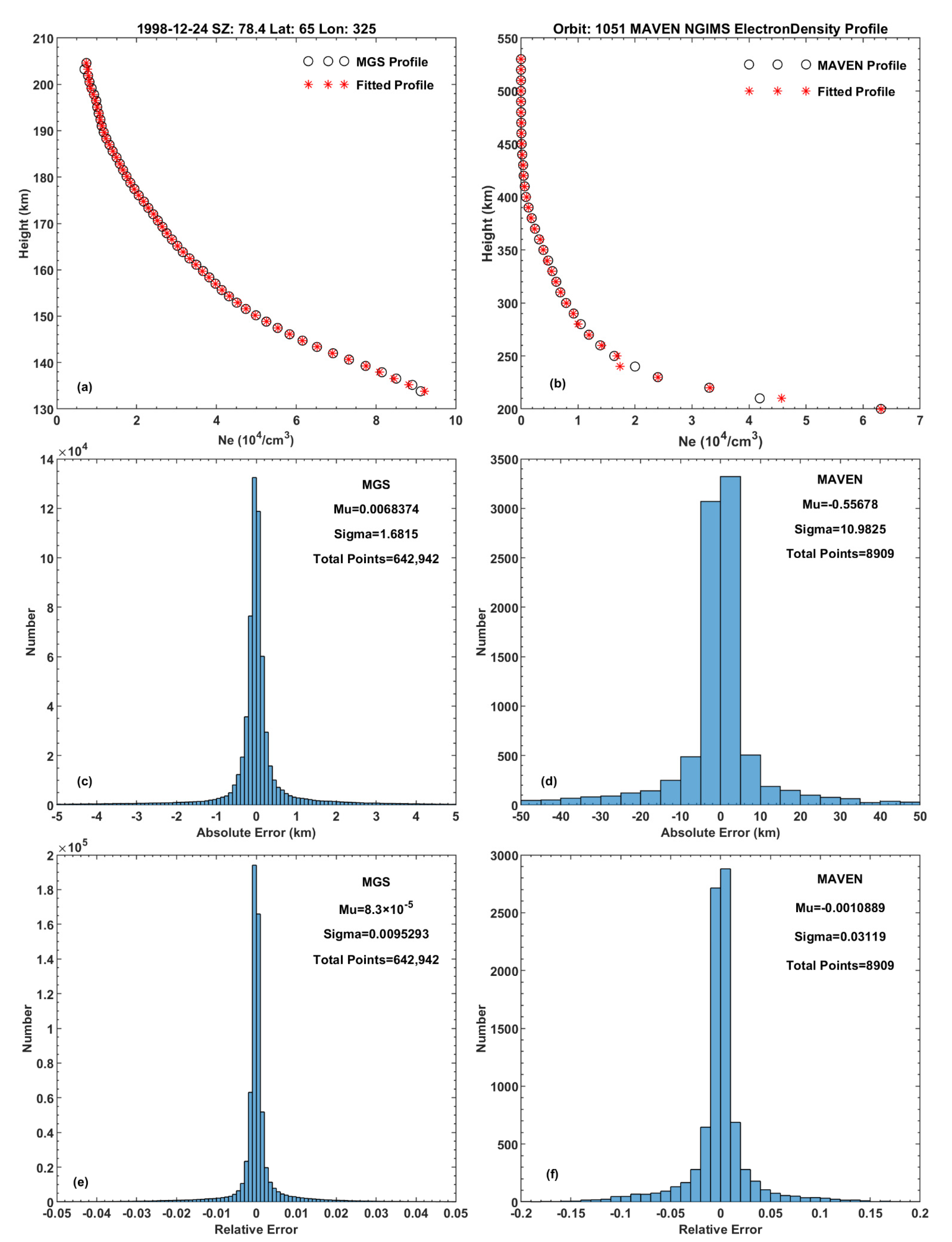
3. Validation of the Profile Expression and Inversion Method

In the method, a piece-wise exponent function was adapted to describe the Martian topside ionosphere. This assumption can be validated with the data of 5600 profiles from MGS and 701 orbits of MAVEN. The statistical comparisons between the piece-wise exponent function and observed data are shown in Figure 2.

Figure 2 displays that the errors between the fitted profile and the profile from MGS and MAVEN are almost negligible. In the altitude regime of lower than 200 km, the average absolute height error of the same electron density is 0.006 km, and the average relative error is 8.3 × 10⁻⁵. In the altitude regime of higher than 200 km, the average absolute height error of the same electron density is −0.55 km, and the average relative error is −0.001. This is much smaller than the range resolution of MARSIS [14]. This indicates that a piece-wise exponential function can accurately describe the Martian topside ionosphere for our purpose.

Then, we verified the accuracy of our retrieval method. Firstly, the A-H formula was used to process the given ideal model (piece-wise exponential electron density profile) and to obtain a trace with the same frequency as the ionospheric echo scaled from the MARSIS ionograms. Secondly, we regarded the trace obtained in the first step as the available information and used our method for inversion. Finally, the retrieved electron density profile was compared with the given ideal model. The results are illustrated in Figure 3.

In Figure 3a,b, the retrieved profile and fitted trace are almost identical to the given profile and trace in the top and middle panels. The absolute deviations between our result and real profile are in the range of from −1 to 1 km, and the relative deviation approaches 0, as shown in the bottom panel. The difference between the two pictures is almost negligible. Errors are within acceptable range whether local information is used or not. This supports that our method has potential application for processing the ionograms.

4. Performance of Our Method

The feasibility of our method has been demonstrated in Section 3. Now, the method is applied to deal with the MARSIS ionograms. Figure 4 displays the retrieved electron density profile from ionograms with (left)/without (right) information on local plasma frequency at spacecraft height. Figure 4a,b are the selected ionograms. The left panel has information on local plasma frequency at spacecraft height and the right does not. The scaled trace from selected ionograms and fitted trace by our method are shown in Figure 4c,d. They have a good consistency. Figure 4e,f show the electron density profile retrieved from the ionograms. The left panel has two profiles, retrieved by our method and Morgan’s method, respectively. It is revealed that our result is similar to Morgan’s result when the local information is available. Only one electron density profile was retrieved by our method in the right because Morgan’s method cannot retrieve the electron density profile without information on local plasma frequency at spacecraft height.

Next, the aim was to confirm how much the profiles obtained by our method deviate from the real profiles in the absence of local information. Morgan’s results are considered to be close to the real profiles. A total of 167 MARSIS ionograms with local information were selected; one of them is shown in Figure 5a. Then, the electron density profiles were retrieved using Morgan’s method and our method without using local information, respectively. The comparison is shown in Figure 5b. It is worth noting that the figure only shows the profile in the range of scaled trace. This is for two reasons. Firstly, results beyond the range of the scaled trace may be incorrect without the limitations of local information. Secondly, the low-frequency region has less influence on electromagnetic waves’ propagation. We still retrieved the local plasma frequency for this case using our method. The inferred local plasma frequency is 0.21 MHz, which is slightly lower than the real value of 0.24 Mhz. In the top panel, the trends for our profile and Morgan’s profile are consistent. However, our profile is lower than Morgan’s profile at all altitudes, which may be due to the difference in local plasma frequency. In the middle panel, the fitted trace is also nearly coincident with the scaled trace. In the bottom panel, the absolute deviation between our profile and Morgan’s profile ranges from −5 to −10 km, which is less than the MARSIS height resolution of 13.8 km. The relative deviation ranges from 2% to 4%. Figure 5c,d display statistical comparisons of 167 MARSIS ionograms. The average absolute error between our profiles and Morgan’s profiles is 7.38 km, which is within the MARSIS height resolution margin of 13.8 km. The average relative error is only 3%. It is revealed that our method can invert the ionospheric electron density profiles of Martian topside ionosphere from MARSIS ionograms without information at spacecraft altitude in the range of scaled trace.

5. Discussion

Ionogram processing methods have been developed since the 1930s. The original method was proposed by Whittaker and Watson [21]. To date, dozens of inversion methods have been proposed. They can be divided into two categories: model methods and integral equation methods [22]. In the model method, it is assumed that the real height–electron density distribution satisfies a specific model. When the ionograms obtained by the model are made to be consistent with the existing ionograms by modifying the parameters, the ionospheric information can be obtained [23]. The integral equation method is to find the analytical expression of the electron density distribution using mathematical methods. As the virtual height-electron density profile of the ionograms is discontinuous and not smooth, it is difficult to obtain an accurate solution using the direct analytical method. Therefore, in practical applications, lamination and polynomial analysis methods are usually used. Lamination assumes that the ionosphere is layered horizontally. The real height of the electron density profile is calculated from the lowest frequency. This is calculated by fitting the imaginary height using the refractive index of the ionosphere, and in each step, the calculation begins at the real height determined in the previous step. The polynomial analysis method assumes that the distribution of electron density with height can be represented by a polynomial or a modified polynomial function. Many scientists have carried out related work on the above methods. Some representative works have been listed in

Table 1. Methods for ionogram inversion [21,22,23,24,25,26,27,28,29,30,31,32,33,34,35,36,37,38,39,40,41,42,43,44,45,46,47,48,49,50,51,52,53,54,55,56].

Model Method	Integral Equation Method
	Direct	Lamination	Polynomial
Parabolic N(h) Appleton and Beynon (1940) Booker and Seaton (1940) Ratcliffe (1951a) Beynon and Thomas (1956) Chapman N(h) Pierce (1947) Other Distributions N(h) Appleton (1928, 1930) Ratcliffe (1951b) Shin and Whale (1952) Shinn (1953)	Appleton (1930) De Groot (1930) Manning (1947) Kelso (1952) Rydbeck (1942) Kelso (1954, 1957) Schemrling (1958) Whale (1951)	Murray and Hong (1937) King (1954) Jackson (1956) Titheridge (1975) Schmerling (1957) Thomas, Haselgrove, and Robbins (1958) Thomas and Vickers (1959) Titheridge (1979)	Titheridge (1961, 1967, 1969, 1986, 1988) Titheridge and Lobb (1977) Huang and Reinisch (1982) Ding et al. (2007)

.

Both methods have their strengths and weaknesses. Morgan et al. [14], Gurrent et al. [15], and Zou et al. [16] utilized the integral equation method. The integral equation method can make full use of the existing information and obtain a unique solution under certain assumptions. Therefore, it requires high data accuracy and local plasma frequency for the spacecraft as the starting point of the calculation. Our method belongs to the model method. The solution of this method is approximate. It depends on the difference between the model we chose and the real ionosphere structure.

For the Earth’s topside ionosphere, a variety of ionosphere models have been proposed. One of the most typical is the Chapman model. Many scholars have optimized this and proposed new models. Kutiev et al. [57,58,59] and Belehaki et al. [60] proposed a model that uses the Chapman profile for low altitudes and an exponential function for high altitudes. Luan et al. [61] and Liu et al. [62] adopted the Chapman function with a linearly varying scale height with altitude. Zhu et al. [63] developed a model that uses the Chapman function with a fixed scale height for low altitudes, and the Chapman function with varying scale heights for high altitudes. In addition, Reinisch et al. [64], Coїsson et al. [65], and Nava et al. [66] also proposed other forms of models of the topside ionosphere.

For Mars, only the Chapman model is used to describe the Martian topside ionosphere. Few new models were provided to represent the Martian topside ionosphere. Thus, there are only a few works on processing MARSIS ionograms using the model method. Gurrent et al. [67] performed a preliminary fitting of the Martian ionosphere using the Chapman model, but only for low heights. We choose a piece-wise exponential function to describe the Martian topside ionosphere and utilized it to handle MARSIS ionograms. Our method is a promising approach to processing MARSIS ionograms. Piece-wise exponential function is a simple and easy-to-calculate form for portraying Martian topside ionosphere. It is foreseeable that a more refined model of the Martian topside ionosphere can be adopted to process the MARSIS ionograms. Furthermore, it can also be used in other planetary topside sounding missions.

6. Conclusions

We use a piece-wise exponential to describe the Martian topside ionosphere. This assumption was verified by observations of the electron density profiles from MGS and MAVEN. The validation reveals that the piece-wise exponential function can depict the Martian topside ionosphere. We further propose a new method to invert MARSIS ionograms. One of the outstanding features of our method is that it can retrieve reliable electron density profiles from ionograms recorded by MARSIS, regardless of the presence or absence of local plasma density oscillation. Compared with previous methods, the results are within an acceptable error range. It is expected that our method will greatly improve data utilization in future MARSIS ionogram processing. Moreover, it also has potential applications in other planetary topside sounding missions.

References

1. Chapman, S. The absorption and dissociative or ionizing effect of monochromatic radiation in an atmosphere on a rotating Earth. Proc. Phys. Soc. 1931, 43, 26–45. [Google Scholar] [CrossRef]
2. Appleton, E.V.; Barnett, M.A.F. On some direct evidence for downward atmospheric reflection of electric rays. Proc. Phys. Soc. 1925, 109, 621. [Google Scholar] [CrossRef]
3. Breit, G.; Tuve, M.A. A test of the existence of the conducting layer. Phys. Rev. 1926, 28, 554. [Google Scholar] [CrossRef]
4. Cao, Y.T.; Niu, D.D.; Cui, J.; Wu, X.S. Review of Venusian and Martian ionospheres. Rev. Geophys. Planet. Phys. 2021, 52, 528–542. [Google Scholar] [CrossRef]
5. Luhmann, J.G.; Russell, C.T.; Brace, L.H.; Vaisberg, O.L. The intrinsic magnetic field and solar-wind interaction of Mars. Mars 1992, 1, 1090–1134. [Google Scholar] [CrossRef]
6. Zou, H.; Chen, H.F.; Shi, W.H. Detection of Martian ionosphere. Chin. J. Space Sci. 2011, 31, 323–332. [Google Scholar]
7. Hinson, D.P.; Tyler, G.L.; Hoilingsworth, J.L. Radio Occultation Measurements of Forced Atmospheric Waves on Mars. J. Geophys. Res. 2001, 106, 1463. [Google Scholar] [CrossRef]
8. Benna, M.; Mahaffy, P.R.; Grebowsky, J.M. First measurements of composition and dynamics of the Martian ionosphere by MAVEN’s neutral gas and ion mass spectrometer. Geophys. Res. Lett. 2015, 42, 8958–8965. [Google Scholar] [CrossRef] [Green Version]
9. Chicarro, A.; Martin, P.; Trautner, R. Mars Express: A European Mission to the Red Planet, 1st ed.; European Space Agency Publication Division: Noordwijk, The Netherlands, 2004. [Google Scholar]
10. Picardi, G.; Sorge, S.; Seu, R.; Plaut, J.; Johnson, W.; Jordan, R.; Gurnett, D.; Orosei, R.; Borgarelli, L.; Braconi, G. The Mars advanced radar for subsurface and ionosphere sounding (MARSIS): Concept and performance. In Proceedings of the Geoscience and Remote Sensing Symposium, Humburg, Germany, 28 June–2 July 1999; Volume 5, pp. 2674–2677. [Google Scholar] [CrossRef]
11. Jordan, R.; Picardi, G.; Plaut, J. The Mars Express MARSIS sounder instrument. Planet. Space Sci. 2009, 57, 1975–1986. [Google Scholar] [CrossRef]
12. Chen, Y.; Liu, L.; Le, H. Concurrent effects of Martian topography on the thermosphere and ionosphere at high northern latitudes. Earth Planets Space 2022, 74, 26. [Google Scholar] [CrossRef]
13. Morgan, D.D.; Gurnett, D.A.; Kirchner, D.L.; Fox, J.L.; Nielsen, E.; Plaut, J.J. Variation of the Martian ionospheric electron density from Mars express radar soundings. J. Geophys. Res. 2008, 113, A09303. [Google Scholar] [CrossRef] [Green Version]
14. Morgan, D.D.; Witasse, O.; Nielsen, E.; Gurnett, D.A.; Duru, F.; Kirchner, D.L. The processing of electron density profiles from the Mars Express MARSIS topside sounder. Radio Sci. 2013, 48, 197–207. [Google Scholar] [CrossRef]
15. Gurnett, D.A.; Huff, R.L.; Morgan, D.D.; Persoon, A.M. An overview of radar soundings of the Martian ionosphere from the Mars Express spacecraft. Adv. Space Res. 2008, 41, 1335–1346. [Google Scholar] [CrossRef]
16. Zou, H.; Nielsen, E.; Wang, J.S.; Wang, X.D. Reconstruction of non-monotonic electron density profiles of the Martian topside ionosphere. Planet. Space Sci. 2010, 58, 1391–1399. [Google Scholar] [CrossRef]
17. Han, X.H.; Wan, W.X. Ionogram inversion for MARISI topside sounding. Earth Planets Space 2012, 64, 753–757. [Google Scholar] [CrossRef] [Green Version]
18. Duru, F.; Gurnett, D.A.; Morgan, D.D.; Modolo, R.; Nagy, A.F.; Najib, D. Electron densities in the upper ionosphere of Mars from the excitation of electron plasma oscillations. J. Geophys. Res. 2008, 113, A07302. [Google Scholar] [CrossRef] [Green Version]
19. Budden, K.G. The Propagation of Radio Waves: The Theory of Radio Waves of Low Power in the Ionosphere and Magnetosphere, 1st ed.; Cambridge University Press: New York, NY, USA, 1988. [Google Scholar]
20. Lagarias, J.C.; Reeds, J.A.; Wright, M.H.; Wright, P.E. Convergence Properties of the Nelder-Mead Simplex Method in Low Dimensions. SIAM J. Optim. 1998, 9, 112–147. [Google Scholar] [CrossRef] [Green Version]
21. Whittaker, E.T.; Watson, G.N. A Course of Modern Analysis; Cambridge Univ. Press: Cambridge, UK, 1927. [Google Scholar]
22. Thomas, J.; Vickers, M. The Conversion of Ionospheric Virtual Height-Frequency Curves to Electron Density-Height Profiles; Radio Research Special Report No. 28; HM Stationery Office: London, UK, 1959. [Google Scholar]
23. Liu, J.; Berkey, F.; Wu, S. A study of the true height analysis methods. Terr. Atmos. Ocean. Sci. 1992, 312, 129. [Google Scholar] [CrossRef]
24. Appleton, E.V. Some notes on wireless methods of investigating the electrical structure of the upper atmosphere I. Proc. Phys. Soc. 1928, 41, 43–59. [Google Scholar] [CrossRef]
25. Appleton, E.V. Some notes on wireless methods of investigating the electrical structure of the upper atmosphere II. Proc. Phys. Soc. 1930, 42, 321–339. [Google Scholar] [CrossRef]
26. Appleton, E.V.; Beynon, W.J.G. The application of ionospheric data to radio communication problems, Part, I. Proc. Phys. Soc. 1940, 52, 518–533. [Google Scholar] [CrossRef]
27. Booker, H.G.; Seaton, S.L. Relation between actual and virtual ionospheric height. Phys. Rev. 1940, 57, 87–94. [Google Scholar] [CrossRef]
28. Ratcliffe, J.A. A quick method for analyzing ionospheric records. J. Geophys. Res. 1951, 56, 463–485. [Google Scholar] [CrossRef]
29. Ratcliffe, J.A. Some regularities in the F2 region of the ionosphere. J. Geophys. Res. 1951, 56, 487–507. [Google Scholar] [CrossRef]
30. Beynon, W.J.; Thomas, J.O. The calculation of the true heights of reflection of radio waves· in the ionosphere. J. Atmos. Terr. Phys. 1956, 4, 184–200. [Google Scholar] [CrossRef]
31. Pierce, J.A. The true height of an ionospheric layer. Phys. Rev. 1947, 71, 698–706. [Google Scholar] [CrossRef]
32. Shinn, D.H.; Whale, H.A. Group velocities and group heights from the magnetoionic theory. J. Atmos. Terr. Phys. 1952, 2, 85–105. [Google Scholar] [CrossRef]
33. Shinn, D.H. The analysis of ionospheric records (ordinary ray) part I. J. Atmos. Terr. Phys. 1953, 4, 240–254. [Google Scholar] [CrossRef]
34. De Groot, W. Some remarks on the analogy of certain cases of propagation of electromagnetic waves and the motion of a particle in a potential field. Phil. Mag. 1930, 10, 521–540. [Google Scholar] [CrossRef]
35. Manning, L.A. The determination of ionospheric electron density distribution. Proc. Inst. Radio Engrs. 1947, 35, 1203–1207. [Google Scholar] [CrossRef]
36. Kelso, J.M. A procedure for the determination of the virtual distribution of the electron density in the ionosphere. J. Geophys. Res. 1952, 57, 357–367. [Google Scholar] [CrossRef]
37. Kelso, J.M. The determination of the electron density distribution of an ionospheric layer in the presence of an external magnetic field. J. Atmos. Terr. Phys. 1954, 5, 11–27. [Google Scholar] [CrossRef]
38. Kelso, J.M. The calculation of ionospheric electron density distribution. J. Atmos. Terr. Phys. 1957, 10, 103–109. [Google Scholar] [CrossRef]
39. Rydbeck, O.E.H. A Theoretical Survey of the Possibilities of Determining the Distribution of the Free Electrons in the Upper Atmosphere, 3rd ed.; Chalmers University of Technology: Gothenburg, Sweden, 1942. [Google Scholar]
40. Schmerling, E.R. The reduction of h’(f) records to electron density profile. Ionosph. Res. Sci. Penn. State Univ. 1957, 94, 1–57. [Google Scholar]
41. Schmerling, E.R. An easily applied method for the reduction of h’(f) records to N(h) profiles including the effects of the Earth’s magnetic field. J. Atmos. Terr. Phys. 1958, 12, 8–16. [Google Scholar] [CrossRef]
42. Whale, H.A. Determination of electron densities in the ionosphere from experimental h’(f) curves. J. Atmos. Terr. Phys. 1951, 1, 244–253. [Google Scholar] [CrossRef]
43. Murray, F.H.; Hoag, J.B. Height of reflection of radio-waves in the ionosphere. Phys. Rev. 1937, 51, 333–341. [Google Scholar] [CrossRef]
44. King, G.A.M. Electron distribution in the ionosphere. J. Atmos. Terr. Phys. 1954, 5, 245–246. [Google Scholar] [CrossRef]
45. Jackson, J.E. A new method for obtaining electron-density profiles from h’(f) records. J. Geophys. Res. 1956, 61, 107–127. [Google Scholar] [CrossRef]
46. Titheridge, J.E. A new method for the analysis of ionospheric h’(f) records. J. Atmos. Terr. Phys. 1961, 21, 1–12. [Google Scholar] [CrossRef]
47. Titheridge, J.E. The overlapping polynomial analysis of ionograms. Radio Sci. 1967, 2, 1169–1175. [Google Scholar] [CrossRef]
48. Titheridge, J.E. The single polynomial analysis of ionograms. Radio Sci. 1969, 3, 41–45. [Google Scholar] [CrossRef]
49. Titheridge, J.E. The relative accuracy of ionogram analysis techniques. Radio Sci. 1975, 10, 589–599. [Google Scholar] [CrossRef]
50. Titheridge, J.E.; Lobb, R.J. A least squares polynomial and its application to topside ionograms. Radio Sci. 1977, 12, 451–459. [Google Scholar] [CrossRef]
51. Titheridge, J.E. Increased accuracy with simple methods of ionogram analysis. J. Atmos. Terr. Phys. 1979, 41, 243–250. [Google Scholar] [CrossRef]
52. Titheridge, J.E. Starting models for the real height analysis of ionograms. J. Atmos. Terr. Phys. 1986, 48, 435–446. [Google Scholar] [CrossRef]
53. Titheridge, J.E. The real height analysis of ionogram: A generalized formulation. Radio Sci. 1988, 23, 831–849. [Google Scholar] [CrossRef]
54. Thomas, J.O.; Haselgrove, J.; Robbins, A. The electron distribution in the ionosphere over Slough—I. Quiet days. J. Atmos. Terr. Phys. 1958, 12, 46–56. [Google Scholar] [CrossRef]
55. Huang, X.Q.; Reinisch, B.W. Automatic calculation of electron density profiles from digital ionograms: 2. True height inversion of topside ionograms with the profile-fitting method. Radio Sci. 1982, 17, 837–844. [Google Scholar] [CrossRef]
56. Ding, Z.H.; Ning, B.Q.; Wan, W.X.; Liu, L.B. Automatic scaling of F2-layer parameters from ionograms based on the empirical orthogonal function (EOF) analysis of ionospheric electron density. Earth Planets Space 2007, 59, 51–58. [Google Scholar] [CrossRef] [Green Version]
57. Kutiev, I.; Marinov, P.; Belehaki, A.; Rinisch, B.; Jakowski, N. Reconstruction of topside density profile by using the topside sounder model profiler and digisonde data. Adv. Space Res. 2009, 43, 1683–1687. [Google Scholar] [CrossRef]
58. Kutiev, I.; Marinov, P.; Belehaki, A.; Jakowski, N.; Reinisch, B.; Mayer, C.; Tsagouri, I. Plasmaspheric electron density reconstruction based on the topside sounder model profiler. Acta Geophys. 2009, 58, 1895–6572. [Google Scholar] [CrossRef]
59. Kutiev, I.; Marinov, P.; Fidanova, S.; Belehaki, A.; Tsagouri, I. Adjustments of the TaD electron density reconstruction model with GNSS-TEC parameters for operational application purposes. J. Space Weather Space Clim. 2012, 2, A21. [Google Scholar] [CrossRef] [Green Version]
60. Belehaki, A.; Tsagouri, I.; Kutiev, I.; Marinov, P.; Fidanova, S. Upgrades to the topside sounders model assisted by Digisonde (TaD) and its validation at the topside ionosphere. J. Space Weather Space Clim. 2012, 2, A20. [Google Scholar] [CrossRef] [Green Version]
61. Luan, X.; Liu, L.; Wan, W.; Lei, J.; Zhang, S.-R.; Holt, J.M.; Sulzer, M.P. A study of the shape of the topside electron density profile derived from incoherent scatter radar measurements over Arecibo and Millstone Hill. Radio Sci. 2006, 41, RS4006. [Google Scholar] [CrossRef]
62. Liu, L.B.; He, M.S.; Wan, W.X.; Zhang, M.L. Topside ionospheric scale heights retrieved from Constellation Observing System for Meteorology, Ionosphere, and Climate radio occultation measurements. J. Geophys. Res. 2008, 113, A10304. [Google Scholar] [CrossRef] [Green Version]
63. Zhu, J.; Zhao, B.Q.; Wan, W.X.; Ning, B.Q.; Zhang, S.R. A new topside profiler based on Alouette/ISIS topside sounding. Adv. Space Res. 2015, 56, 2080–2090. [Google Scholar] [CrossRef]
64. Reinisch, B.W.; Nsumei, P.; Huang, X.; Bilitza, D.K. Modeling the F2 topside and plasmasphere for IRI using IMAGE/RPI and ISIS data. Adv. Space Res. 2007, 39, 731–738. [Google Scholar] [CrossRef]
65. Coïsson, P.; Radicella, S.M.; Leitinger, R. Topside electron density in IRI and NeQuick: Features and limitations. Adv. Space Res. 2006, 37, 937–942. [Google Scholar] [CrossRef]
66. Nava, B.; Coïsson, P.; Radicella, S.M. A new version of the NeQuick ionosphere electron density model. J. Atmos. Sol. Terr. Phys. 2008, 70, 1856–1862. [Google Scholar] [CrossRef]
67. Gurnett, D.A.; Kirchner, D.L.; Huff, R.L.; Morgan, D.D. Radar sounding of ionosphere of Mars. Science 2005, 310, 1929–1933. [Google Scholar] [CrossRef] [PubMed] [Green Version]
Figure 1. (a) Ionogram with local plasma oscillation. (b) Ionogram without local plasma oscillation at spacecraft altitude.
Remotesensing 14 01817 g001
Figure 2. Two examples of piece-wise exponential function presenting the density profiles from (a) MGS and (b) MAVEN, respectively; (c,d) are the absolute errors between the fitted profiles and data from MGS and MAVEN, respectively; (e,f) are the relative errors between the fitted profiles and data from MGS and MAVEN, respectively.
Remotesensing 14 01817 g002
Figure 3. (a) The retrieved electron density by our method with local information. In the first panel, the blue line is the provided electron density profile of the model, and the red dotted line is the electron density profile retrieved by our method. In the second panel, the blue circle is the trace provided by the ideal model, and the red cross is the trace fitted by our method. In the third panel, the red and blue circles represent the absolute and relative height error of the same plasma frequency between the given profile and retrieved profile by our method, respectively; (b) Same as (a), but our method was used without local information.
Remotesensing 14 01817 g003
Figure 4. The retrieved electron density profile from ionograms with(left)/without(right) local plasma frequency. (a) The ionogram with local plasma oscillation and ionospheric echo; (b) The ionogram without local plasma oscillation; (c) The black circles are the trace scaled from the (a). The red cross is the trace fitted by our method with local plasma frequency; (d) the same as (c), but the trace scaled from the (b); (e) The black pentagram is the spacecraft information. The black circle is the electron density profile retrieved in the range of scaled trace by Morgan’s method. The black dotted line is an exponential interpolation between spacecraft point and first scaled frequency point. The red dotted line is the electron density profile retrieved from the ionogram by our method with local information; (f) The red solid line is the electron density profile retrieved in the range of scaled trace. The red dotted line is the electron density profile out of range of scaled trace.
Remotesensing 14 01817 g004
Figure 5. (a) Same as Figure 4a; (b) In the first panel, the blue line is the electron density profile retrieved by Morgan’s method and the red line is the electron density profile retrieved by our method without local information. In the second panel, the blue circle is the trace scaled from Figure 5a and the red cross is the trace fitted by our method without local plasma frequency. In the third panel, the red and blue circles represent the absolute and relative height error of the same frequency between the profile retrieved by Morgan’s method and the profile retrieved by our method, respectively; (c) The statistical absolute error of 167 MARSIS ionograms between Morgan’s and our profiles; (d) The statistical relative error of 167 MARSIS ionograms between Morgan’s and our profiles.
Remotesensing 14 01817 g005