Broadscale Landscape Mapping Provides Insight into the Commonwealth of Dominica and Surrounding Islands Offshore Environment

Abstract

A lack of data hinders effective marine management strategies for developing island states. This is a particularly acute problem for the Commonwealth of Dominica. Here we use publicly available remote sensing and model data to map their relatively unstudied waters. Two study areas were selected; a smaller area focussing on the nearshore marine environment, and a larger area to capture broader spatial patterns and context. Three broadscale landscape maps were created, using geophysical and oceanographic data to classify the marine environment based on its abiotic characteristics. Principal component analysis (PCA) was performed on each area, followed by K-means clustering. The larger area PCA revealed three eigenvalues > 1, and one eigenvalue of 0.980. Therefore, two maps were created for this area, to assess the significance of including the fourth principal component (PC). We demonstrate that including too many PCs could lead to an increase in the confusion index of final output maps. Overall, the marine landscape maps were used to assess the spatial characteristics of the benthic environment and to identify priority areas for future high-resolution study. Through defining and analysing existing conditions and highlighting important natural areas in the Dominican waters, these study results can be incorporated into the Marine Spatial Planning process.

1. Introduction

The growing human population has caused increased exploitation of the marine environment, through activities such as commercial fishing, coastal development, tourism, and seabed mining [1], leading to increased habitat damage, pollution, and littering. Marine spatial planning (MSP) is a process that organises the human use of marine space to balance ecological, economic, and social goals. To appropriately manage and promote sustainable human-marine interactions requires detailed knowledge of the marine environment. In many cases, this is restricted by data availability and the ability to process and interpret environmental data. In situ data collection techniques (e.g., multibeam and sidescan sonar and groundtruthing data collection) form the prime method to expand spatial and temporal data coverage [2]. However, in situ data acquisition, processing, and interpretation is not always possible or a priority for many developing countries due to the expense and expertise required [2,3], even if those nations are reliant on their waters for food and income [3,4,5]. Due to prolonged and increasing exploitation, easily accessible terrestrial and marine resources are dwindling [6], moreover, advancements in technology allow greater scope for resource mining [7]. Therefore, understanding what currently exists in national and international waters is of vital importance to underpin appropriate management and conservation strategies [2,8,9].

Small Island Developing States (SIDS) often have a large marine environment relative to their terrestrial area and a population that relies on the coastal environment for food production and economic income [3,4]. Yet often SIDS do not have the resources to monitor and sustainably manage their marine waters [3,10]. The Commonwealth Marine Economies Programme, announced in 2015, aimed to help vulnerable SIDS to further understand, use and protect their marine environment in a sustainable and economically beneficial way [11]. One of the targeted islands was the Commonwealth of Dominica, a volcanic island in the Caribbean. The island topography remains rugged and mountainous resulting in the majority of the population living in coastal towns [12,13,14,15]. The continental shelf surrounding Dominica is narrow, with the 50 m depth contour occurring a maximum of 2.8 km from shore [16]; consequently, a significant proportion of shallow water benthic habitats of Dominican waters are in close proximity to the coast and its human population. As such, there is pressure on the nearshore, marine environment and the potential for marine habitat damage [12]. The Institute for Tropical Marine Ecology, Roseau, Commonwealth of Dominica has conducted studies of nearshore Dominican waters but little data of the wider marine environment has been collected [12,13,16]. As the coastal population grows, bringing with it development along the coast, the marine environment is increasingly vulnerable to overfishing, sedimentation and pollution [12]. Without knowledge of vulnerable marine habitats and a wider context of their waters, effective management of the resources available in Dominican waters is difficult.

To address this need, in this study, we aim to create a broadscale marine landscape map to provide an initial summary of the benthic environment of Dominican waters, also beyond the shallow near-shore environment. This approach is a top-down method of landscape mapping that uses geophysical and oceanographic data to classify the marine environment based on its abiotic characteristics. Abiotic classifications can be combined with existing biological sampling to expand current knowledge of the marine environment, to predict the location of vulnerable habitats in areas that have not been extensively studied, or are under pressure from marine resource exploitation, and to prioritise where future data collection should occur when financial, social and political goals align.

Biological sampling (e.g., video, camera, or grab data) is often required to map habitats of ecological and economic importance, yet data coverage is often spatially sparse [17] due to the expense and time required for a meaningful survey [2]. As an alternative, a broadscale landscape mapping approach, using the growing body of data available from modelling, remotely sensing and in situ data sources, can be adopted. To overcome the lack of existing biological data, an unsupervised classification of the marine environment surrounding Dominica was carried out (based on the method presented by Hogg et al. [18]; adapted from Verfaillie et al. [17] and Ismail et al. [19]), using open source datasets to create a broadscale landscape map. While the original method used a supercomputer, this study was performed on a normal computer and so would be transferable to developing nations. The authors used this method for underpinning decision-making on large-scale marine protected areas (MPAs); this study uses bathymetric, satellite, and modelled abiotic variables to distinguish areas with similar characteristics in each study area and see how they contrast with surrounding regions, the outcomes of which could also be used to underpin large-scale MPA decisions and be incorporated into ecosystem-based MSP development and implementation.

Approach

Briefly, the rationale of the method is to conduct Principal Component Analysis (PCA) on a set of full-coverage environmental data (bathymetric, satellite, and oceanographic model derived abiotic variables), followed by K-means classification into an optimal number of classes for the area under study, i.e., the waters surrounding Dominica. These are well-established methods, which were chosen for their accessibility and applicability, making use of standard computing resources. More advanced unsupervised clustering methods have been described and increasingly Artificial Intelligence approaches are being tested, such as autoencoders [20] or the use of a fully convolutional network to predict superpixels for segmentation [21]. However, their implementation is often less straightforward, which may limit their use in SIDS.

The study was conducted at both a local scale and at a wider scale to give a broader context for the Dominican waters. PCA is a common method used to reduce the number of input variables to a new set of linearly independent principal components (PCs) that account for the majority of the variance in the original variables [17,22]. An important consideration in the use of this unsupervised classification method is how many principal components to retain for K-means clustering [23,24]. Underestimating results in the loss of important information, while overestimating diffuses the variables into more components than needed to describe the main structure of the data, and could lead to an interpretation focussing on trivial components [24,25].

The Kaiser-Guttman criterion, a popular method for factor retention, dictates that only those PCs with eigenvalues greater than one should be retained [26,27]. The rationale behind this criterion is that a factor should account for more variance than the original input variables. Several studies showed that the use of the Kaiser-Guttman criterion overestimates the number of factors to retain [25,28]; however, Pituch and Stevens [29] suggest this rule might be used for studies in which there are less than 30 variables. Therefore, the results of the PCA will be assessed for both eigenvalues and the proportion of variance explained. Once the factor retention is decided, a Varimax rotation is performed on the retained PCs, resulting in the original input variation being maximally aligned to single rotated PCs (RPCs), so correlated variables are more likely to have maximal loadings on the same RPC and variation among RPCs is equalised [30].

K-means clustering is then performed on the resulting RPCs, a data partitioning process commonly used for marine data [17]. The results of this clustering will then be mapped for the local and broadscale studies, and the correlation of the original input abiotic variables against the K-means cluster values assessed to determine the physical characteristics of each cluster and therefore, the region.

Within this study, we assess the Kaiser-Guttman criterion of retaining eigenvalues greater than one [26] during factor retention decisions, as this decision determines the variance explained in the study. We also evaluate the suitability of this landscape mapping method for Caribbean Islands, due to the availability of open source environmental data.

2. Materials and Methods

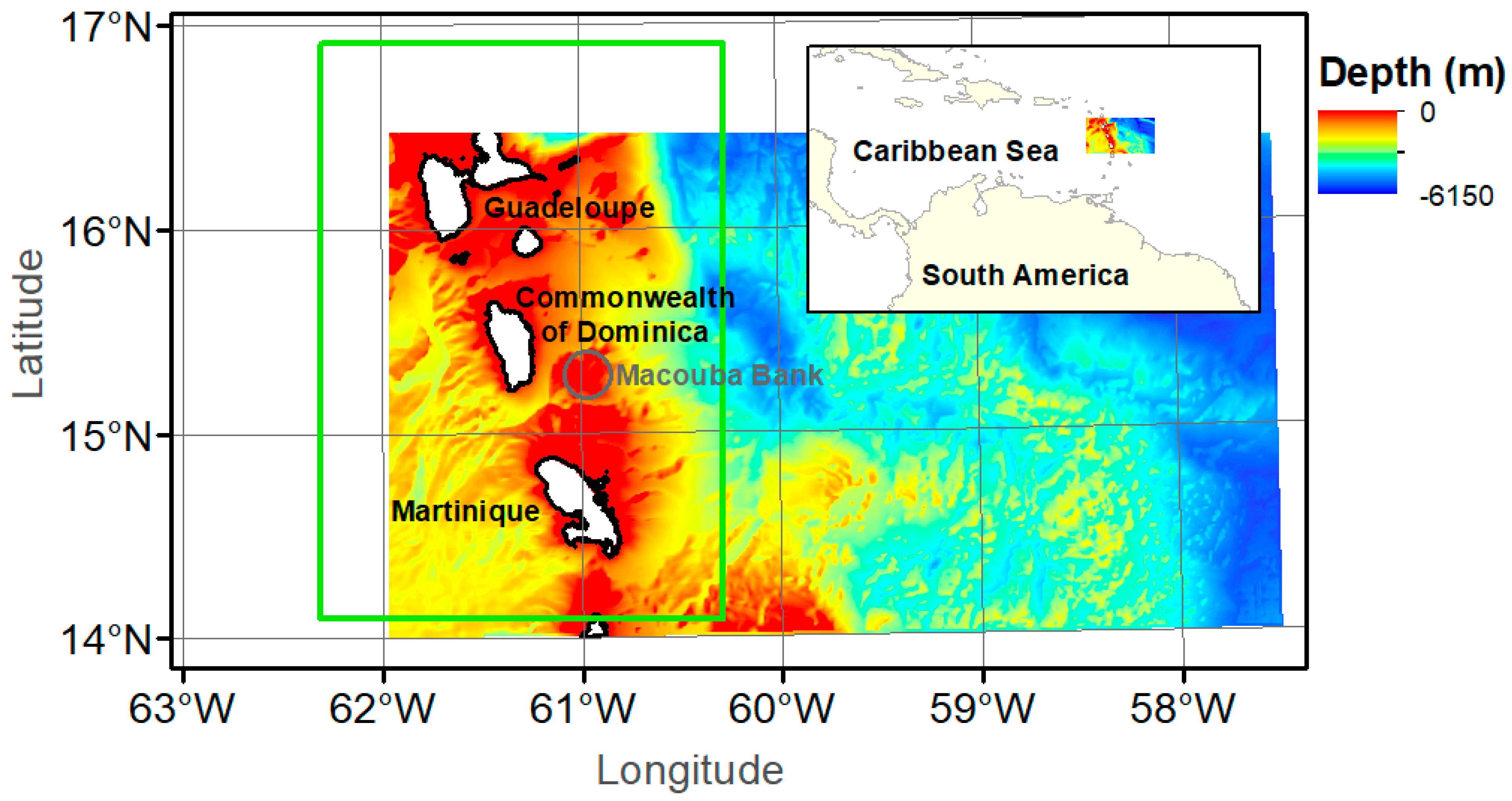
2.1. Study Area

The study area consists of the Commonwealth of Dominica and surrounding waters, first using a large bounding box extending from 57.5°W to 63°W (~586 km) and 14°N to 16.9°N (~320 km). This covers an area of ~188,000 km² including several Caribbean Islands and stretches into the abyssal plain of the NW Atlantic (Figure 1). Second, a smaller bounding box is used, extending from 60.3°W to 62.3°W (~215 km) and 14°N to 16.9°N (~320 km), covering an area of ~68,800 km². This smaller area study was conducted to focus on the shallower marine environment surrounding the Caribbean Islands, without extending further into the NW Atlantic or Caribbean Sea. Removing the influence of the deeper, further offshore region may reveal patterns in the nearshore clusters that give us greater insight into these shallower waters, but it has the risk to ignore wider environmental patterns.

2.2. Data

2.2.1. Bathymetric Data

Two sources of bathymetric data were used within this study. The first data source, at 800 m resolution, is the General Bathymetric Chart of the Oceans (GEBCO) [31] and the boundaries of this dataset (57.5°–63.0°W and 14.0°–17.0°N) were selected to include the entire Dominican Exclusive Economic Zone (EEZ), which extends from 57.875° to 62.8139°W and 14.4886° to 16.5008°N [32]. The second bathymetry dataset is a digital elevation model (DEM) of Guadeloupe and Martinique produced as part of the HOMONIM (History, Observation and Modelling of sea levels) project [33]; piloted by the French Naval Hydrographic and Oceanographic Service (SHOM) and the French national meteorological service (Météo-France).

This DEM encompasses several of the Lesser Antilles Islands, from Montserrat in the north to Saint Lucia in the south and extends offshore to a depth of 5800 m. It is comprised of SHOM bathymetry combined with existing compilations of DEM (GEBCO, EMODnet etc.) and bathymetric data from international databases. The boundaries of the smaller dataset defined the extent of the local scale study, extending from 60.3° to 62.3°W and 14.0° to 17.0°N. This dataset had a resolution of 100 m, but due to noise in the data, a Gaussian Filter (Standard deviation 20, radius 40) was applied in SAGA GIS (version 7.2) to soften noise that might affect the clustering process (see landscape mapping).

Both datasets were interpolated to 250 m resolution and then combined using the TOPOGRID interpolation function in ArcGIS (version 10.6). This function uses the ANUDEM algorithm, a computationally efficient multigrid interpolation process, which aims to account for errors in large datasets without over-smoothing well-defined features [18,34,35]. The SHOM dataset was prioritised due to its initial higher resolution and a 1000 m surrounding buffer with no data were applied to smooth the boundary joining.

Following the creation of an initial map, which demonstrated clusters in unnatural straight lines, highlighting the survey artefacts in the data, the mean Focal Statistics function in the Spatial Analyst toolbox of ArcMap was used (a neighbourhood settings of three cells) to further reduce the noise associated with the bathymetric data. This process created a smoother DEM with output cell values that are a function of the original cell values in a specified neighbourhood around the focal cell.

From this combined grid, the following bathymetric derivatives were calculated (summarised in

Table 1. Bathymetric derived variables included in the landscape mapping analysis.

Bathymetric Derivatives	Description	Calculated
Slope	Gradient of bathymetry	Slope Spatial Analyst Tool in ArcMap (using a 3 × 3 cell neighbourhood)
Topographic Position Index	Compares elevation of focal cell to all cells in a specified neighbourhood	Land Facet Corridor Tools extension in ArcMap, radius of 4 cells (1000 m)
Terrain Ruggedness Index	The mean difference between a focal cell and the surrounding cells in a specified neighbourhood	SAGA GIS Terrain Analysis Morphometry, radius of 4 cells (1000 m)
Plan Curvature	Curvature of the surface perpendicular to the slope direction	Curvature Spatial Analyst Tool in ArcMap (using a 3 × 3 cell neighbourhood)

): within ArcMap slope and plan curvature were derived using the Spatial Analyst Toolbox (using a 3 × 3 cell neighbourhood). Topographic position index (TPI) was calculated using the Land Facet Corridor Tools extension in ArcMap (radius of 4 cells, 1000 m). Terrain ruggedness index (TRI) was calculated using the SAGA GIS Terrain Analysis Morphometry tools (radius of four cells, 1000 m).

Multiple scales of the same variables were highly correlated and so, rather than including them all, finer scale plan curvature and slope were used to capture finer patterns (gullies and canyons) while broad scale TPI and TRI were used to capture broad patterns. Plan curvature was selected, as it is the least correlated with TPI.

2.2.2. Satellite and Oceanographic Model Derived Variables

Seabed salinity, temperature and current velocity data were derived from the Copernicus Global Sea Physical Analysis and Forecasting numerical model [36] at a spatial resolution of 0.083 degrees × 0.083 degrees (~8900 m by longitude and ~9100 m by latitude at the latitude of study). Contrary to Hogg et al. [18], who split oceanographic variables into summer and winter averages, we used annual mean values, given the limited annual variation in water column characteristics at this latitude. Satellite derived net primary productivity (NPP) data were sourced from Oregon State University [37] (http://sites.science.oregonstate.edu/ocean.productivity, accessed 8 March 2019), as monthly means at 1/12 degree spatial resolution. NPP is defined as a function of the Vertically Generalised Production Model, MODIS surface chlorophyll concentrations, MODIS 4-micron sea surface temperature and MODIS cloud-corrected incident daily photosynthetically active radiation (PAR).

Table 2. Satellite and Oceanographic Model derived variables included in the landscape mapping analysis.

Satellite and Oceanographic Model Variables	Source	Calculated
Net Primary Production (mg C/m2/day)	Oregon State University Vertically Generalised Production Model	Monthly data averaged over 3 years (January 2016–December 2018)
Salinity (PSU)	Copernicus Global Ocean Model Timeseries
Temperature (°C)
Current (m/s)

provides a summary of satellite and oceanographic model derived variables included in the landscape mapping analysis. These data were imported into RStudio (version 2021.9.1.372) where they were filtered to the region of interest and an average of the monthly means from January 2016 to December 2018 was calculated.

These data were then imported into ArcMap, transformed to WGS 84 UTM 20N and interpolated to a spatial resolution of 250 m using the Spline with Barriers function from the Spatial Analyst Toolbox. The island’s coastline was used as the barrier to prevent interpolation across the terrestrial landscape.

2.3. Landscape Mapping

This study follows the method adapted by Hogg et al. [18], to create a landscape map of sub-Antarctic South Georgia, following Verfaillie et al. [17] and Ismail et al. [19]. The following analysis was conducted in RStudio [38] (package ‘psych’ [39]), with the data normalised to have zero-means and unit variance. The stages were as follows:

• Principal component analysis (PCA). PCA was conducted on the nine input variables to reduce the data to linearly independent Principal Components (PCs) and remove collinearity. These PCs account for the greatest variance in the data without needing to predetermine which variables should be used for the analysis. PCs with eigenvalues less than 1 are traditionally discarded following the Kaiser-Guttman criterion; however, the initial eigenvalues calculated from the larger dataset had one borderline value and so the study was performed using both values >1 and >0.97. A Varimax rotation of the retained PCs was performed, to clarify the loadings matrix structure, and the subsequent analysis was performed on the resulting rotated PCs (RPCs).
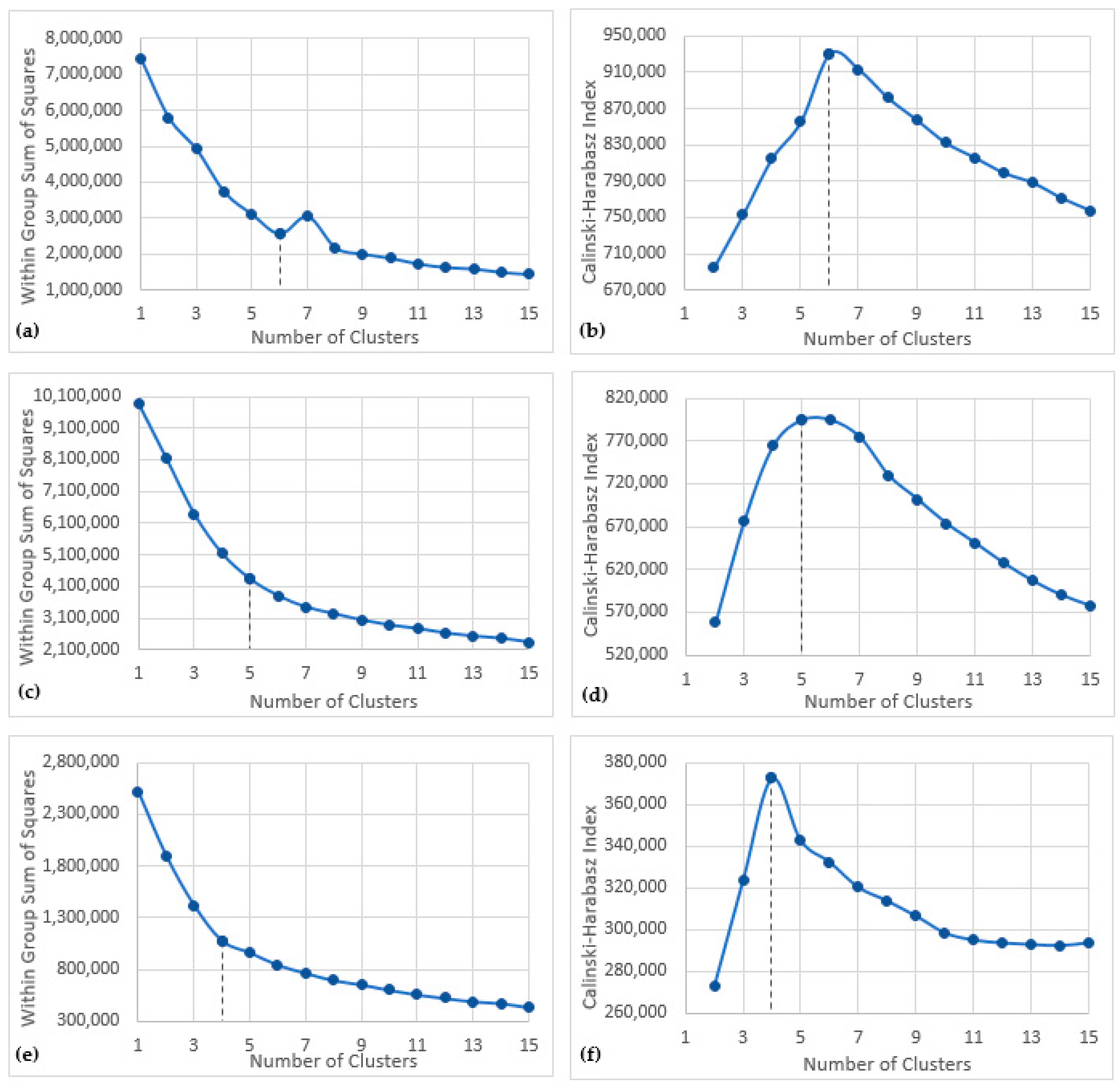
• Determine optimum number of clusters. A predefined number of clusters must be input into the K-means clustering algorithm. Here we used both the Calinski-Harabasz index (C-H) [40] and the elbow method [22] to determine the number of clusters. The C-H index is the ratio of the sum of inter-cluster variance to the intra-cluster variance; the highest value indicates the optimum number of clusters. The elbow method assesses the variance within clusters against a range of cluster values (here 1–15). The point at which increasing the number of clusters does not significantly lower the intra-cluster variance is the optimum number of clusters.
• K-means clustering. K-means clustering is a common algorithm used to partition marine environmental data [17,41]. The number of clusters for K-means clustering must be specified for this analysis; both the Calinski-Harabasz index (C-H) [40] and the elbow method [22] will be used to determine this value in an objective way. The K-means clustering algorithm uses an iterative method, whereby cluster centres are randomly allocated, and each data point is temporarily assigned to the cluster that minimises the distance between the focal point and the centre of the cluster in the multidimensional PC space. The centre points are then repeatedly shifted, the distances recalculated, and the data points re-allocated to the closest cluster centres, until the positions of the centroids are optimal or until the specified number of iterations has been reached.
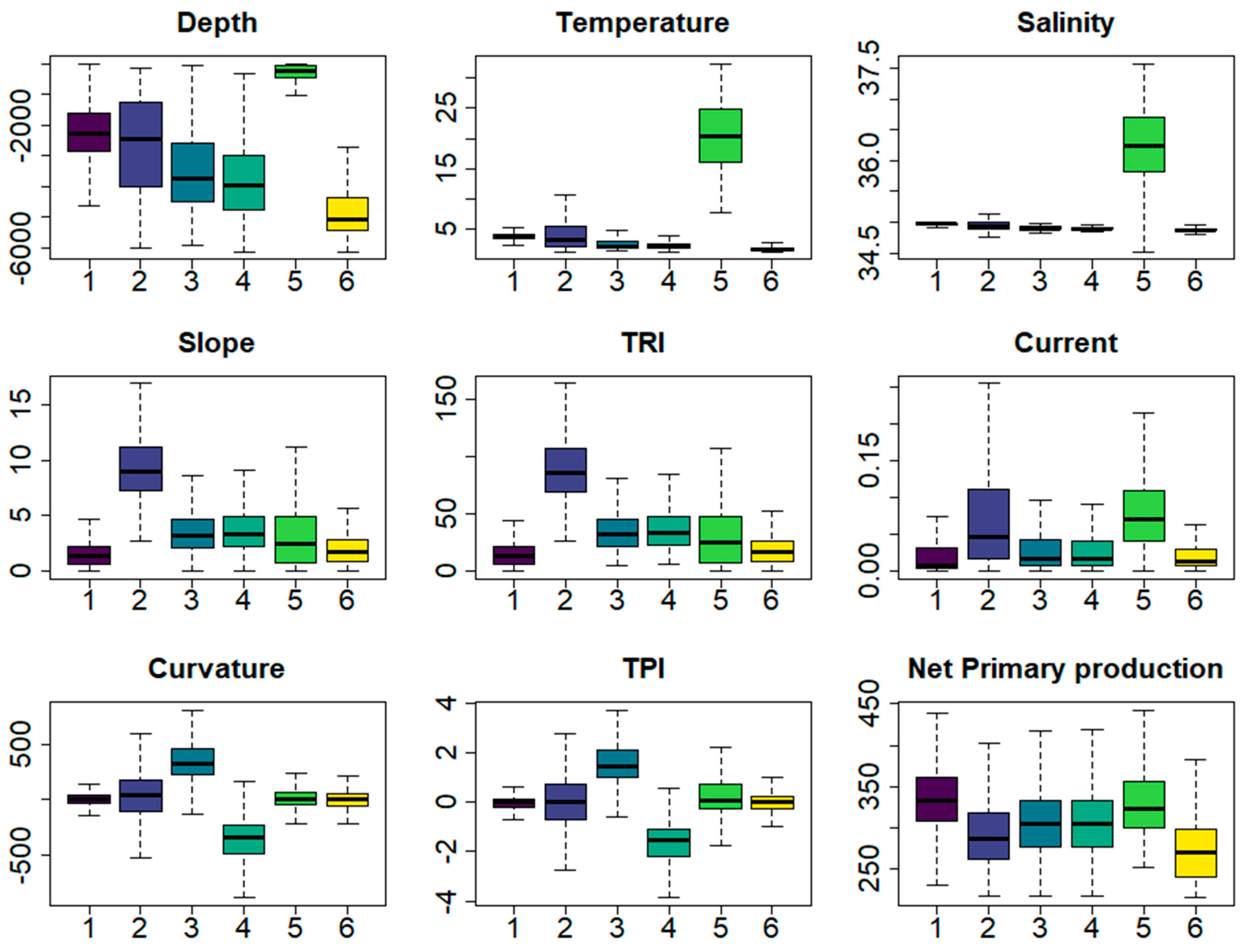
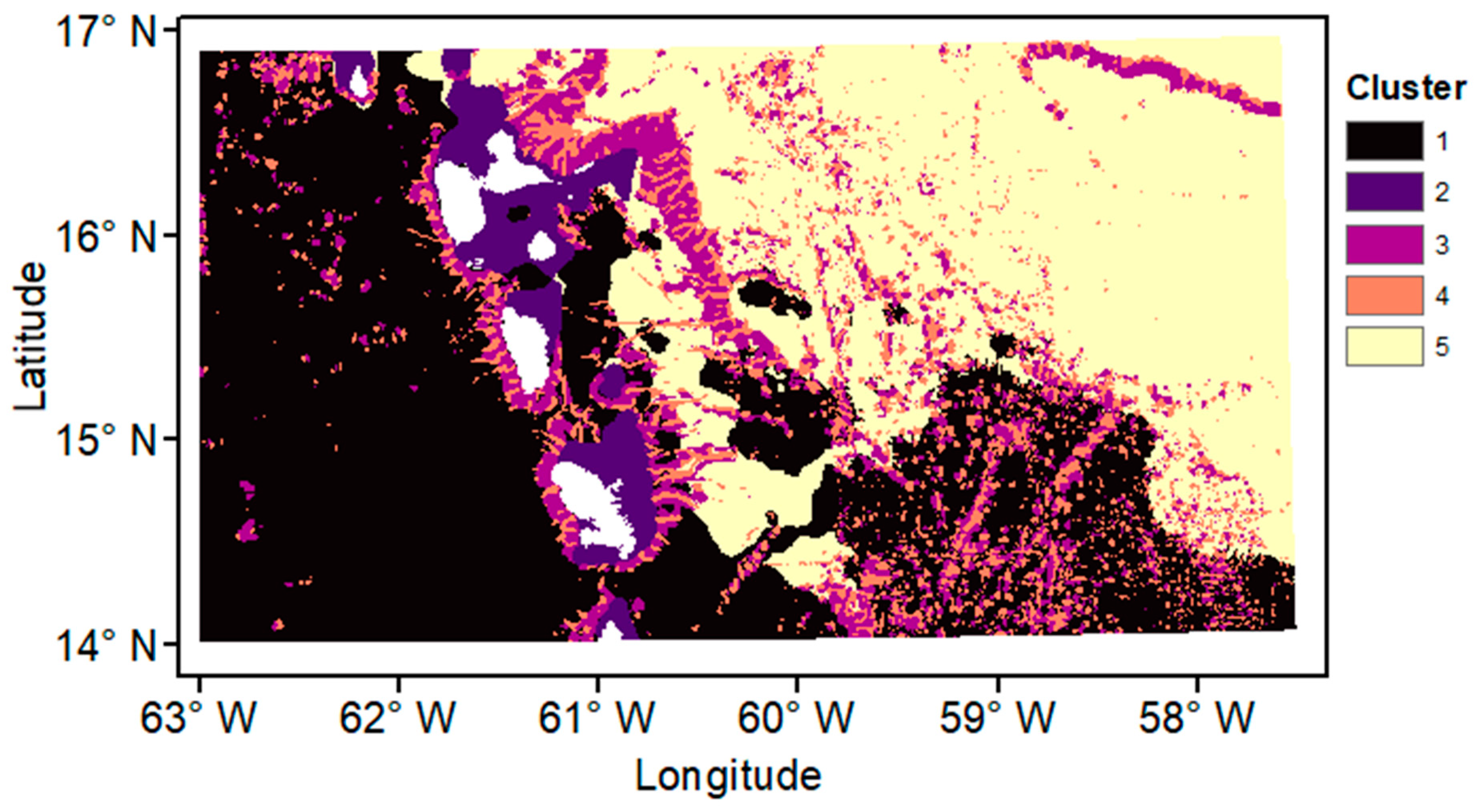
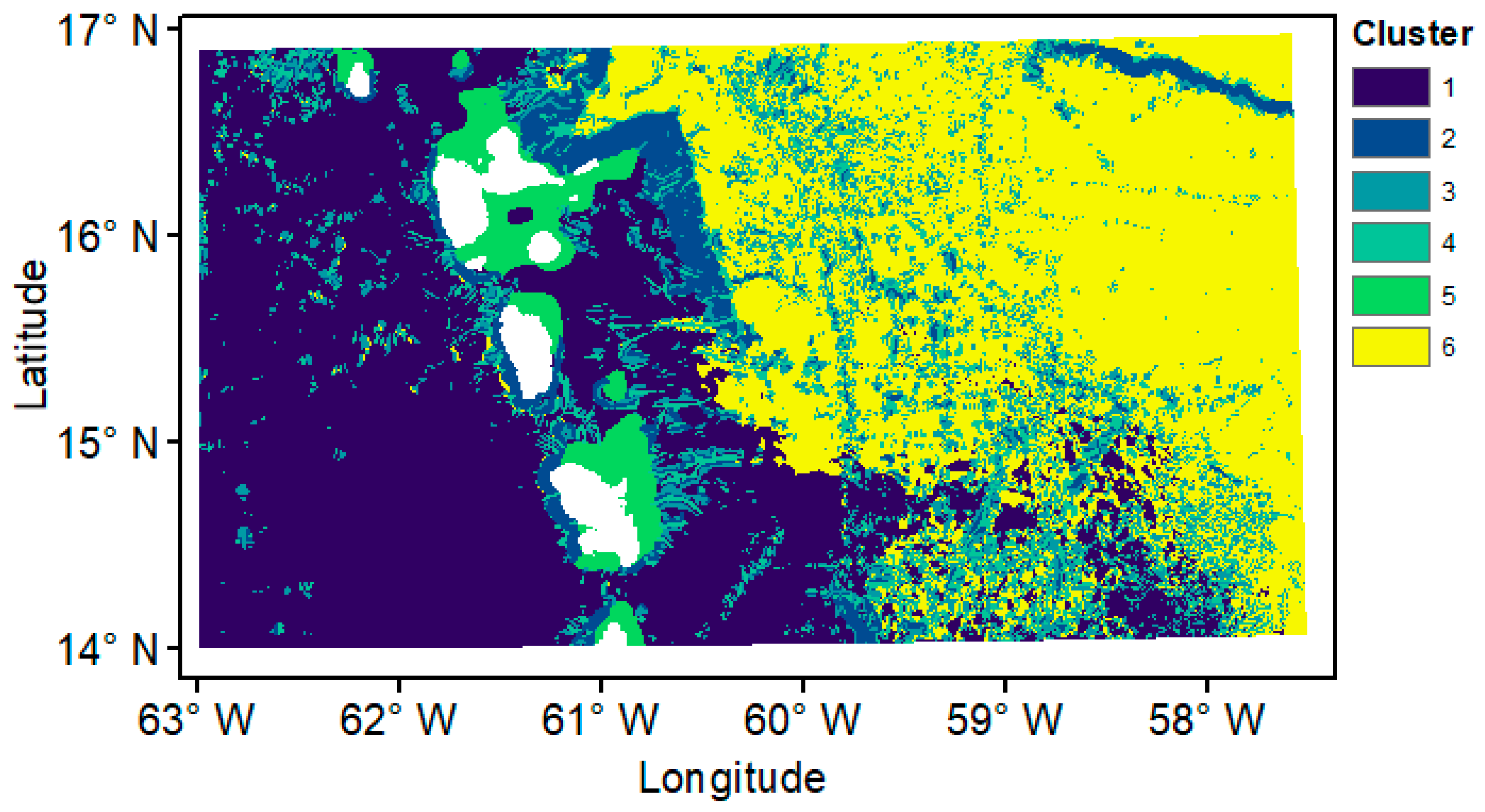
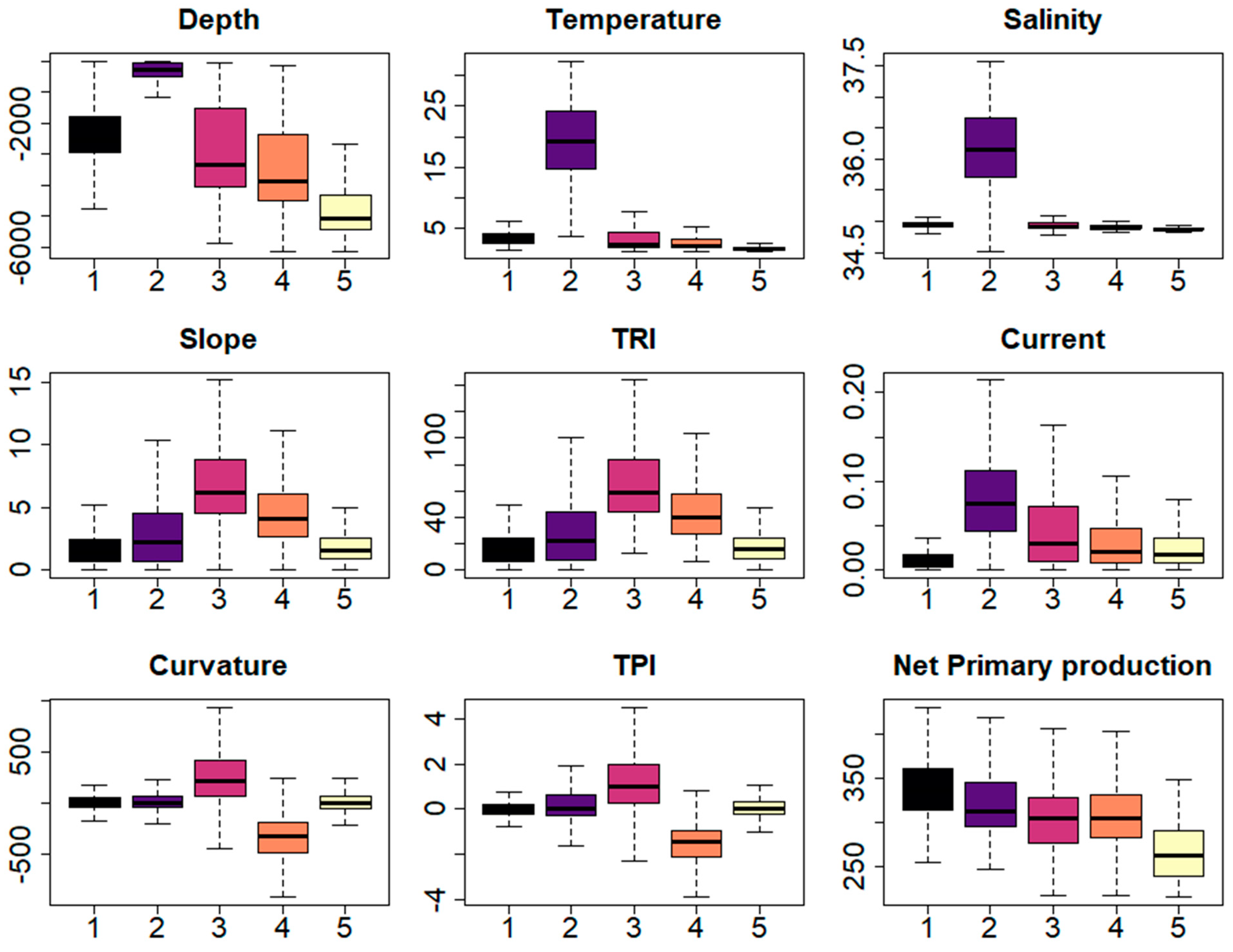
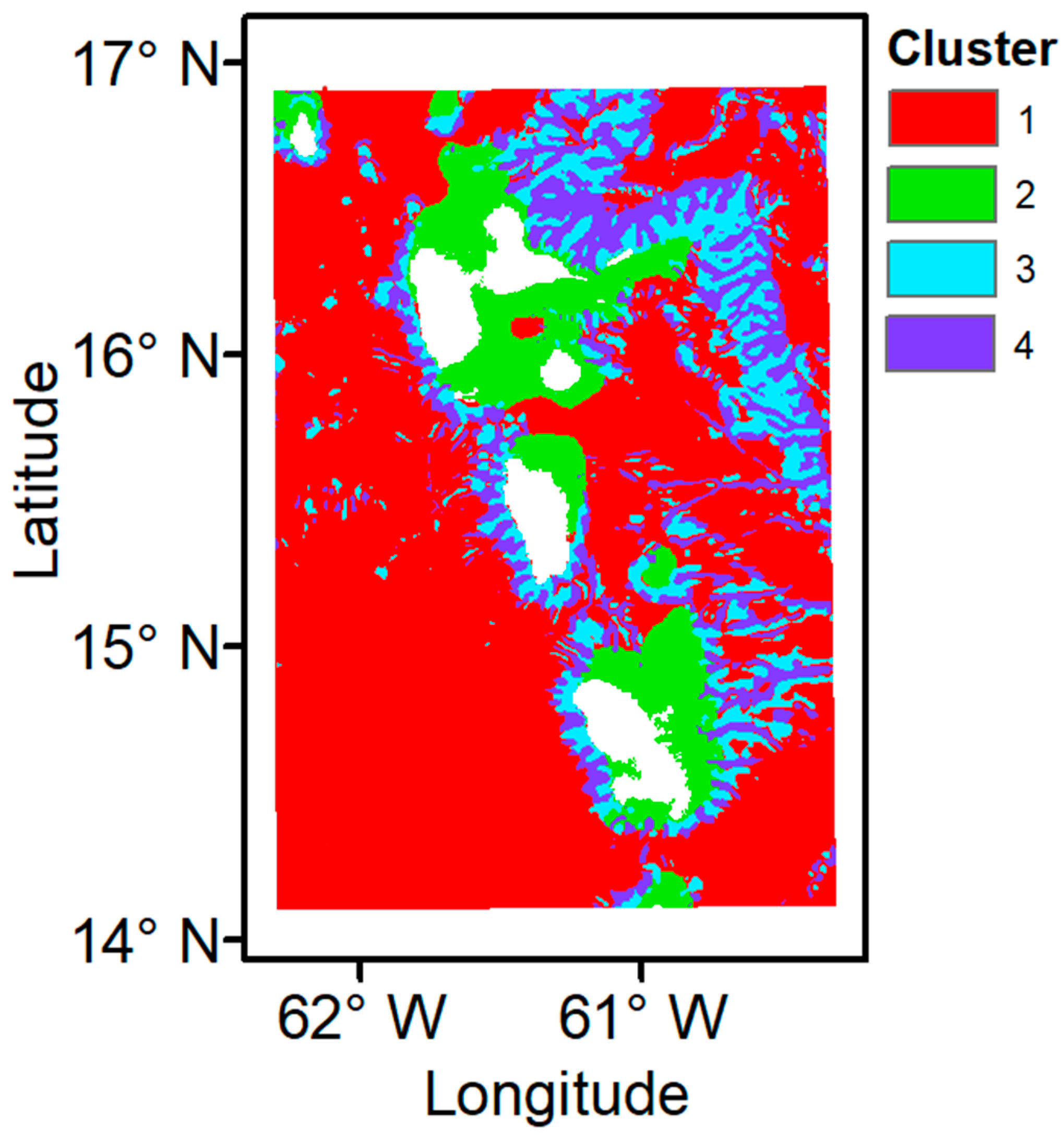
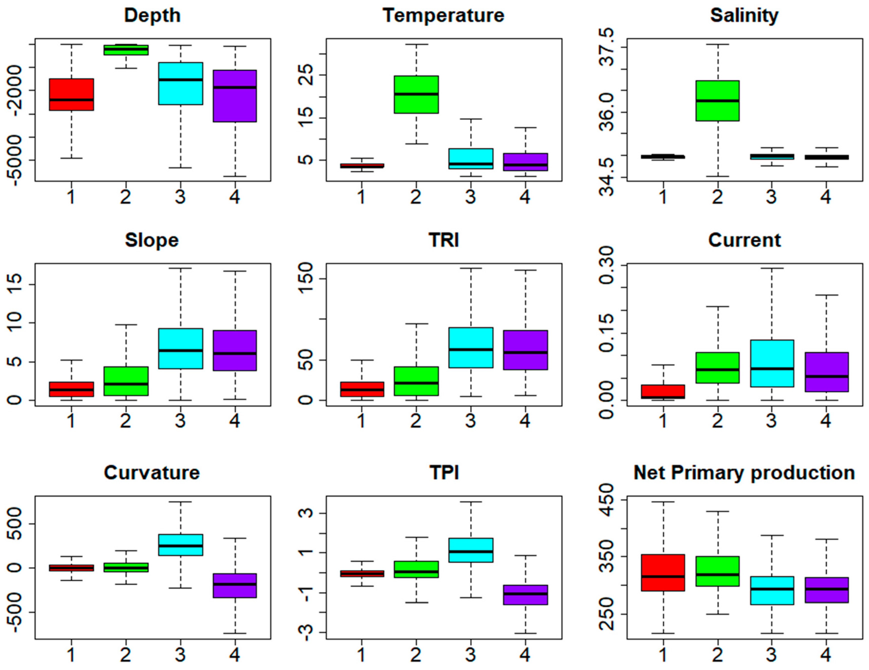
• Landscape map. The final cluster value for each data point was plotted against the point location to create a landscape map of the study regions. Boxplots summarising the distribution of the original input abiotic variables against the K-means cluster values were created to assess the influence of the abiotic inputs on the cluster solution and determine the physical characteristics of each cluster.
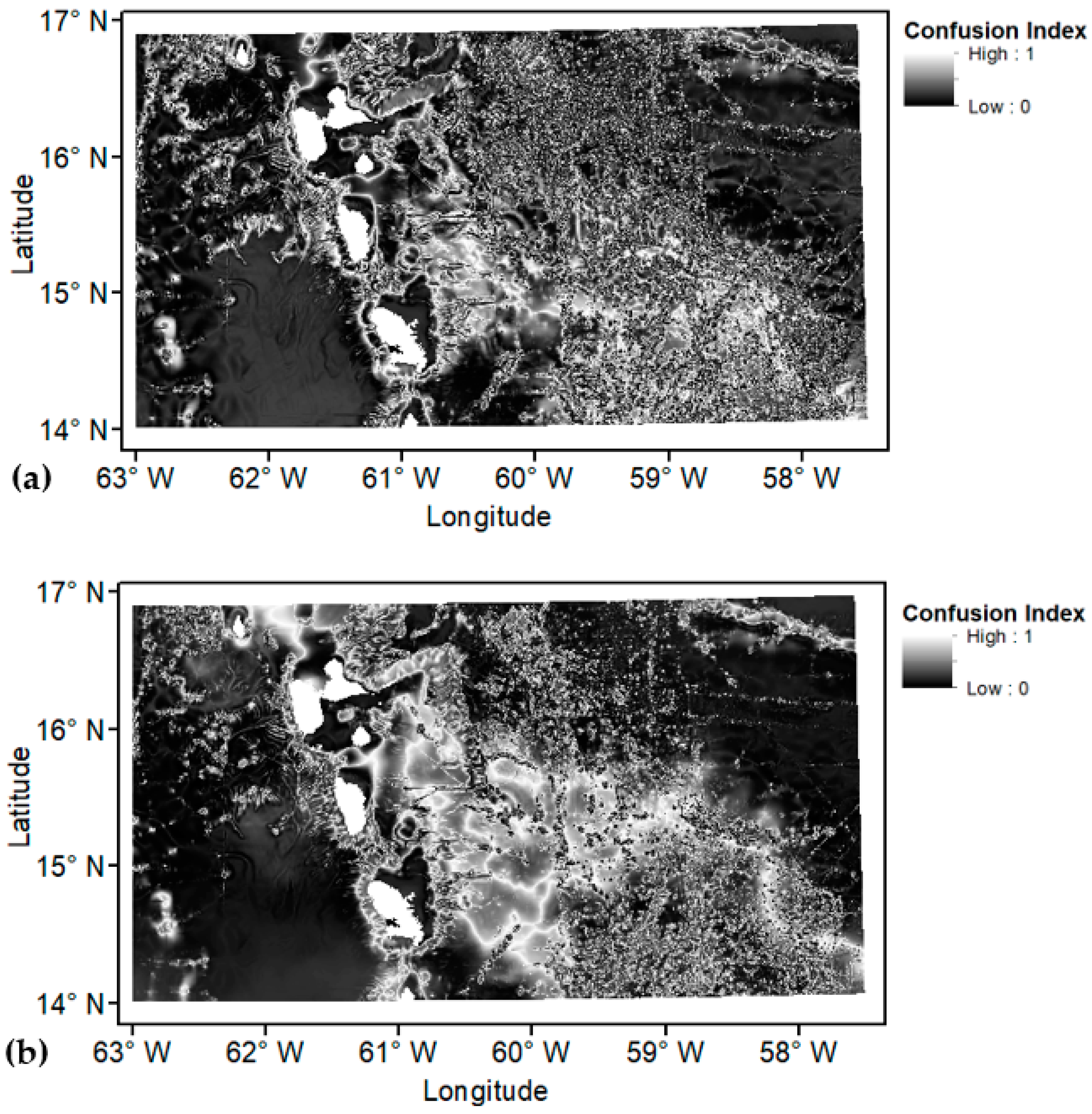
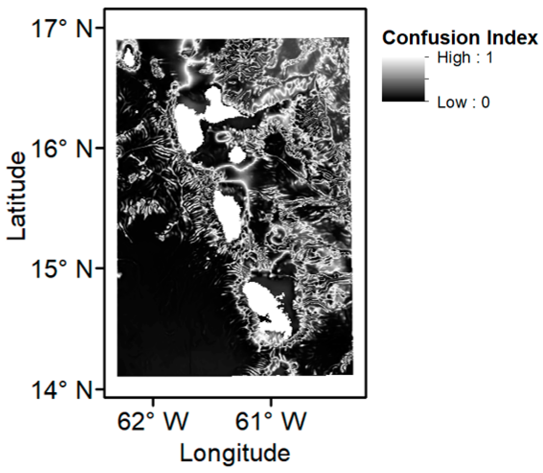
• Confusion Index Map. To assess how well each data point fitted within its assigned cluster, a confusion index map was created using the inverse distance squared in attribute space between the data observation and each K-means cluster centre to give a cluster membership value. A quantitative uncertainty measurement can be calculated using, for each data point, the ratio of the second highest membership value versus the highest, known as a confusion index (CI) [19]. If the data point is well characterised by the assigned cluster, the CI value will approach zero. Conversely, if the data point is not dominated by the assigned cluster, and the membership values are spread across several clusters, the value will be closer to one. These values were plotted against the data observation location to create a confusion map. For more detail, see Hogg et al. [18].

3. Results

3.1. PCA and Eigenvalues

3.1.1. Larger Study Area

Principal component analysis (PCA) performed on the larger study area variables resulted in three eigenvalues greater than one, and one eigenvalue of 0.980 (

Table 3. Eigenvalues for the larger study area.

Larger Study Area	PC1	PC2	PC3	PC4	PC5	PC6	PC7	PC8	PC9
Standard deviation	1.684	1.411	1.330	0.990	0.862	0.611	0.468	0.294	0.057
Proportion of Variance (%)	31.500	22.122	19.643	10.894	8.263	4.148	2.436	0.958	0.036
Cumulative Proportion (%)	31.500	53.622	73.265	84.159	92.422	96.570	99.006	99.964	100.000
Eigenvalue	2.835	1.991	1.768	0.980	0.744	0.373	0.219	0.086	0.003

). To assess the significance of including this fourth principal component (PC), two landscape maps were created; henceforth these two maps shall be referred to as E3 (three eigenvalues used) and E4 (four eigenvalues used). Taking only the initial three PCs with eigenvalues of one or greater, 73.265% of the total variance was explained, while the addition of the fourth RPC with eigenvalue 0.980 explains a further 10.894% of the variance.

Varimax rotated principle component analysis (RPCA) performed on the E3 data (

Table 4. Rotated components matrix. Correlation between the original input variables and the Varimax rotated principal components for the larger study area using three eigenvalues. Values with r > 0.7 or r < −0.7, are considered high factor loads (bold), while low factor loads (r < 0.3 or r > −0.3) are omitted.

Abiotic Variables (E3, Large)	RPC 1	RPC 2	RPC 3
Depth	0.829	-	-
Slope	-	0.974	-
Plan Curvature	-	-	0.943
Topographic Position Index	-	-	0.942
Terrain Ruggedness Index	-	0.975	-
Salinity	0.837	-	-
Current	0.352	0.441	-
Temperature	0.908	-	-
Net Primary Productivity	0.532	-	-

), resulted in RPC 1 having high loads for depth, salinity, and temperature and lower loads for NPP and current; RPC 2 had high loads for slope and TRI and a lower load for current; RPC 3 had high loads for plan curvature and TPI. Joint high loadings on one RPC clearly illustrate correlation between those variables.

In the E4 RPCA (

Table 5. Rotated components matrix. Correlation between the original input variables and the Varimax rotated principal components for the larger study area using four eigenvalues. Values with r > 0.7 or r < −0.7, are considered high factor loads (bold), while low factor loads (r < 0.3 or r > −0.3) are omitted.

Abiotic Variables (E4, Large)	RPC 1	RPC 2	RPC 3	RPC 4
Depth	0.592	-	-	0.642
Slope	-	0.989	-	-
Plan Curvature	-	-	0.944	-
Topographic Position Index	-	-	0.942	-
Terrain Ruggedness Index	-	0.989	-	-
Salinity	0.908	-	-	-
Current	0.556	0.315	-	-
Temperature	0.909	-	-	-
Net Primary Productivity	0.055	-	-	0.928

), all abiotic variables had a connection with only one RPC, except for depth and current. RPC 1 had high loads for depth, salinity, and temperature as well as lower loads for NPP and current; RPC 2 had high loads for slope and TRI and a lower load for current; RPC 3 had high loads for plan curvature and TPI; RPC 4 had a high load for NPP and a lower load for depth.

3.1.2. Smaller Study Area

PCA performed on the smaller study area resulted in three RPCs with an eigenvalue of one or greater (

Table 6. Eigenvalues for the smaller study area.

Smaller Study Area	PC 1	PC 2	PC 3	PC 4	PC 5	PC 6	PC 7	PC 8	PC 9
Standard deviation	1.661	1.471	1.300	0.936	0.818	0.714	0.487	0.306	0.031
Proportion of Variance (%)	30.642	24.058	18.790	9.737	7.431	5.657	2.637	1.037	0.011
Cumulative Proportion (%)	30.642	54.700	73.490	83.228	90.659	96.315	98.952	99.989	100.000
Eigenvalue	2.758	2.165	1.691	0.876	0.669	0.509	0.237	0.093	0.001

), which explained 73.490% of the total variance and RPCA was performed on these PCs. The rotated components matrix (

Table 7. Rotated components matrix. Correlation between the original input variables and the Varimax rotated principal components for the smaller study area. Values with r > 0.7 or r < −0.7, are considered high factor loads (bold), while low factor loads (r < 0.3 or r > −0.3) are omitted.

Abiotic Variables (E3, Small)	RPC 1	RPC 2	RPC 3
Depth	0.798	-	-
Slope	-	0.948	-
Plan Curvature	-	-	0.937
Topographic Position Index	-	-	0.931
Terrain Ruggedness Index	-	0.948	-
Salinity	0.893	-	-
Current	0.338	0.535	-
Temperature	0.951	-	-
Net Primary Productivity	-	−0.490	-

) shows the factor loads which explain the correlation between the RPCs and the original abiotic variables, excluding any factor loads −0.3 > r < 0.3. All variables had a high factor load (r > 0.7) with only one RPC, except current and NPP. RPC 1 had a high load for the variables depth, salinity, and temperature; RPC 2 for slope and TRI; RPC 3 for plan curvature and TPI. NPP had a lower factor load with RPC 2 and current had a lower factor load with RPCs 1 and 2.

3.2. Clustering and K-Means

3.2.1. Larger Study Area

For the larger study area, the ‘elbow method’ was applied to the within group sum of squares clustering solution. The gradient change in the graph, which would identify the optimal clustering solution, was unclear for both the E3 and E4 studies (Figure 2a,c, respectively). The Calinski-Harabasz method showed clear first local maxima for both the E3—six clusters (Figure 2b) and E4—five clusters (Figure 2d) studies, and so these values were used for the following K-means analyses.

3.2.2. Smaller Study Area

The result of the group sum of squares clustering solution for the smaller study area was evident at four clusters (Figure 2e). The Calinski-Harabasz method agreed, showing a clear first local maximum at four clusters (Figure 2f) and so this value was used for the following K-means clustering.

3.3. Broadscale Landscape Map

The results of the K-means analysis clustering solution were interpreted alongside the boxplots of the distribution of the original input variables for each cluster.

3.3.1. Larger Study Area

The E3 area resulted in six clusters (Figure 3), each of which had distinct physical conditions (Figure 4). Clusters 1 and 6 occur in deeper waters and were influenced by the eastward transition from high to low NPP. Cluster 2 occurs in areas of steep slopes and high TRI, as well as higher currents and a broad range of plan curvature and TPI, indicating an area of depressions and peaks. This cluster occurs on the west side of each island, on the shoulder to the northeast of Guadeloupe and along a ridge to the northeast of the study area. Clusters 3 and 4 were characterised by plan curvature and TPI, occurring on the sides of slopes and around the islands where the seafloor drops into deep water. Cluster 3 occurs in high TPI and curvature indicating peaks and ridges and cluster 4 in low TPI and curvature indicating gullies or canyons. Cluster 5 occurred predominantly to the east of each island in shallow depths, high temperatures and high salinity waters with a broad range of currents. Small features occur throughout the study area to the east of the islands.

The E4 study area demonstrates similar cluster characteristics to the E3 map; however, the four eigenvalues resulted in only five clusters (Figure 5 and Figure 6). Clusters 1 and 5 demonstrate the declining NPP gradient from east to west. Cluster 2 is defined by shallow, high temperature and high salinity waters. However, clusters 3 and 4 represent the areas covered by the E3 clusters 2, 3 and 4 and are characterised by slope, TRI, plan curvature and TPI.

3.3.2. Smaller Study Area

The smaller study area was clustered into four regions (Figure 7) and was characterised in a similar manner to both the larger studies (Figure 8). Cluster 2 was characterised by shallow, high temperature, high salinity water to the east of the islands while clusters 3 and 4 represented the areas of high slope and ruggedness (TRI), and range in plan curvature and TPI. Cluster 1 represented the remaining deeper water but did not demonstrate the gradient in NPP shown in the larger area. In this local map, the shoulder to the east of Guadeloupe is divided into two clusters, similar to the E4 map, demonstrating that the difference in plan curvature and TPI is more significant than depth and slope.

3.4. Confusion Index Map

3.4.1. Larger Study Area

Figure 9 shows the confusion index maps for both E3 and E4, with the confusion index for each study scaled between 0 and 1. Around the islands, the confusion index map is dark, showing low confusion in the assigned cluster for each study and indicating the regions dictated by depth, salinity and temperature are distinct. The area to the southwest of the islands also demonstrates low confusion, although the E4 study is darker in this region than the E3 study, indicating the E3 study has higher confusion in the assigned cluster for that region. The same occurs in the northeast of the map extent.

The shoulder to the northeast of Guadeloupe is more distinctly dark in the E3 study, where the shoulder was classed as one cluster, whereas in the E4 study, where the shoulder was divided into two clusters, the region has higher confusion. The highest confusion occurs at the boundaries of the clusters, as the characteristics of the region transition between defining variables. High confusion is indicative that the habitats have characteristics of more than one cluster. The E3 patchiness of the smaller features to the east of the islands is more apparent than in the E4 map but the western extent of cluster 5 in the E4 study has higher confusion than the E3 assigned clusters, particularly to the northeast of the Commonwealth of Dominica as cluster 5 transitions to cluster 1 along the NPP gradient.

3.4.2. Smaller Study Area

The confusion index map for the smaller study area (Figure 10) has extensive areas of low confusion to the southwest of the map extent, similar to the larger study areas. Most of the higher confusion zones appear at the cluster boundaries. Areas of lighter grey occur to the northeast where cluster 1 reaches around the islands, in the region the broadscale maps transition to another cluster due to the NPP gradient.

4. Discussion

4.1. The Marine Landscape around Dominica

Each of the studies above maps environmental zones based on abiotic factors derived from publicly available data. This demonstrates the potential of open access data, and, while the method does not determine where ecologically important habitats are located, it highlights areas of potential interest without the input of biological data. The results can be used to identify areas of survey priority and in need of MSP, be a starting point for stakeholder discussion, and be incorporated into MSP development and MPA designation through defining and analysing existing conditions and highlighting potential areas of interest. If conservation efforts need to be focused on just one or a few areas, selecting the areas of highest habitat heterogeneity—the areas with the highest number of clusters, and therefore habitats, within close proximity—can allow each habitat to be included within the MSP. Additionally, calculating the area covered by each cluster can contribute to proportional conservation target achievement. The marine landscape maps can be used as input to quantify the structure (composition and configuration) of the offshore environment, using metrics such as those used in landscape ecology (e.g., Swanborn et al. [42]). At the same time, it may be possible to apply some local knowledge of the nearshore environment to offshore areas that have been allocated to the same cluster.

Previous studies of the nearshore distribution of benthic habitats in Dominican waters revealed seagrass habitats dominate the west and north coast of the island, with coral reefs also occurring in these regions [13,43,44]. In the E3 study, this western nearshore region is classified predominately as cluster 2, with areas of clusters 3 and 4, the same as the shoulder to the northeast of Guadeloupe, the southern tail of which lies within Dominican waters, and is characterised by higher slope, TRI, and currents. In the E4 and smaller area study both areas are more evenly divided between clusters 3 and 4, characterised by slope, TRI, TPI and plan curvature, as these clusters in E4 account for clusters 2, 3 and 4 in E3. Hydrodynamics and terrain complexity strongly influence habitat suitability [45,46]. While this dataset lacked substrate type, which is also influential in determining habitat assemblages, the inclusion of bathymetric derivatives such as rugosity and slope can be an indicator of substrate type [47]. Areas of high slope and current are often indicative of hard substrate, due to low sedimentation or erosion. Higher current velocity and terrain complexity have also been linked with increased biodiversity [46]. A relationship between filter-feeding communities and increased (up to limiting values) slope, near-bottom currents and resultant turbidity has been demonstrated, as these organisms feed on particles suspended in the water [45,48]. Habitats identified from previous nearshore studies of areas that lie in the same cluster as the southern tail of the shoulder can be used to infer whether further investigation of this area is warranted.

Rocky and sandy areas comprise 81% of the shallow marine benthos of Dominica and dominate the south and east coast [13] where the topography is not as steep as the west. The shelf area, characterised by shallow, higher temperature and salinity waters is comparatively much smaller for Dominica than the surrounding islands. Each of the broadscale landscape maps identify a bank to the southeast of Dominica that demonstrates the same characteristics, defined by shallow depth, higher temperature, and salinity, as the nearshore waters on the northeast of the islands. This is Macouba bank, partially within Dominican waters but, as it is ~24 km from the coast, it is difficult for the smaller Dominican fishing boats to access and has allegedly been exploited by fishers coming from other nations with more established fishing gear [49,50]. If this is an area of ecological and environmental interest, as it has waters of similar characteristics to the more productive shallow Dominican waters, it might be a priority for future management and investigation. It is also of note that the more productive shallow waters on the Dominican coast lie to the northeast of this island and fishers from this area would have to travel over 40 km to reach the exposed waters of Macouba Bank. This distance could also present difficulties with management and policing of this bank.

4.2. Unsupervised Classification: Methodological Considerations

The purpose of PCA is to reduce the dimensionality of the input data and to ensure the input variables are independent. A significant consideration for this study was how many PCs to include within the analysis. An eigenvalue >1 explains more variance in the data than the individual input variables. Therefore, the initial study follows this rule. However, as computers have developed, constraining the dimensionality of the data is less important and the priority is reducing the correlation between variables. Therefore, the E4 study was also conducted to prevent loss of variability in the dataset. By including the fourth eigenvalue, a further 10.894% of the variance was included in the map. This additional data may be a deciding factor in the cluster assignment of a data point where the confusion index is high.

The difference between the E3 and E4 study is the amalgamation of E3 clusters 2, 3 and 4 into E4 clusters 3 and 4, removing the separation between the TRI/slope and curvature/TPI characterised clusters. This is most apparent in the shoulder to the northeast of Guadeloupe, and while the confusion index for the E3 study is low in this area, the boundaries of the shoulder clusters in the E4 study have higher confusion. This indicates that depth, salinity, temperature and NPP have a stronger influence on the segmentation of this dataset than the other variables.

By including the fourth eigenvalue in the E4 study and losing the sixth cluster, it could be said that too much variance is included and this has diluted the contribution of the other eigenvalues and increased the map confusion. The E3 study shows more detail, by including the sixth cluster and separating the TRI/slope and curvature/TPI contributions, it also has lower confusion in the region to the east of the islands. It is of note that in the smaller study area the shoulder to the northeast of Guadeloupe is divided into two clusters, similar to the E4 study. The influence of the NPP gradient is not seen in the smaller study, indicating that the TRI/slope and curvature/TPI variables are more significant in this smaller area. The smaller extent study was conducted to focus on the abiotic characteristics impacting the nearshore waters; however, as the clustering in this region seems to repeat in the larger extent studies, removing the deeper, offshore water influence has been shown to not greatly influence the clustering result, and no further patterns were revealed in the shallow waters. By conducting the larger extent studies, the NPP gradient influence has been highlighted, providing context information for the Dominican marine environment.

While this approach is unsupervised and objective in its clustering of the environmental variables, careful consideration of the input variables had to be conducted. Equal weighting is given to each variable; therefore, if there is an imbalance of topographic versus oceanographic variables, the results may be skewed towards the dominant data input. To improve upon this, a review of initial results was used to infer the importance of the input variables and consider their inclusion throughout the study. Furthermore, normalising the data to make the range of values in all variables comparable also means that even if there is very little change in a variable, these values will be stretched to make them as significant as the other data, which may have significant impacts on the final map. The assumption that organisms are equally influenced by each variable is inherent in this equal weighting approach. It is a valid default starting position if very little is known about the area or its fauna. Subsequent investigations should clarify if this assumption holds for the area under investigation.

Using bathymetric data sourced from multiple surveys, collected over a large area using different equipment and with varying resolution, and creating secondary derivatives from these merged surfaces, means any artefacts or errors included in the initial data will be propagated throughout the analysis and may bias results. As there was no access to raw data, which would have taken considerable time to process, it was necessary to use already processed bathymetry layers. The noise remaining from survey artefacts would have presented in the data as higher topographic complexity, e.g., higher rugosity or gradient. This was evident in the initial broadscale map and demonstrates how the results of the analysis are determined by the quality of the input data. The mean Focal Statistics function in the Spatial Analyst toolbox of ArcMap was used to reduce the noise in the bathymetric data, by creating a new value for each cell that is a function of the specified surrounding cells; however, by dampening the noise there is also loss of detail, and so a balance between detail and noise must be reached. Additionally, rather than grid at the coarsest resolution and lose the finer detail available, it is preferable to resample both the higher (100 m) and lower (800 m) resolution bathymetric surfaces to a middle ground (250 m). The low resolution of the open access bathymetric, satellite and oceanographic data means fine scale analysis is not possible. As data coverage and resolution increase in the future, and models advance, the resolution of the final products will also improve.

As part of our study, it was decided to include surface NPP values as a predictor of benthic characteristics. An implicit assumption in this approach is that benthic habitats are equally connected to surface productivity at all locations. The range of water depth in our study was 0–6200 m. However, the impact of primary production upon the benthic community will be influenced by the vertical attenuation due to remineralisation of the organic carbon as it sinks through the water column [51]. Therefore, at greater depths, the connection between surface and benthic environments may be reduced. Additionally, by assuming a one-dimensional water column, any lateral particulate organic carbon (POC) flux is neglected. Better POC estimates in deep waters at the benthic boundary layer would allow more accurate characterisation and the ability to distinguish between the range of benthic environments included in this study. The authors should discuss the results and how they can be interpreted from the perspective of previous studies and of the working hypotheses. The findings and their implications should be discussed in the broadest context possible. Future research directions may also be highlighted.

5. Conclusions

Based on publicly available datasets, we created broadscale landscape maps for the Commonwealth of Dominica and surrounding islands that allow us to assess the abiotic variables influencing the offshore benthic environment and to infer areas of interest for future study. Of particular note is Macouba Bank, an offshore area with similar characteristics to the productive nearshore environment of Dominica. It is proposed as a focus for future research and a priority for management. By defining and analysing existing conditions of the Dominican environment, the results of this study can be a starting point for MSP development.

The creation of the different extent maps highlighted the strong influence of NPP across the region and demonstrates that to capture large spatial patterns and context, sufficient spatial data coverage is needed.

The low resolution and high noise in the input data means fine scale analysis was not possible in this study; however, in areas of little available data, this method highlights the capabilities of publicly available datasets in providing context for a region. The equal weighting of the variables is both advantageous, as there is no prior knowledge of the most influential variables and so this method is objective, and disadvantageous, as with the equal weighting comes the assumption that all variables are equally influential on organism assemblages. However, careful consideration of the input variables and review of the initial results meant only variables considered important to the study were included in the final product. Our multiple clustering exercises also illustrated that inclusion of too many PCs in the K-means clustering could lead to an increase in the confusion index of the final output maps, and hence may not always be an advantage.

References

1. Halpern, B.; Walbridge, S.; Selkoe, K.; Kappel, C.; Micheli, F.; D’Agrosa, C.; Bruno, J.; Casey, K.; Ebert, C.; Fox, H.; et al. A Global Map of Human Impact on Marine Ecosystems. Science 2008, 319, 948–952. [Google Scholar] [CrossRef] [PubMed] [Green Version]
2. Diesing, M.; Green, S.L.; Stephens, D.; Lark, R.M.; Stewart, H.A.; Dove, D. Mapping seabed sediments: Comparison of manual, geostatistical, object-based image analysis and machine learning approaches. Cont. Shelf Res. 2014, 84, 107–119. [Google Scholar] [CrossRef] [Green Version]
3. Scobie, M. Global marine and ocean governance, and Caribbean SIDS. In Global Environmental Governance and Small States: Architectures and Agency in the Caribbean; Edward Elgar Publishing: Cheltenham, UK, 2019; pp. 90–117. [Google Scholar] [CrossRef]
4. Pinnegar, J.K.; Engelhard, G.H.; Norris, N.J.; Theophille, D.; Sebastien, R.D. Assessing vulnerability and adaptive capacity of the fisheries sector in Dominica: Long-term climate change and catastrophic hurricanes. ICES J. Mar. Sci. 2019, 76, 1353–1367. [Google Scholar] [CrossRef] [Green Version]
5. Fishery and Aquaculture Country Profiles: The Commonwealth of Dominica: The Commonwealth of Dominica. Available online: http://www.fao.org/fishery/facp/DMA/en (accessed on 8 January 2021).
6. Miller, K.A.; Thompson, K.F.; Johnston, P.; Santillo, D. An Overview of Seabed Mining Including the Current State of Development, Environmental Impacts, and Knowledge Gaps. Front. Mar. Sci. 2018, 4, 418. [Google Scholar] [CrossRef]
7. Cuyvers, L.; Berry, W.; Gjerde, K.; Thiele, T.; Wilhem, C. Deep Seabed Mining: A Rising Environmental Challenge; IUCN and Gallifrey Foundation: Gland, Switzerland, 2018. [Google Scholar]
8. Baker, E.K.; Harris, P.T. Habitat mapping and marine management. In Seafloor Geomorphology as Benthic Habitat, 2nd ed.; Harris, P.T., Baker, E., Eds.; Elsevier: Amsterdam, The Netherlands, 2020; Chapter 2; pp. 17–33. [Google Scholar] [CrossRef]
9. Cogan, C.B.; Todd, B.J.; Lawton, P.; Noji, T.T. The role of marine habitat mapping in ecosystem-based management. ICES J. Mar. Sci. 2009, 66, 2033–2042. [Google Scholar] [CrossRef]
10. United Nations Environment Programme. Emerging Issues for Small Island Developing States: Results of the UNEP/UN DESA Foresight Process; United Nations Environment Programme: Nairobi, Kenya, 2014. [Google Scholar]
11. Foreign and Commonwealth Office. Commonwealth Marine Economies Programme: Dominica. Available online: https://assets.publishing.service.gov.uk/government/uploads/system/uploads/attachment_data/file/806089/Commonwealth_Marine_Economies_Programme_-_Dominica_Country_review.pdf (accessed on 2 January 2022).
12. Diamond, A.M.Y. Identification and Assessment of Scleractinians at Tarou Point, Dominica, West Indies. Coast. Manag. 2003, 31, 409–421. [Google Scholar] [CrossRef]
13. Steiner, S.; Willette, D. Distribution and size of benthic marine habitats in Dominica, Lesser Antilles. Rev. Biol. Trop. 2010, 58, 589–602. [Google Scholar] [CrossRef] [Green Version]
14. Eboh, H.; Gallaher, C.; Pingel, T.; Ashley, W. Risk perception in small island developing states: A case study in the Commonwealth of Dominica. Nat. Hazards 2021, 105, 889–914. [Google Scholar] [CrossRef]
15. Singh, G.G.; Cottrell, R.S.; Eddy, T.D.; Cisneros-Montemayor, A.M. Governing the Land-Sea Interface to Achieve Sustainable Coastal Development. Front. Mar. Sci. 2021, 8, 1046. [Google Scholar] [CrossRef]
16. Steiner, S. Coral Reefs of Dominica (Lesser Antilles). Ann. Nat. Mus. Wien Ser. A 2015, 117, 47–119. [Google Scholar]
17. Verfaillie, E.; Degraer, S.; Schelfaut, K.; Willems, W.; Van Lancker, V. A protocol for classifying ecologically relevant marine zones, a statistical approach. Estuar. Coast. Shelf Sci. 2009, 83, 175–185. [Google Scholar] [CrossRef]
18. Hogg, O.T.; Huvenne, V.A.I.; Griffiths, H.J.; Dorschel, B.; Linse, K. Landscape mapping at sub-Antarctic South Georgia provides a protocol for underpinning large-scale marine protected areas. Sci. Rep. 2016, 6, 33163. [Google Scholar] [CrossRef] [PubMed] [Green Version]
19. Ismail, K.; Huvenne, V.A.I.; Masson, D.G. Objective automated classification technique for marine landscape mapping in submarine canyons. Mar. Geol. 2015, 362, 17–32. [Google Scholar] [CrossRef] [Green Version]
20. Yamada, T.; Prügel-Bennett, A.; Thornton, B. Learning features from georeferenced seafloor imagery with location guided autoencoders. J. Field Robot. 2021, 38, 52–67. [Google Scholar] [CrossRef]
21. Yang, F.; Sun, Q.; Jin, H.; Zhou, Z. Superpixel Segmentation With Fully Convolutional Networks. In Proceedings of the IEEE/CVF Conference on Computer Vision and Pattern Recognition (CVPR), Online, 14–19 June 2020; pp. 13961–13970. [Google Scholar] [CrossRef]
22. Kabacoff, R.I. R in Action: Data Analysis and Graphics with R, 2nd ed.; Simon and Schuster: New York, NY, USA, 2015. [Google Scholar]
23. Hayton, J.C.; Allen, D.G.; Scarpello, V. Factor Retention Decisions in Exploratory Factor Analysis: A Tutorial on Parallel Analysis. Organ. Res. Methods 2004, 7, 191–205. [Google Scholar] [CrossRef]
24. O’Connor, B.P. SPSS and SAS programs for determining the number of components using parallel analysis and Velicer’s MAP test. Behav. Res. Methods Instrum. Comput. 2000, 32, 396–402. [Google Scholar] [CrossRef] [Green Version]
25. Patil, V.H.; Singh, S.N.; Mishra, S.; Todd Donavan, D. Efficient theory development and factor retention criteria: Abandon the ‘eigenvalue greater than one’ criterion. J. Bus. Res. 2008, 61, 162–170. [Google Scholar] [CrossRef]
26. Legendre, P.; Legendre, L. Numerical Ecology, 3rd ed.; Elsevier: Amsterdam, The Netherlands, 2012. [Google Scholar]
27. Kanyongo, G. The Influence of Reliability on Four Rules for Determining the Number of Components to Retain. J. Mod. Appl. Stat. Methods 2006, 5, 332–343. [Google Scholar] [CrossRef] [Green Version]
28. Velicer, W.F.; Eaton, C.A.; Fava, J.L. Construct explication through factor or component analysis: A review and evaluation of alternative procedures for determining the number of factors or components. In Problems and Solutions in Human Assessment: Honoring Douglas N. Jackson at Seventy; Kluwer Academic/Plenum Publishers: New York, NY, USA, 2000; pp. 41–71. [Google Scholar] [CrossRef]
29. Pituch, K.A.; Stevens, J.P. Applied Multivariate Statistics for the Social Sciences: Analyses with SAS and IBM’s SPSS, 6th ed.; Routledge: New York, NY, USA, 2016. [Google Scholar] [CrossRef]
30. Stevens, R.; Willig, M. Geographical Ecology at the Community Level: Perspectives on the Diversity of New World Bats. Ecology 2002, 83, 545–560. [Google Scholar] [CrossRef]
31. The GEBCO_2014 Grid. Version 20150318. GEBCO [Data Set]. 2015. Available online: http://www.gebco.net (accessed on 31 January 2019).
32. Flanders Marine Institute. Maritime Boundaries Geodatabase: Maritime Boundaries and Exclusive Economic Zones (200NM); Version 11; Flanders Marine Institute: Ostend, Belgium, 2019. [Google Scholar] [CrossRef]
33. SHOM. MNT Bathymétrique de Façade de la Guadeloupe et de la Martinique (Projet Homonim). SHOM [Data Set]. 2018. Available online: http://dx.doi.org/10.17183/MNT_ANTS100m_HOMONIM_WGS84 (accessed on 9 November 2018).
34. Hutchinson, M.F. A New Procedure for Gridding Elevation and Stream Line Data with Automatic Removal of Spurious Pits. J. Hydrol. 1989, 106, 211–232. [Google Scholar] [CrossRef]
35. Hutchinson, M.F.; Xu, T.; Stein, J. Recent Progress in the ANUDEM Elevation Gridding Procedure. Geomorphometry 2011, 2011, 19–22. [Google Scholar]
36. Global Monitoring and Forecasting Center. Operational Mercator Global Ocean Analysis and Forecast System, E.U. Copernicus Marine Service Information [Data Set]. 2018. Available online: https://resources.marine.copernicus.eu (accessed on 23 January 2018).
37. Behrenfeld, M.J.; Falkowski, P.G. Photosynthetic rates derived from satellite-based chlorophyll concentration. Limnol. Oceanogr. 1997, 42, 1–20. [Google Scholar] [CrossRef]
38. RStudio: Integrated Development Environment for R; RStudio Team: Boston, MA, USA, 2021.
39. Revelle, W. Psych: Procedures for Personality and Psychological Research; Northwestern University: Evanston, IL, USA, 2018. [Google Scholar]
40. Caliński, T.; Harabasz, J. A Dendrite Method for Cluster Analysis. Commun. Stat. Theory Methods 1974, 3, 1–27. [Google Scholar] [CrossRef]
41. Legendre, P.; Ellingsen, K.E.; Bjørnbom, E.; Casgrain, P. Rapid communication/communication rapide acoustic seabed classification: Improved statistical method. Can. J. Fish. Aquat. Sci. 2002, 59, 1085–1089. [Google Scholar] [CrossRef]
42. Swanborn, D.J.B.; Huvenne, V.A.I.; Pittman, S.J.; Woodall, L.C. Bringing seascape ecology to the deep seabed: A review and framework for its application. Limnol. Oceanogr. 2022, 67, 66–88. [Google Scholar] [CrossRef]
43. Macfarlane, K. Distribution of Benthic Marine Habitats of Dominica in the Northern Region of the West Coast of Dominica; Institute for Tropical Marine Ecology Research Reports: Roseau, Dominica, 2007; Volume 2, pp. 31–49. [Google Scholar]
44. Price, L. The Distribution of Benthic Marine Habitats in the Central and Southern Regions of Dominica’s West Coast; Institute for Tropical Marine Ecology Research Reports: Roseau, Dominica, 2007; Volume 2, pp. 5–30. [Google Scholar]
45. Ribó, M.; Macdonald, H.; Watson, S.J.; Hillman, J.R.; Strachan, L.J.; Thrush, S.F.; Mountjoy, J.J.; Hadfield, M.G.; Lamarche, G. Predicting habitat suitability of filter-feeder communities in a shallow marine environment, New Zealand. Mar. Environ. Res. 2021, 163, 105218. [Google Scholar] [CrossRef] [PubMed]
46. Pearman, T.R.R.; Robert, K.; Callaway, A.; Hall, R.; Lo Iacono, C.; Huvenne, V.A.I. Improving the predictive capability of benthic species distribution models by incorporating oceanographic data—Towards holistic ecological modelling of a submarine canyon. Prog. Oceanogr. 2020, 184, 102338. [Google Scholar] [CrossRef]
47. Friedman, A.; Pizarro, O.; Williams, S.; Johnson-Roberson, M. Multi-Scale Measures of Rugosity, Slope and Aspect from Benthic Stereo Image Reconstructions. PLoS ONE 2012, 7, e50440. [Google Scholar] [CrossRef]
48. Hewitt, J. Effect of increased suspended sediment on suspension-feeding shellfish. Atmosphere 2002, 10, 8. [Google Scholar]
49. Fisheries Division, Food and Agriculture Organization of the United Nations. Information on Fisheries Management in the Commonwealth of Dominica. Available online: https://www.fao.org/3/ab490e/AB490E02.htm (accessed on 2 January 2022).
50. Folsom, W.B. World Swordfish Fisheries: An Analysis of Swordfish Fisheries, Market Trends, and Trade Patterns Past-Present-Future, Volume VI, Western Europe. NMFS-F/SPO-29; 1997. Available online: https://repository.library.noaa.gov/view/noaa/26615 (accessed on 3 January 2022).
51. Martin, J.H.; Knauer, G.A.; Karl, D.M.; Broenkow, W.W. VERTEX: Carbon cycling in the northeast Pacific. Deep Sea Res. Part A Oceanogr. Res. Pap. 1987, 34, 267–285. [Google Scholar] [CrossRef]
Figure 1. Location of study area. The green outline shows the second, smaller bounding box extent, the grey outline shows the location of Macouba Bank.
Remotesensing 14 01820 g001
Figure 2. Optimal K-means cluster solution for each study area. Showing (a) number of clusters versus the within group sum of squares for the larger study area, using three eigenvalues; (b) number of clusters versus the Calinski-Harabasz criterion for the larger study area, using three eigenvalues; (c) number of clusters versus the within group sum of squares for the larger study area, using four eigenvalues; (d) number of clusters versus the Calinski-Harabasz criterion for the larger study area, using four eigenvalues; (e) number of clusters versus the within group sum of squares for the smaller study area; (f) number of clusters versus the Calinski-Harabasz criterion for the smaller study area.
Remotesensing 14 01820 g002
Figure 3. Broadscale Landscape Map for the larger study area, using three eigenvalues. Showing the K-means cluster analysis results of the six cluster classes.
Remotesensing 14 01820 g003
Figure 4. Boxplots of the nine original abiotic variables for each of the K-means derived clusters for the larger study area using three eigenvalues. The x-axis denotes the five K-means clusters, the y-axis denotes the respective units of each abiotic variable. The colours represent the corresponding cluster in the landscape map (Figure 3). In each plot, the line in the middle of the box represents the median, while the upper and lower extents of the box represent the first and third quartiles and the lines extending parallel from the box show the maximum and minimum values for each variable.
Remotesensing 14 01820 g004
Figure 5. Broadscale Landscape Map for the smaller study area, using three eigenvalues. Showing the K-means cluster analysis results of the four cluster classes.
Remotesensing 14 01820 g005
Figure 6. Boxplots of the nine original abiotic variables for each of the K-means derived clusters for the larger study area using four eigenvalues. The x-axis denotes the five K-means clusters, the y-axis denotes the respective units of each abiotic variable. The colours represent the corresponding cluster in the landscape map (Figure 5). Format of boxplots as described in Figure 4.
Remotesensing 14 01820 g006
Figure 7. Broadscale Landscape Map for the larger study area, using four eigenvalues. Showing the K-means cluster analysis results of the five cluster classes.
Remotesensing 14 01820 g007
Figure 8. Boxplots of the nine original abiotic variables for each of the K-means derived clusters for the smaller study area using three eigenvalues. The x-axis denotes the five K-means clusters, the y-axis denotes the respective units of each abiotic variable. The colours represent the corresponding cluster in the landscape map (Figure 7). Format of boxplots as described in Figure 4.
Remotesensing 14 01820 g008
Figure 9. Confusion Index Map. Showing quantified clustering uncertainty for the larger study area (a) E3 and (b) E4. Zones of high confusion appear white, while lower confusion is darker.
Remotesensing 14 01820 g009
Figure 10. Confusion Index Map. Showing quantified clustering uncertainty for the smaller study area. Zones of high confusion appear white, while lower confusion is darker.
Remotesensing 14 01820 g010