Retrieval of the Leaf Area Index from Visible Infrared Imaging Radiometer Suite (VIIRS) Surface Reflectance Based on Unsupervised Domain Adaptation

Abstract

Several global leaf area index (LAI) products were generated using neural networks, but the training dataset for the neural networks was sensor specific, and the construction of the training dataset was time consuming. In this paper, an unsupervised domain adaptation-based method was proposed to estimate LAI from the Visible Infrared Imaging Radiometer Suite (VIIRS) surface reflectance dataset based on a training dataset constructed from the Moderate Resolution Imaging Spectroradiometer (MODIS) surface reflectance dataset. A transfer component analysis (TCA) algorithm was first utilized to map the MODIS and VIIRS surface reflectance into the same subspace to reduce the distribution discrepancies between the MODIS and VIIRS surface reflectance. Then, the embedded data obtained from MODIS surface reflectance dataset, along with the LAI values produced by fusing the MODIS and the Carbon cYcle and Change in Land Observational Products from an Ensemble of Satellites (CYCLOPES) products, were employed to train general regression neural networks (GRNNs). Finally, for retrieving the LAI values, the embedded data acquired from the VIIRS surface reflectance dataset was input into the trained GRNNs. For multiple field sites with different biome types, we used this developed method to retrieve LAI values based on the VIIRS surface reflectance dataset. The results indicate that, based on the training dataset built from MODIS surface reflectance dataset, the domain adaptation-based retrieval method can effectively estimate LAI values from VIIRS surface reflectance dataset. By comparison with the VIIRS and MODIS LAI products, the retrieved LAI values with TCA are more consistent with the reference LAI values acquired from high-resolution remote sensing images. The coefficient of determination (R²) and root mean square error (RMSE) of the retrieved LAI values with TCA at all selected sites are 0.88 and 0.68, respectively. Furthermore, the accuracy of the retrieved LAI values with TCA is higher than the retrieved LAI values without TCA with the R² 0.81 and the RMSE 0.79.

1. Introduction

The leaf area index (LAI) is not only an essential parameter to characterize the structure of the vegetation canopy [1] but also an essential input parameter for land-atmosphere interaction models [2], climate models [3], water cycle models [4], carbon cycle models [5] and other models.

Many methods based on empirical models or physical models [6,7,8,9] have been developed to retrieve LAI values from satellite observations. Empirical models retrieve LAI based on the statistical relationship between the spectral characteristics of vegetation canopy and LAI. Empirical methods are simple and easy. However, empirical methods are restricted by saturation of the vegetation index, which directly affects the accuracy of the retrieved LAI values. Physical models establish the relationship between LAI parameter of vegetation canopy and reflectance by using physical theory. The inversion method based on the physical model has certain generality, but nonunique solutions and ill-conditioned problems occur in physical methods [10]. Fast-growing machine learning methods provide a new way to retrieve LAI values from satellite observations. Machine learning not only simulates and simplifies the physical model but also effectively establishes the relationship between satellite observations and surface parameters [11].

At present, several global LAI products have been generated from remote sensing data based on machine learning algorithms. The Carbon cYcle and Change in Land Observational Products from an Ensemble of Satellites (CYCLOPES) LAI product was generated from SPOT-VEGETATION data by a dedicated back-propagation neural network (BPNN) that depends on the data simulated by the SAIL + PROPSPECT model [12]. The first versions of Geoland2 (GEOV1) LAI products were also generated by a BPNN that was trained with the LAI values produced by fusing the Moderate Resolution Imaging Spectroradiometer (MODIS) and CYCLOPES products, and the SPOT-VEGETATION or PROBA-V reflectances over the second version of Benchmark Land Multisite Analysis and Intercomparison of Products (BELMANIP) sites [13]. The Global Land Surface Satellite (GLASS) LAI product was generated using general regression neural networks (GRNNs) trained with the LAI values produced by fusing the MODIS and CYCLOPES products and the MODIS or Advanced Very High-Resolution Radiometer (AVHRR) surface reflectances over the BELMANIP sites [14,15]. In addition, neural network-based methods were also used to generate the National Centers for Environmental Information (NCEI) LAI product [16] and the third-generation Global Inventory Monitoring and Modeling System (GIMMS3g) LAI product [17] from AVHRR reflectances.

Nevertheless, the above machine learning algorithms have different ways to construct training datasets. Some methods make use of simulation data of the physical models to establish training datasets, and the other methods utilize existing LAI products and the corresponding sensor data to build training datasets. The inconsistency of these training datasets constructed in different ways directly leads to the discrepancies between the existing global LAI products.

Furthermore, the training datasets for the neural networks are sensor specific. It is difficult to obtain good results when the trained neural network for certain sensor data is directly applied to retrieve LAI values from other sensor data. This is mainly due to the discrepancy existing in different sensor data. The discrepancy is mainly caused by the inconsistent physical conditions during observation, including sensor performance, observation geometry, and atmosphere and spectral response function [18]. In this case, it suffers from retrieving LAI values from different satellite observations using the existing training dataset precisely. To address this problem, Zhong [19] proposed a spectral normalization method that is canopy or atmospheric radiative transfer model-based to decrease discrepancies between different satellite observations. The spectral normalization method considers the effects of observation geometry, atmospheric conditions and differences in spectral response function for sensors but does not consider the impacts of clouds and snow. It is difficult for physical models to consider all factors for various sensor observations simultaneously.

In addition, it is sometimes difficult to obtain high-quality training datasets. As we know, the highest spatial resolution of LAI products released thus far is 300 m. Thus, it is difficult to construct training datasets with spatial resolutions higher than 300 m using the existing LAI and reflectance products. In another case, it is difficult to construct accurate and abundant training datasets when there is error in the geographic information of reflectance products, such as the FengYun reflectance dataset.

Recently, transfer learning (TL) has gradually become a hot topic. TL is capable of applying the knowledge learned under the existing environment (source domain) to solve different but related new tasks (target domain) [20]. According to the transfer situation, TL can be basically classified into three parts: inductive, transductive and unsupervised TL methods. Transductive TL has a significant embranchment, namely, domain adaptation (DA), which is designed to transfer the existing knowledge to new tasks with few or no labels. The current DA methods roughly contain the following three classifications [21]: instance-based, feature-based and model-based DA methods.

TL methods have been widely adopted in pedestrian re-recognition [22], batteries of state-of-health estimation [23], human activity recognition [24] and other fields. In these areas, the multiple applications mentioned above have proven that TL is an effective approach. Recently, TL has been employed to remote sensing image classification. Xia et al. [25] addressed unsupervised DA based on an ensemble strategy for hyperspectral image classification. Matasci et al. [26] used feature-based domain adaptation for land-cover classification, and investigation showed that the knowledge learned from the available images with ground truth data can be transferred to interesting images, and the accuracy of classification by using transfer component analysis (TCA) algorithms to extract features is significantly higher than that of other algorithms.

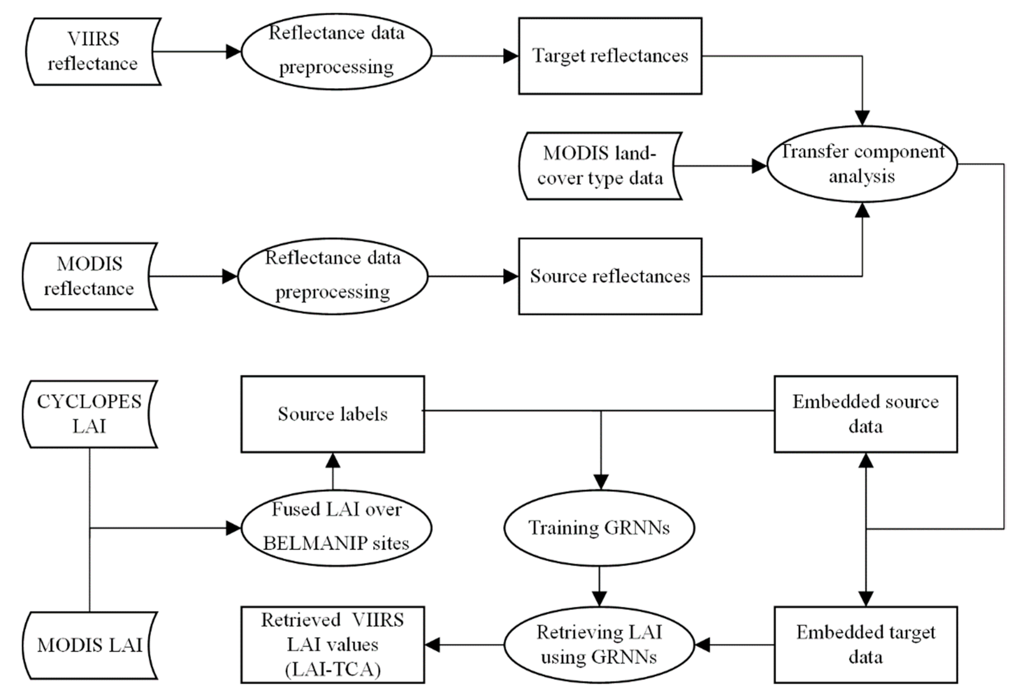
Although many studies have focused on the application of TL algorithms for classification problems, TL algorithms have rarely been used in regression problems and have not been applied to estimate biophysical parameters from satellite observations. In this paper, we intend to propose an unsupervised DA-based method to retrieve LAI values from the VIIRS surface reflectance dataset based on the training dataset that was constructed from the MODIS surface reflectance dataset. The MODIS and VIIRS surface reflectances were first mapped to the same subspace to calculate the embedded datasets through the TCA algorithm. Then, GRNNs were trained by the embedded dataset drawn from the MODIS surface reflectance dataset and the LAI values produced by fusing the MODIS and CYCLOPES products. Eventually, the trained GRNNs were utilized to estimate LAI values from the embedded data drawn from the VIIRS surface reflectance dataset.

The organization of this paper is as follows. Section 2 explains the method used for LAI retrieval, including the TCA and GRNNs, and provides an introduction to the experimental data used in this research. What is presented in Section 3 are the comparisons of the retrieved VIIRS LAI values with the TCA method and without the TCA method, the VIIRS and MODIS LAI product and the reference LAI values acquired from high-resolution reference maps. In addition, discussions and conclusions drawn are in Section 4 and Section 5, respectively.

2. Materials and Methods

The LAI retrieval method based on DA proposed in this study transfers the knowledge learned from the training dataset, which was constructed from the MODIS surface reflectance dataset for generating the GLASS LAI product, to retrieve LAI values from the VIIRS surface reflectance dataset. Figure 1 shows the flowchart of this LAI retrieval method. The training dataset constructed to generate the GLASS LAI product was composed of the preprocessed MODIS surface reflectance dataset and the LAI labels produced by fusing the MODIS and CYCLOPES products over the BELMANIP site. This training dataset was defined as the source dataset. Meanwhile, the preprocessed VIIRS surface reflectance dataset was defined as the target dataset in this paper. For reducing the discrepancies between the probability distributions of the MODIS and VIIRS surface reflectances, a TCA algorithm was used to map the source reflectances and the target reflectances to the same subspace to obtain the embedded datasets. The embedded data drawn from the MODIS surface reflectance dataset and the LAI labels produced by fusing the MODIS and CYCLOPES products were used to train the GRNNs for each biome type in a day of year. Then, for retrieving LAI values, the embedded target dataset drawn from the VIIRS surface reflectance dataset was input into the trained GRNNs. We refer to the LAI inversion results with the TCA method as LAI-TCA in this research.

2.1. Domain Adaptation via Transfer Component Analysis

The DA is able to achieve the transfer and sharing of knowledge between source domain and target domain. In this paper, the TCA algorithm is adopted, which was developed by [27] and is exclusively defined for DA. The labels of the source domains are not used for the TCA algorithm and no labels are used in the target domain. Therefore, it is an unsupervised DA method. The TCA algorithm aims to determine the common embedding of the source domain and target domain through the following two requirements: a) to minimize the probability distribution discrepancy between the source dataset and the target dataset in the reproducing kernel Hilbert space (RKHS) and b) to maximize the variance of the extracted orthogonal components.

Let $D_S=\left\{\left(x_{S1}, y_{S1}\right),\dots ,\left(x_{Sn}, y_{Sn}\right)\right\}$ be the large volume of the labelled source domain dataset, where $x_{Si}\in X_S$ is the attribute of this dataset and $y_{Si}\in Y_S$ is the corresponding label, and let $D_T=\left\{x_{T1},\dots ,x_{Tm}\right\}$ be the unlabeled target domain dataset, where $x_{Ti}\in X_T$. The distributions of the source domain and target domain are generally inconsistent. The key assumption of DA is that the marginal distribution of X_S from the source domain (P(X_S)) is different from the marginal distribution of X_T from the target domain (P(X_T)). However, the purpose of DA approaches is to estimate the target domain label by a source domain dataset. Consequently, a function $\phi (.)$ is needed to map the source domain and target domain into the same subspace and make the probability distributions of $X_S^{*}=\phi \left(X_S\right)$ and $X_T^{*}=\phi \left(X_T\right)$ as close as possible; that is, $P(X_S^{*})=P\left(X_T^{*}\right)$.

To measure the probability distribution difference between domains under the same subspace, the maximum mean discrepancy (MMD) is introduced for TCA [28]. The MMD is designed by calculating the difference of mean values between domains in the RKHS. The empirical formula of the MMD between the distribution of $X_S^{*}$ and that of $X_T^{*}$ is as follows:

$$\mathrm{MMD}\left(X_S^{*},X_T^{*}\right)=\Vert \frac{1}{n_S}{\displaystyle \sum }_{i=1}^{n_S}\phi \left(x_S\right)-\frac{1}{n_T}{\displaystyle \sum }_{i=1}^{n_T}\phi \left(x_T\right){\Vert }_{\mathrm{H}}^2$$

(1)

where $n_S$ and $n_T$ are the sample number of the source dataset and that of the target dataset, respectively. ${\Vert ·\Vert }_{\mathrm{H}}^2$ is the square module (2-norm) computed in the RKHS, which represents the square of the distance between the sample means. This quantity is close to zero if the distributions of the source dataset and target dataset tend to be exactly the same.

The key of the MMD method is to solve the mapping function $\phi (.)$. Generally, the mapping function $\phi (.)$ is highly nonlinear. It is very difficult to compute the distance between the source domain and target domain directly. Thus, the kernel trick is introduced into the quadratic term of the MMD formula. Then, Equation (1) is further rewritten as:

$$\mathrm{MMD}\left(X_S^{*},X_T^{*}\right)=tr\left(KL\right)$$

(2)

where $K=\left[\begin{array}{cc}{K}_{S,S}& K_{S,T}\\ K_{T,S}& K_{T,T}\end{array}\right]$, $K_{S,S}$, $K_{S,T}$, $K_{T,S}$, and $K_{T,T}$ are kernel matrices that reflect the similarity of samples in the source domain, target domain and cross domain. The elements $k_{i,j}=\phi {\left(x_i\right)}^T\phi \left(x_j\right)$. In addition, L is the distribution discrepancy matrix. If $x_i,x_j\in X_S$, $L_{ij}=\frac{1}{n_S^2}$; if $x_i,x_j\in X_T$, $L_{ij}=\frac{1}{n_T^2}$; otherwise, $L_{ij}=\frac{1}{n_S{n}_T}$. Alternative kernel functions K include the linear kernel, Gauss kernel, Laplace kernel, etc. The Gaussian kernel $K_{i,j}=\exp \left(\frac{-d_{ij}^2}{2a^2}\right)$,$d_{i,j}=\Vert x_i-x_j\Vert$, with the kernel bandwidth a parameter defined as the median of Euclidean distances among the data points [26], was employed to form the K matrix in this paper.

To optimize the algorithm, the dimensionality reduction method is used for MMD. The kernel matrix K can be decomposed into K = (KK^−1/2)/(K^−1/2K). The matrix $\tilde{W}\in R^{\left(n_s+n_t\right)\times m}$ is defined so that the kernel function is mapped into the m-dimensional space (m ≤ n_s + n_t). The kernel matrix K is further transformed into:

$$\tilde{K}=\left(K{K}^{-\frac{1}{2}}\tilde{W}\right)\left(\tilde{W}{K}^{-\frac{1}{2}}K\right)=KW{W}^{T}K$$

(3)

where $\tilde{K}$ is a temporary variable and $W=K^{-\frac{1}{2}}\tilde{W}$ is the transformation matrix to empirically estimate the mapping function φ. The MMD between the mapped datasets is further rewritten as:

$$\mathrm{MMD}\left(X_S^{*},X_T^{*}\right)=tr\left(\left(KW{W}^{T}K\right)L\right)=tr\left(W^{T}KLKW\right)$$

(4)

Thus, the objective illustrated in (a) is achieved by minimizing Equation (4). On the other hand, objective (b) demands that the original data characteristics that are useful to supervise the target learning can be preserved. Thus, the transformation matrix W should and can maximize the data variance in the subspace. The variance matrix ${{\displaystyle \sum }}^{*}$ of the mapped samples is quantitatively calculated by:

$${{\displaystyle \sum }}^{*}=\frac{1}{n_S+n_T}{{\displaystyle \sum }}_{i,j=1}^{n_S+n_T}\left(x_i^{*}-{\overline{x}}^{*}\right){\left(x_j^{*}-{\overline{x}}^{*}\right)}^T=W^{T}KHKW$$

(5)

where $x^{*}$ are the mapped samples and ${\overline{x}}^{*}$ is its mean. $H=I-\frac{I{I}^T}{n}$ is the centering matrix and I is the column vector whose element value is one.

According to the above deduction, the final optimization objective of the TCA algorithm based on an unsupervised domain adaptation is summarized as follows:

$$\underset{W}{\min }\{tr(\left(KW{W}^{T}K\right)L+\mu tr\left(W{W}^T\right)\}$$

$$s.t.{{\displaystyle \sum }}^{*}=W^{T}KHKW=I$$

(6)

where I is the unit matrix. The regularization term $tr\left(W^{T}W\right)$ is generally required to dominate the complexity of W. μ is the tradeoff parameter to regulate the effect of $tr\left(W^{T}W\right)$. The transformation matrix W can be solved by eigen decomposition of ${\left(KLK+\mu I\right)}^{-1}KHK$, and the W solutions are the m leading eigenvectors. After the transformation matrix W is calculated, it is allowed to compute the embedded data with m dimensions in the subspace as $X^{*}=KW$. For the detailed derivation of the TCA algorithms, please refer to [27,29].

2.2. LAI Inversion Using GRNNs

In this study, GRNNs were employed to retrieve LAI values from the embedded data extracted from the preprocessed VIIRS surface reflectance dataset. For each of the MODIS biome classes in a day of year, the GRNNs were trained by the embedded data and the fused LAI values, which are both over the BELMANIP sites. Here, the embedded data are obtained from the preprocessed MODIS surface reflectance dataset by the TCA method, and the fused LAI values are produced from the MODIS and CYCLOPES products.

2.2.1. Training Dataset

To realize the knowledge transfer between different reflectance products, a sample dataset, which was generated by [15] and was used to establish the training dataset from MODIS surface reflectance dataset for producing the GLASS LAI product, was defined as the source dataset. This dataset is composed of the LAI values produced by fusing the MODIS and CYCLOPES products and the preprocessed MODIS surface reflectance dataset that include red, near-infrared, blue, green and two shortwave infrared with center wavelengths of 1.64 µm and 2.13 µm at the BELMANIP sites from 2001 to 2003. In addition, the preprocessed VIIRS surface reflectance dataset was defined as the target dataset. To map the source and target datasets to the same subspace, the TCA algorithm was used. Thus, in this study, the embedded data obtained from the source dataset and the fused LAI values constituted the training dataset and were employed to train GRNNs.

2.2.2. General Regression Neural Networks

Figure 2 shows the GRNN architecture used for LAI retrieval. A GRNN contains four layers. They are the input layer, the pattern layer, the summation layer and the output layer. The number of neurons in the input layer is the same as the number of training samples and the transmission function is linear. The pattern layer is fully connected with the input layer, but there is no internal connection, and the transfer function is a radial basis function. The summation layer consists of two neurons. A neuron is a simple arithmetic summation of all output values of the pattern layer. The connection weight between the neurons in the pattern layer and the summation layer is 1. The other neuron is the weighted sum of all the output values of the pattern layer, and the weight is the output value of the corresponding training sample. The second neuron of the summation layer is divided by the first neuron to obtain the output value of the output layer.

The GRNNs are based on a probability density function. The common activation function of the GRNNs is the Gaussian kernel function. The estimating formula of GRNNs is deduced as follows [30]:

$$\widehat{y}\left(x\right)=\frac{{{\displaystyle \sum }}_{i=1}^n{y}_{i}exp\left[-\frac{{\left(x-x_i\right)}^T\left(x-x_i\right)}{2{\sigma }^2}\right]}{{{\displaystyle \sum }}_{i=1}^{n}exp\left[-\frac{{\left(x-x_i\right)}^T\left(x-x_i\right)}{2{\sigma }^2}\right]}$$

(7)

where $x_i$ is the input vector of the $i_{th}$ training sample and $y_i$ is the output vector of that. x is the input vector of the GRNNs and $\widehat{y}\left(x\right)$ is the output vector corresponding to the input vector x.

In this study, the input vector x employed to estimate the VIIRS LAI values contains the m dimension data obtained from the preprocessed VIIRS surface reflectance dataset and the output vector $\mathrm{y}$ is the estimated LAI values. The training input vector $x_i$ is comprised of the m dimension data gained from the preprocessed MODIS surface reflectance dataset and $y_i$ is the LAI values produced by fusing the MODIS and CYCLOPES products. According to the analysis in Section 4 the dimension m is set to 2. The n is the number of training samples. The σ is a unique parameter of the GRNN, namely the smoothing parameter. Moreover, the GRNN needs no iterative training. Thus, the GRNN has a fast learning speed. To construct a cost function for solving the optimal smoothing parameter σ, the holdout method was utilized in this paper [14].

2.3. Data and Preprocessing

2.3.1. VIIRS Reflectance Product

The VIIRS surface reflectance dataset product used in this paper is the VNP09A1 product [31], and the reflectances in the red, blue, green, near infrared and two shortwave infrared bands with center wavelengths of 1.61 µm and 2.255 µm from this product were selected. The spatial resolution of this product is 1 km and the temporal resolution of that is 8 days. It is given a sinusoidal projection and has been available since 2012.

Surface reflectances were estimated from top-of-atmosphere (TOA) reflectances through atmospheric corrections. Although great efforts were made, cloudy pixels remained in the VIIRS surface reflectances. Residual cloud and aerosol contamination results that the inconsistencies of space-time in downstream products of the VIIRS surface reflectance dataset. Therefore, it is fundamentally important to make time-series surface reflectances consistent and gap-filled. The temporally continuous vegetation index-based, land-surface reflectance dataset reconstruction (VIRR) method developed by [32] was applied to reconstruct the time-series surface reflectances from the VNP09A1 product in this study. The VIIRS surface reflectances were utilized to compute vegetation indices, and the upper envelopes of these vegetation indices were reconstructed to detect cloud-contaminated surface reflectances. Then, with the upper envelopes of the vegetation indices as constraints, the time series of surface reflectances were reconstructed from cloud-contaminated surface reflectances. For a surface reflectance dataset with multiple bands, the VIRR method simultaneously reprocesses them. Hence, it can avert inconsistencies between estimated surface reflectances at different bands. In this study, the reconstructed VIIRS surface reflectances were utilized to retrieve LAI values.

2.3.2. MODIS and VIIRS LAI Products

The MODIS LAI product Collection 6 (MCD15A2H) produced since 2002 [33] and the VIIRS LAI product (VNP15A2H) provided for the period from 2012 to the present [34] were used to evaluate the retrieved LAI values. These two LAI products with a 500 m spatial resolution and an 8-day temporal sampling period are all given a sinusoidal projection.

The MODIS and VIIRS LAI retrieval algorithms consist of a main algorithm and a backup algorithm. The inputs of this retrieval algorithm include bidirectional reflectance factors of the red and near-infrared bands, their uncertainties, sun-target-sensor geometry and a land-cover classification map. The main algorithm depends on the 3D radiative transfer model that was used to construct sensor-specific look-up tables. The backup algorithm depends on an empirical relationship between the Normalized Difference Vegetation Index (NDVI) and LAI. The backup algorithm is utilized to estimate LAI values if the main algorithm results in failure [33]. In this paper, the MODIS and VIIRS LAI values retrieved by the main algorithm and the backup algorithm all are considered to compare with our retrieved results.

Moreover, the MODIS and VIIRS LAI products provide quality control (QC) datasets for users to consult the quality information. To avoid the influence of cloud contamination on the direct validation results, the LAI values contaminated by cloud are considered as invalid values according to the QC datasets.

2.3.3. Field LAI

To validate the retrieved LAI values, the SouthWest_1, Collelongo, Capitanata, Peyrousse, 25de_Mayo_Shurb and Albufera sites with LAI reference maps from the Implementing Multiscale Agricultural Indicators Exploiting Sentinels (IMAGINES) project were selected in this paper [35]. These sites involve four vegetation types according to the MODIS land-cover type data (MCD12Q1), including broadleaf crop, grasses/cereal crop, shrub and deciduous broadleaf forest. The detailed characteristics of these sites are given in

Table 1. Characteristics of the six selected sites.

Site Name	Country	Latitude (°)	Longitude (°)	Main Biome Type	Date of LAI Reference Maps (DOY/Year)
SouthWest_1	France	43.55	1.09	Broadleaf crop	230/2013
Collelongo	Italy	41.85	13.59	Deciduous broadleaf forest	268/2015
Capitanata	Italy	41.46	15.49	Grasses/cereal crop	113/2015
Peyrousse	France	43.67	0.22	Broadleaf crop	174/2015
25de_Mayo_Shurb	Argentina	−37.94	−67.79	Shrub	40/2014
Albufera	Spain	39.27	−0.32	Grasses/cereal crop	219/2014

, including geographic coordinates, biome type, the day of year (DOY) and year of LAI reference maps. The size of these LAI reference maps is 5 km $\times$ 5 km. These maps have a 30 m or 10 m spatial resolution and are given a Universal Transverse Mercator (UTM) projection. In this research, the LAI reference maps were aggregated to a spatial resolution of 1 km over a 5 km $\times$ 5 km region, and the UTM projection of these LAI reference maps was converted to the sinusoidal projection, which is the same as the projection of the VIIRS and MODIS LAI products.

3. Results

The retrieval method based on an unsupervised DA was applied to retrieve the VIIRS LAI values in this paper. The performance of this LAI retrieval method was evaluated by comparing the retrieved LAI values with the VIIRS and MODIS LAI products with a 500 m spatial resolution and the LAI values acquired from high-resolution reference maps over the selected sites. To reasonably evaluate the retrieval results, the spatial resolution of the VIIRS and MODIS LAI products were upsampled to 1 km using the nearest neighbor resampling method. For comparison, the GRNNs trained with the MODIS surface reflectances and the LAI values produced by fusing the MODIS and CYCLOPES products were directly used to derive LAI values from the VIIRS surface reflectances without TCA. The inversion results without the TCA method are denoted by LAI-GRNN.

Figure 3 shows the temporal trajectories of the LAI-TCA and the LAI-GRNN for the SouthWest_1 site. By the MODIS land-cover classification data, the biome class of this site is the broadleaf crop. For comparison, the VIIRS and MODIS LAI values and their NDVI values calculated from the raw reflectances are also shown in Figure 3. The VIIRS and MODIS LAI values marked by the circles in Figure 3 are retrieved by the main algorithm (MA). The trajectories of the LAI-TCA and the LAI-GRNN display a similar seasonality to the trajectories of the VIIRS and MODIS LAI values. Moreover, the time series of the LAI-TCA and that of the VIIRS NDVI values have consistent seasonal variation. The discrepancy between the temporal trend of the LAI-TCA and that of the LAI-GRNN is slight. However, the LAI-TCA is universally higher than the LAI-GRNN. During the nongrowing season, the LAI-TCA and LAI-GRNN are agree well with the VIIRS LAI values. Nevertheless, during the growing season, the LAI-TCA and LAI-GRNN are obviously lower than the VIIRS LAI values and the quality of the VIIRS LAI values retrieved by the backup algorithm is poor. These LAI values shown in Figure 3 are all evidently smaller than the reference LAI value. However, the estimated LAI-TCA is more approximate to the reference LAI value than the LAI-GRNN.

Figure 4 shows the LAI-TCA in a 5 km $\times$ 5 km SouthWest_1 site areas on Day 230, 2013. Figure 4a,b show that the images of the LAI-TCA and the LAI-GRNN have very similar distribution trends. The map of the LAI-TCA has a similar variation pattern to the reference LAI map in this region, especially in the northwestern corner and southwestern corner. The LAI-TCA values are generally higher than the VIIRS and MODIS LAI values. Nevertheless, the LAI-TCA values are highly consistent with the reference LAI values compared with the VIIRS and MODIS LAI values. In addition, there are obvious differences between these LAI images in the middle where the LAI-TCA and LAI-GRNN values and the VIIRS and MODIS LAI values are underestimated comparing to the reference LAI values.

Figure 4f–i demonstrate the statistical distributions of discrepancies between the LAI-TCA, the LAI-GRNN, the VIIRS and MODIS LAI values and the reference LAI values at the SouthWest_1 site. The standard deviation of the discrepancies between the LAI-TCA and the reference LAI values is 0.31, while that of the discrepancies between the LAI-GRNN, the VIIRS and MODIS LAI values and the reference LAI values are 0.34, 0.49 and 0.43, respectively. This indicates that the discrepancies between the LAI-TCA and the reference LAI values have a more concentrated distribution. The mean value of the discrepancies between the LAI-TCA and the reference LAI values are also lower than that of the discrepancies between the LAI-GRNN, the VIIRS and MODIS LAI values and the reference LAI values.

To a certain extent, these phenomena indicate that the LAI-TCA are more consistent with the reference LAI values than the LAI-GRNN and the VIIRS and MODIS LAI values, although the LAI-TCA are slightly underestimated at this site.

Figure 5 depicts the temporal trajectories of the LAI-TCA and the LAI-GRNN for the Collelongo site with the deciduous broadleaf forest biome class. During the growing season, these trajectories all exhibited fluctuations and fluctuations of the LAI-GRNN trajectory, the VIIRS LAI trajectory and the MODIS LAI trajectory were stronger than those of the LAI-TCA trajectory. During the nongrowing season, the trends of these trajectories were more consistent. On Julian Day 329, the VIIRS and MODIS LAI values decrease markedly because of the influence of the cloud-contaminated VIIRS and MODIS reflectances. However, the LAI-TCA and LAI-GRNN values have no fluctuation on this Julian day. Moreover, the LAI-TCA outperforms the LAI-GRNN and the VIIRS and MODIS LAI values in comparison with the reference LAI value at this site.

Figure 6 shows images of the LAI-TCA, the LAI-GRNN, and the VIIRS and MODIS LAI values at the Collelongo site on Day 266, 2015. By analyzing these images, it can be observed that from the southwestern corner to the northeastern corner, the LAI-TCA agrees with the reference LAI values. In the east and west, the LAI-TCA has a slight underestimation comparing to the reference LAI values. The distributions of the LAI-TCA and LAI-GRNN are generally uniform in this area, except for the center where the LAI-GRNN are usually higher than the LAI-TCA. However, there are more LAI values that are apparently underestimated in the VIIRS LAI map, particularly when the reference LAI values are relatively low.

Figure 6f–i demonstrate the statistical distributions of the discrepancy between the LAI-TCA, the LAI-GRNN, the VIIRS and MODIS LAI values and the reference LAI values at the Collelongo site. Discrepancies between the LAI-TCA and reference LAI values are more concentrated with a smaller standard deviation of 0.62 than discrepancies between the VIIRS LAI values and reference LAI values with a standard deviation of 1.43 and discrepancies between the MODIS LAI values and reference LAI values with a standard deviation of 0.98. The range of discrepancies between LAI-TCA and reference LAI is −1.0~1.37, whereas the range of discrepancies between VIIRS LAI and reference LAI is −2.38~2.01 and the range of discrepancies between MODIS LAI and reference LAI is −2.2~1.31. Furthermore, the mean value of the discrepancies between the LAI-TCA and the reference LAI values are lowest. Thus, discrepancies between the estimated LAI-TCA map and reference LAI map are smaller.

The LAI-TCA, the LAI-GRNN, and the VIIRS and MODIS LAI temporal trajectories at the Capitanata site with the grasses/cereal crop biome class are shown in Figure 7. From Day 129 to Day 153, the LAI-TCA and LAI-GRNN values are significantly higher than the MODIS LAI values. However, the VIIRS and MODIS NDVI values calculated from the raw reflectances show no significant difference in this period, and the LAI-TCA and LAI-GRNN are retrieved from the preprocessed VIIRS surface reflectance dataset. Thus, this discrepancy may be caused by the discrepancies between the preprocessed VIIRS and MODIS surface reflectances. In the other periods, the LAI-TCA has a similar seasonality to the VIIRS and MODIS LAI values. Moreover, the LAI-TCA temporal trajectory has a smoother trend than the VIIRS LAI temporal trajectory. At this site, the LAI-TCA is more approximate to the reference LAI value than the LAI-GRNN.

Figure 8 shows images of the LAI-TCA, the LAI-GRNN, and the VIIRS and MODIS LAI values at the Capitanata site on Day 113, 2015. It can be clearly seen from these images that for the majority of pixels, the VIIRS LAI values are lower than the reference LAI values. In addition, the LAI-GRNN values are slightly lower than the reference LAI values in the north. Surprisingly, the spatial distribution of the LAI-TCA is relatively consistent with the reference LAI values.

Figure 8f–i demonstrate the statistical distributions of the discrepancy between the LAI-TCA, the LAI-GRNN, the VIIRS and MODIS LAI values and the reference LAI values at the Capitanata site. Compared with the discrepancy between the LAI-GRNN, the VIIRS and MODIS LAI values and the reference LAI values, the discrepancy between the LAI-TCA and reference LAI values has a lower standard deviation (0.51). Moreover, the distribution of the discrepancies between the LAI-TCA and reference LAI values is more concentrated than that of the discrepancies between the LAI-GRNN, the VIIRS and MODIS LAI values and the reference LAI values.

Figure 9 displays the temporal trajectories of the LAI-TCA and the LAI-GRNN for the Peyrousse site with the broadleaf crop biome class. Good temporal consistency is realized among these temporal trajectories during the nongrowing season. Nevertheless, the LAI-TCA and the LAI-GRNN values are slightly larger than the MODIS LAI values throughout almost the entire year, except for the period from Day 209 to Day 241. On Julian Days 81 and 113, the VIIRS LAI values are obviously affected by cloud contamination. However, the LAI-TCA and LAI-GRNN values have no mutations on these two Julian days. This is because the LAI-TCA and LAI-GRNN were retrieved from the elimination-cloud-contaminated VIIRS surface reflectance dataset. At this site, the LAI-TCA is nearer to the reference LAI value comparing to the LAI-GRNN.

Figure 10 shows images of the LAI-TCA, the LAI-GRNN, and the VIIRS and MODIS LAI values at the Peyrousse site on Day 174, 2015. The spatial distributions of these images are approximate and show a decreasing trend from west to east. The values of these images have a great difference in the southwestern corner where the LAI-TCA and TCA-GRNNs and the VIIRS and MODIS LAI values all exceed the reference LAI values.

Figure 10f–i demonstrate the statistical distributions of the discrepancy between the LAI-TCA, the LAI-GRNN, the VIIRS and MODIS LAI values and the reference LAI values at the Peyrousse site. The discrepancy between the LAI-TCA and reference LAI values has a lower standard deviation (0.36) than the discrepancy between the LAI-GRNN, the VIIRS and MODIS LAI values and the reference LAI values. Moreover, compared with discrepancies between the LAI-GRNN, the VIIRS and MODIS LAI values and the reference LAI values, discrepancies between the LAI-TCA and the reference LAI values have a smaller range. Thus, the LAI-TCA values are in better agreement with the reference LAI values than the VIIRS and MODIS LAI values.

Figure 11 displays the temporal trajectories of the LAI-TCA and the LAI-GRNN for the 25de_Mayo_Shurb site with the shrub biome type. These trajectories all exhibit limited seasonality. From Day 41 to Day 81, the discrepancy between the retrieved LAI and MODIS LAI trajectories is consistent with the discrepancy between the VIIRS and MODIS NDVI trajectories. From Day 281 to Day 361, the MODIS NDVI values are lower than the VIIRS NDVI values, but the LAI-TCA are lower than the MODIS LAI, which demonstrates that the LAI-TCA are easily affected by the reflectances of bands except the red band and near-infrared band at this site with sparse vegetation.

Figure 12 shows images of the LAI-TCA, the LAI-GRNN, and the VIIRS and MODIS LAI values at the 25de_Mayo_Shurb site on Day 40, 2014. The LAI values of these images show similar spatial patterns. However, in the west, there are some observable discrepancies.

Figure 12f–i demonstrate the statistical distributions of the discrepancy between the LAI-TCA, the LAI-GRNN, the VIIRS and MODIS LAI values and the reference LAI values at the 25de_Mayo_Shurb site. The range of discrepancies between LAI-TCA and reference LAI is −0.36~0.75, but the range of discrepancies between LAI-GRNN and reference LAI is −0.72~0.62, the range of discrepancies between VIIRS LAI and reference LAI is −0.49~1.09 and the range of discrepancies between MODIS LAI and reference LAI is −1.18~0.33. Moreover, the standard deviation (0.25) of the discrepancy between LAI-TCA and reference LAI is lower than that of the discrepancy between LAI-GRNN, VIIRS and MODIS LAI and the reference LAI. Thus, the LAI-TCA has fewer discrepancies with the reference LAI.

Figure 13 displays the temporal trajectories of the LAI-TCA and the LAI-GRNN for the Albufera site with the grasses/cereal crop biome type. These trajectories all show normal seasonal changes. During the growing season, the peak values of the LAI-TCA, LAI-GRNN and VIIRS LAI temporal trajectories are apparently lower than that of the MODI LAI temporal trajectory. On Day 217, the LAI-TCA, the LAI-GRNN and the VIIRS LAI that from the VIIRS surface reflectance are lower than the reference LAI value. However, comparing to the LAI-GRNN, the LAI-TCA is nearer to the reference LAI value.

Figure 14 shows images of the LAI-TCA, the LAI-GRNN, and the VIIRS and MODIS LAI values at the Albufera site on Day 219, 2014. At this site, the LAI-TCA and the LAI-GRNN have a small discrepancy. The LAI-TCA and the LAI-GRNN are generally less than the reference LAI values, but the spatial distribution of these values is concentrated as the reference LAI values. However, many VIIRS and MODIS LAI values are higher than the reference LAI values and the spatial distribution of these values is obviously discrete.

Figure 14f–i demonstrate the statistical distributions of the discrepancy between the LAI-TCA, the LAI-GRNN, the VIIRS and MODIS LAI values and the reference LAI values at the Albufera site. The range of discrepancies between LAI-TCA, LAI-GRNN and reference LAI are significantly less than that between VIIRS LAI, MODIS LAI and reference LAI. The standard deviation (0.5) of the discrepancy between LAI-TCA and reference LAI is evidently smaller than that of the discrepancy between VIIRS and MODIS LAI and the reference LAI. The standard deviation of the discrepancy between LAI-TCA, LAI-GRNN and reference LAI is approximate, but the range and mean of discrepancies between LAI-TCA and reference LAI are lower than these of discrepancies between LAI-GRNN and reference LAI. Hence, the LAI-TCA values have a better consistency with the reference LAI values.

Figure 15 demonstrates the scatter plots of the LAI-TCA, the LAI-GRNN, the VIIRS and the MODIS LAI values versus the reference LAI values at all selected sites. The VIIRS and the MODIS LAI values contaminated by cloud have been removed. The slope of the regression line for the LAI-TCA versus the reference LAI values is 0.78. This reveals that the LAI-TCA slightly overestimate the reference LAI values along with low values and underestimate the reference LAI values along with high values. Despite all this, the correlation of the LAI-TCA and LAI reference values (R² = 0.88) outperforms that of the LAI-GRNN, the VIIRS LAI product and the MODIS LAI product. In addition, the LAI-TCA (RMSE = 0.68) provide better accuracy than the LAI-GRNN, the VIIRS LAI product and the MODIS LAI product. These results demonstrate that the retrieval results with the TCA method is in a better consistency with the reference LAI values than the LAI-GRNN and the VIIRS and MODIS LAI products.

4. Discussion

The source dataset and target dataset defined in this paper contain the preprocessed MODIS and VIIRS surface reflectance dataset of six bands. Therefore, the maximum dimension of the embedded dataset m is 6. The impact of different dimensions on the LAI inversion performances must be discussed. By analyzing the mean RMSE and R² values of the results for different dimensions over selected sites in Figure 16, it can be seen that the number of dimensions has a significant influence on the inversion accuracy. When the number of dimensions is 2, it is obvious that the inversion performance is best, with the lowest mean RMSE value of 0.65 and the highest mean R² value of 0.54. However, the inversion accuracy apparently decreases when the number of dimensions is larger than 2. This phenomenon, called the “curse of dimensionality”, is due to the significant sparsity of the high-dimensional spatial distribution. This problem can be solved by reducing the number of dimensions on account of redundant information included in feature components [36]. Therefore, the optimum number of dimensions should be 2 in this paper.

In this study, the results of the LAI-TCA are good in spatial distribution and time series. Meanwhile, the LAI-TCA with the processing of transfer learning is better than the LAI-GRNN without that. In order to improve the accuracy of inversion, the training dataset used to train GRNNs is separated by biome type and day of year. Hence, from Figure 15, the performance of retrieved LAI is promoted comparing to the VIIRS LAI product and the MODIS LAI product.

The advantage of the LAI retrieved method proposed in this paper is that it can directly use the existing training dataset constructed by the MODIS surface reflectances and use the transfer learning method to obtain LAI values from other sensor data with a good quality. It should be noted that the period of the existing training dataset from 2001 to 2003 is different from that of the VIIRS surface reflectances since 2012, in this study. However, comparing Figure 15a,b, the accuracy of the retrieved LAI values based on transfer learning can be slightly improved. The difference shown in Figure 15a,b is sufficient to illustrate that there is a difference in the distribution of MODIS surface reflectances and VIIRS surface reflectances. Thus, when using the existing training dataset to retrieve LAI product from other sensors, it is necessary to transfer knowledge. Moreover, the transfer learning method can realize positive transfer under the context proposed in this paper.

In Section 3 the retrieved LAI values are cross validated and directly validated. The vegetation type of these selected sites for validation includes different biome types, namely forest, shrub, grass and crop. The MODIS surface reflectances as the source domain and the VIIRS surface reflectances as the target domain in this paper are processed to eliminate the influence of cloud by the same method. In addition, design of the VIIRS was quite similar to the MODIS [37]. To some extent, this leads to no significant difference between Figure 15a,b.

The method proposed in this paper is an exploratory experiment of applying transfer learning to parameter inversion. At the same time, it is a knowledge transfer method based on data. In further work, we will use the model-based transfer learning method to retrieve biophysical parameters, so as to build a more convenient, better and faster unified inversion platform. The application of transfer learning in the parameter inversion field is not limited to reducing the difference in data distribution from different sensors. Aiming at the problem that the geographic information deviation of Chinese satellite data affects the retrieval accuracy [38], transfer learning can be used to improve retrieval accuracy. Furthermore, the transfer learning method can also transfer the reflectance data information with different spatiotemporal scales for inversion of parameter products with high spatiotemporal resolution. Transfer learning methods have great application value and potential, whether used to build a unified training dataset and model for inversion of LAI parameters from different sensors, or to acquire parameter products with high spatiotemporal resolution.

5. Conclusions

This study develops a retrieval method based on an unsupervised DA to obtain LAI values from VIIRS surface reflectance. The TCA method for DA is used to minimize discrepancies of probability distributions between the MODIS and VIIRS surface reflectances to obtain the embedded datasets in the same subspace. The GRNNs are trained by the embedded data that are extracted from preprocessed MODIS surface reflectance dataset and the LAI values produced by fusing the MODIS and CYCLOPES products, and then the trained GRNNs are employed to retrieve LAI values from the embedded data extracted from the preprocessed VIIRS surface reflectances. The performance evaluation of the LAI-TCA is conducted at selected sites. The results demonstrate that the temporal trajectories of LAI-TCA show a similar seasonality to those of the VIIRS and MODIS LAI values, and their spatial distributions are well-consistent with the reference LAI values. Moreover, the LAI-TCA with the R² 0.88 and the RMSE 0.68 are more consistent with the LAI values acquired from high-resolution reference maps than the LAI-GRNN, VIIRS and MODIS LAI values.

In this study, TL between MODIS and VIIRS sensor observations is realized by the TCA method based on unsupervised domain adaptation. Given a constructed sample dataset, this method can be further employed to retrieve LAI values from other sensor observations, such as AVHRR, VEGETATION and FengYun. Furthermore, this method can also be used to retrieve other biophysical parameters, such as fractional vegetation cover (FVC), fraction of absorbed photosynthetically active radiation (FAPAR) and albedo. In our future research, more extensive validation will be undertaken to verify the effectiveness of this proposed method.

References

1. García-Haro, F.J.; Campos-Taberner, M.; Muñoz-Marí, J.; Laparra, V.; Camacho, F.; Sánchez-Zapero, J.; Camps-Valls, G. Derivation of global vegetation biophysical parameters from EUMETSAT Polar System. ISPRS J. Photogramm. Remote Sens. 2018, 139, 57–74. [Google Scholar] [CrossRef]
2. Lakshmi, V.; Wood, E.F.; Choudhury, B.J. Simulation of microwave brightness temperatures using a coupled land-surface-canopy-atmosphere model. In Proceedings of the IGARSS’94-1994 IEEE International Geoscience and Remote Sensing Symposium, Pasadena, CA, USA, 8–12 August 1994; IEEE: Piscataway, NJ, USA, 1994; Volume 1, pp. 590–592. [Google Scholar]
3. Heldens, W.; Esch, T.; Heiden, U. Supporting urban micro climate modelling with airborne hyperspectral data. In Proceedings of the 2012 IEEE International Geoscience and Remote Sensing Symposium, Munich, Germany, 22–27 July 2012; IEEE: Piscataway, NJ, USA, 2012; pp. 1598–1601. [Google Scholar]
4. Huang, J.; Ma, H.; Su, W.; Zhang, X.; Huang, Y.; Fan, J.; Wu, W. Jointly Assimilating MODIS LAI and ET Products Into the SWAP Model for Winter Wheat Yield Estimation. IEEE J. Sel. Top. Appl. Earth Obs. Remote Sens. 2015, 8, 4060–4071. [Google Scholar] [CrossRef]
5. Veroustraete, F.; Patyn, J.; Myneni, R. Estimating net ecosystem exchange of carbon using the normalized difference vegetation index and an ecosystem model. Remote Sens. Environ. 1996, 58, 115–130. [Google Scholar] [CrossRef]
6. Borel, C.C.; Gerstl, S.A.; Powers, B.J. The radiosity method in optical remote sensing of structured 3-D surfaces. Remote Sens. Environ. 1991, 36, 13–44. [Google Scholar] [CrossRef]
7. Chen, J.M.; Leblanc, S.G. Multiple-scattering scheme useful for geometric optical modeling. IEEE Trans. Geosci. Remote Sens. 2001, 39, 1061–1071. [Google Scholar] [CrossRef]
8. Li, X.; Strahler, A. Geometric-optical bidirectional reflectance modeling of the discrete crown vegetation canopy: Effect of crown shape and mutual shadowing. IEEE Trans. Geosci. Remote Sens. 1992, 30, 276–292. [Google Scholar] [CrossRef]
9. Luo, Z.; Luan, K.; Zhu, W.; Xia, W.; Jiang, X.; Zhu, M. Research on Empirical Model and Gap Rate Model for Estimating Rice Leaf Area Index Based on UAV HD Digital Images. In Proceedings of the 2018 7th International Conference on Agro-Geoinformatics (Agro-Geoinformatics), Hangzhou, China, 6–9 August 2018; IEEE: Piscataway, NJ, USA, 2018; pp. 1–5. [Google Scholar] [CrossRef]
10. Atzberger, C.; Richter, K. Spatially constrained inversion of radiative transfer models for improved LAI mapping from future Sentinel-2 imagery. Remote Sens. Environ. 2012, 120, 208–218. [Google Scholar] [CrossRef]
11. Yuan, Q.; Shen, H.; Li, T.; Li, Z.; Li, S.; Jiang, Y.; Xu, H.; Tan, W.; Yang, Q.; Wang, J.; et al. Deep learning in environmental remote sensing: Achievements and challenges. Remote Sens. Environ. 2020, 241, 111716. [Google Scholar] [CrossRef]
12. Baret, F.; Hagolle, O.; Geiger, B.; Bicheron, P.; Miras, B.; Huc, M.; Berthelot, B.; Niño, F.; Weiss, M.; Samain, O.; et al. LAI, fAPAR and fCover CYCLOPES global products derived from VEGETATION: Part 1: Principles of the algorithm. Remote Sens. Environ. 2007, 110, 275–286. [Google Scholar] [CrossRef] [Green Version]
13. Baret, F.; Weiss, M.; Lacaze, R.; Camacho, F.; Makhmara, H.; Pacholcyzk, P.; Smets, B. GEOV1: LAI and FAPAR essential climate variables and FCOVER global time series capitalizing over existing products. Part1: Principles of development and production. Remote Sens. Environ. 2013, 137, 299–309. [Google Scholar] [CrossRef]
14. Xiao, Z.; Liang, S.; Wang, J.; Chen, P.; Yin, X.; Zhang, L.; Song, J. Use of General Regression Neural Networks for Generating the GLASS Leaf Area Index Product From Time-Series MODIS Surface Reflectance. IEEE Trans. Geosci. Remote Sens. 2013, 52, 209–223. [Google Scholar] [CrossRef]
15. Xiao, Z.; Liang, S.; Wang, J.; Xiang, Y.; Zhao, X.; Song, J. Long-Time-Series Global Land Surface Satellite Leaf Area Index Product Derived From MODIS and AVHRR Surface Reflectance. IEEE Trans. Geosci. Remote Sens. 2016, 54, 5301–5318. [Google Scholar] [CrossRef]
16. Claverie, M.; Matthews, J.L.; Vermote, E.F.; Justice, C.O. A 30+ Year AVHRR LAI and FAPAR Climate Data Record: Algorithm Description and Validation. Remote Sens. 2016, 8, 263. [Google Scholar] [CrossRef] [Green Version]
17. Zhu, Z.; Bi, J.; Pan, Y.; Ganguly, S.; Anav, A.; Xu, L.; Samanta, A.; Piao, S.; Nemani, R.R.; Myneni, R.B. Global Data Sets of Vegetation Leaf Area Index (LAI)3g and Fraction of Photosynthetically Active Radiation (FPAR)3g Derived from Global Inventory Modeling and Mapping Studies (GIMMS) Normalized Difference Vegetation Index (NDVI3g) for the Period 1981 to 2011. Remote Sens. 2013, 5, 927–948. [Google Scholar] [CrossRef] [Green Version]
18. Franke, J.; Heinzel, V.; Menz, G. Assessment of NDVI- Differences Caused by Sensor Specific Relative Spectral Response Functions. In Proceedings of the 2006 IEEE International Symposium on Geoscience and Remote Sensing, Denver, CO, USA, 31 July–4 August 2006; pp. 1138–1141. [Google Scholar]
19. Zhong, B. Methodology for Nomalization of Optical Remote Sensing Data from Multi-Sensor; Science Press: Beijing, China, 2015. (In Chinese) [Google Scholar]
20. Pan, S.J.; Yang, Q. A Survey on Transfer Learning. IEEE Trans. Knowl. Data Eng. 2010, 22, 1345–1359. [Google Scholar] [CrossRef]
21. Zhang, J.; Li, W.Q.; Ogunbona, P. Joint Geometrical and Statistical Alignment for Visual Domain Adaptation. In Proceedings of the 30th IEEE Conference on Computer Vision and Pattern Recognition (Cvpr 2017), Honolulu, HI, USA, 21–26 July 2016; IEEE: Piscataway, NJ, USA, 2017; pp. 5150–5158. [Google Scholar] [CrossRef] [Green Version]
22. Liu, Y.; Zhang, Y.; Coleman, S.; Chi, J. Joint transfer component analysis and metric learning for person re-identification. Electron. Lett. 2018, 54, 821–823. [Google Scholar] [CrossRef] [Green Version]
23. Li, Y.; Sheng, H.; Cheng, Y.; Stroe, D.-I.; Teodorescu, R. State-of-health estimation of lithium-ion batteries based on semi-supervised transfer component analysis. Appl. Energy 2020, 277, 115504. [Google Scholar] [CrossRef]
24. Deep, S.; Zheng, X. Leveraging CNN and Transfer Learning for Vision-based Human Activity Recognition. In Proceedings of the 29th International Telecommunication Networks and Applications Conference (ITNAC), Auckland, New Zealand, 27–29 November 2019; IEEE: Piscataway, NJ, USA, 2019; pp. 1–4. [Google Scholar] [CrossRef]
25. Xia, J.; Yokoya, N.; Iwasaki, A. Ensemble of transfer component analysis for domain adaptation in hyperspectral remote sensing image classification. In Proceedings of the IEEE International Geoscience and Remote Sensing Symposium (IGARSS), Fort Worth, TX, USA, 23–28 July 2017; IEEE: Piscataway, NJ, USA, 2017; pp. 4762–4765. [Google Scholar] [CrossRef]
26. Matasci, G.; Volpi, M.; Kanevski, M.; Bruzzone, L.; Tuia, D. Semisupervised Transfer Component Analysis for Domain Adaptation in Remote Sensing Image Classification. IEEE Trans. Geosci. Remote Sens. 2015, 53, 3550–3564. [Google Scholar] [CrossRef]
27. Pan, S.J.; Tsang, I.; Kwok, J.T.; Yang, Q. Domain Adaptation via Transfer Component Analysis. IEEE Trans. Neural Netw. 2010, 22, 199–210. [Google Scholar] [CrossRef] [Green Version]
28. Borgwardt, K.M.; Gretton, A.; Rasch, M.J.; Kriegel, H.-P.; Schölkopf, B.; Smola, A.J. Integrating structured biological data by Kernel Maximum Mean Discrepancy. Bioinformatics 2006, 22, e49–e57. [Google Scholar] [CrossRef] [Green Version]
29. Chen, C.; Li, Z.; Yang, J.; Liang, B. A cross domain feature extraction method based on transfer component analysis for rolling bearing fault diagnosis. In Proceedings of the 29th Chinese Control and Decision Conference (CCDC), Chongqing, China, 28–30 May 2017; IEEE: Piscataway, NJ, USA, 2017; pp. 5622–5626. [Google Scholar] [CrossRef]
30. Specht, D.F. A general regression neural network. IEEE Trans. Neural Netw. 1991, 2, 568–576. [Google Scholar] [CrossRef] [PubMed] [Green Version]
31. Bian, J.; Li, A.; Huang, C.; Zhang, R.; Zhan, X. A self-adaptive approach for producing clear-sky composites from VIIRS surface reflectance datasets. ISPRS J. Photogramm. Remote Sens. 2018, 144, 189–201. [Google Scholar] [CrossRef]
32. Xiao, Z.; Liang, S.; Wang, T.; Liu, Q. Reconstruction of Satellite-Retrieved Land-Surface Reflectance Based on Temporally-Continuous Vegetation Indices. Remote Sens. 2015, 7, 9844–9864. [Google Scholar] [CrossRef] [Green Version]
33. Knyazikhin, Y.; Martonchik, J.V.; Myneni, R.B.; Diner, D.J.; Running, S.W. Synergistic algorithm for estimating vegetation canopy leaf area index and fraction of absorbed photosynthetically active radiation from MODIS and MISR data. J. Geophys. Res. Atmos. 1998, 103, 32257–32275. [Google Scholar] [CrossRef] [Green Version]
34. Yan, K.; Park, T.; Chen, C.; Xu, B.; Song, W.; Yang, B.; Zeng, Y.; Liu, Z.; Yan, G.; Knyazikhin, Y.; et al. Generating Global Products of LAI and FPAR From SNPP-VIIRS Data: Theoretical Background and Implementation. IEEE Trans. Geosci. Remote Sens. 2018, 56, 2119–2137. [Google Scholar] [CrossRef]
35. Li, J.; Xiao, Z. Evaluation of the version 5.0 global land surface satellite (GLASS) leaf area index product derived from MODIS data. Int. J. Remote Sens. 2020, 41, 9140–9160. [Google Scholar] [CrossRef]
36. Salimi, A.; Ziaii, M.; Amiri, A.; Hosseinjanizadeh, M.; Karimpouli, S.; Moradkhani, M. Using a Feature Subset Selection method and Support Vector Machine to address curse of dimensionality and redundancy in Hyperion hyperspectral data classification. Egypt. J. Remote Sens. Space Sci. 2018, 21, 27–36. [Google Scholar] [CrossRef]
37. Xu, B.; Park, T.; Yan, K.; Chen, C.; Zeng, Y.; Song, W.; Yin, G.; Li, J.; Liu, Q.; Knyazikhin, Y.; et al. Analysis of Global LAI/FPAR Products from VIIRS and MODIS Sensors for Spatio-Temporal Consistency and Uncertainty from 2012–2016. Forests 2018, 9, 73. [Google Scholar] [CrossRef] [Green Version]
38. Bicheron, P.; Amberg, V.; Bourg, L.; Petit, D.; Huc, M.; Miras, B.; Brockmann, C.; Hagolle, O.; Delwart, S.; Ranera, F.; et al. Geolocation Assessment of MERIS GlobCover Orthorectified Products. IEEE Trans. Geosci. Remote Sens. 2011, 49, 2972–2982. [Google Scholar] [CrossRef]
Figure 1. The LAI retrieval method based on domain adaptation.
Remotesensing 14 01826 g001
Figure 2. GRNN architecture used for LAI retrieval.
Remotesensing 14 01826 g002
Figure 3. Temporal trajectories of the LAI-TCA and LAI-GRNN at the center pixel of the SouthWest_1 site for 2013.
Remotesensing 14 01826 g003
Figure 4. Images of the LAI-TCA (a), the LAI-GRNN (b), the VIIRS (c), the MODIS (d) and the LAI values acquired from high-resolution reference maps (e) at the SouthWest_1 site on Day 230, 2013. (fi) Statistical distributions of discrepancies between the LAI-TCA, the LAI-GRNN, the VIIRS, the MODIS and the LAI values acquired from high-resolution reference maps.
Remotesensing 14 01826 g004
Figure 5. Temporal profiles of the retrieved LAI-TCA and the retrieved LAI-GRNN at the center pixel of the Collelongo site for 2015.
Remotesensing 14 01826 g005
Figure 6. Images of the LAI-TCA (a), the LAI-GRNN (b), the VIIRS (c), the MODIS (d) and the LAI values acquired from high-resolution reference maps (e) at the Collelongo site on Day 268, 2015. (fi) Statistical distributions of discrepancies between the LAI-TCA, the LAI-GRNN, the VIIRS, the MODIS and the LAI values acquired from high-resolution reference maps.
Remotesensing 14 01826 g006
Figure 7. Temporal trajectories of the LAI-TCA and the LAI-GRNN at the center pixel of the Capitanata site for 2015.
Remotesensing 14 01826 g007
Figure 8. Images of the LAI-TCA (a), the LAI-GRNN (b), the VIIRS (c), the MODIS (d) and the LAI values acquired from high-resolution reference maps (e) at the Capitanata site on Day 113, 2015. (fi) Statistical distributions of discrepancies between the LAI-TCA, the LAI-GRNN, the VIIRS, the MODIS and the LAI values acquired from high-resolution reference maps.
Remotesensing 14 01826 g008
Figure 9. Temporal trajectories of the LAI-TCA and the LAI-GRNN at the center pixel of the Peyrousse site for 2015.
Remotesensing 14 01826 g009
Figure 10. Images of the LAI-TCA (a), the LAI-GRNN (b), the VIIRS (c), the MODIS (d) and the LAI values acquired from high-resolution reference maps (e) at the Peyrousse site on Day 174, 2015. (fi) Statistical distributions of discrepancies between the LAI-TCA, the LAI-GRNN, the VIIRS, the MODIS and the LAI values acquired from high-resolution reference maps.
Remotesensing 14 01826 g010
Figure 11. Temporal trajectories of the LAI-TCA and the LAI-GRNN at the center pixel of the 25de_Mayo_Shurb site for 2014.
Remotesensing 14 01826 g011
Figure 12. Images of the LAI-TCA (a), the LAI-GRNN (b), the VIIRS (c), the MODIS (d) and the LAI values acquired from high-resolution reference maps (e) at the 25de_Mayo_Shurb site on Day 40, 2014. (fi) Statistical distributions of discrepancies between the LAI-TCA, the LAI-GRNN, the VIIRS, the MODIS and the LAI values acquired from high-resolution reference maps.
Remotesensing 14 01826 g012
Figure 13. Temporal trajectories of the LAI-TCA and the LAI-GRNN at the center pixel of the Albufera site for 2014.
Remotesensing 14 01826 g013
Figure 14. Images of the LAI-TCA (a), the LAI-GRNN (b), the VIIRS (c), the MODIS (d) and the LAI values acquired from high-resolution reference maps (e) at the Albufera site on Day 219, 2014. (f–i) Statistical distributions of discrepancies between the LAI-TCA, the LAI-GRNN, the VIIRS, the MODIS and the LAI values acquired from high-resolution reference maps.
Remotesensing 14 01826 g014
Figure 15. Scatter plots of the LAI-TCA (a), the LAI-GRNN (b), the VIIRS LAI values (c) and the MODIS LAI values (d) versus the LAI values acquired from high-resolution reference maps for the six selected sites. The black dashed lines show the uncertainty boundaries proposed by GCOS (max (0.5, 20%)) for LAI.
Remotesensing 14 01826 g015
Figure 16. Performance of the LAI-TCA considering different dimensions.
Remotesensing 14 01826 g016