Article

High-Resolution Boundary-Constrained and Context-Enhanced Network for Remote Sensing Image Segmentation

1
School of Instrumentation and Optoelectronic Engineering, Beihang University, Beijing 100191, China
2
Key Laboratory of Precision Opto-Mechatronics Technology, Ministry of Education, Beihang University, Beijing 100191, China
*
Author to whom correspondence should be addressed.
Remote Sens. 2022, 14(8), 1859; https://doi.org/10.3390/rs14081859
Submission received: 8 March 2022 / Revised: 9 April 2022 / Accepted: 10 April 2022 / Published: 12 April 2022
(This article belongs to the Special Issue Remote Sensing Image and Urban Information Visualization)

Abstract

:
The technology of remote sensing image segmentation has made great progress in recent years. However, there are still several challenges which need to be addressed (e.g., ground objects blocked by shadows, higher intra-class variance and lower inter-class variance). In this paper, we propose a novel high-resolution boundary-constrained and context-enhanced network (HBCNet), which combines boundary information to supervise network training and utilizes the semantic information of categories with the regional feature presentations to improve final segmentation accuracy. On the one hand, we design the boundary-constrained module (BCM) and form the parallel boundary segmentation branch, which outputs the boundary segmentation results and supervises the network training simultaneously. On the other hand, we also devise a context-enhanced module (CEM), which integrates the self-attention mechanism to advance the semantic correlation between pixels of the same category. The two modules are independent and can be directly embedded in the main segmentation network to promote performance. Extensive experiments were conducted using the ISPRS Vahingen and Potsdam benchmarks. The mean F1 score (m-F1) of our model reached 91.32% and 93.38%, respectively, which exceeds most existing CNN-based models and represents state-of-the-art results.

Graphical Abstract

1. Introduction

Semantic segmentation of remote sensing images plays a significant role in remote sensing image processing. It aims to classify various ground object categories in the image pixel by pixel (e.g., roads, buildings, trees, vehicles and fields) and give the corresponding semantic information. It has been widely applied in urban planning [1], environmental monitoring [2] and land resource utilization [3].
The main methods of remote sensing image segmentation are based on full convolution neural networks and involve design of an appropriate model structure to extract as much ground feature information as possible. To better integrate high-level and low-level features, UNet [4] employs skip connection and SegNet [5] retains the maximum pool layer index in the encoder. RefineNet [6] integrates the characteristics of ResNet [7] and UNet [4], and introduces chain pooling to extract background semantic information. In addition, to solve the multi-scale problem in remote sensing imagery, PSPNet [8] includes a pyramid pooling module (PPM), which combines the global pooling and convolution cores of different sizes. Deeplab [9,10,11] introduces the dilated convolution and atrous spatial pyramid pooling module (ASPP), which reduces the number of down-sampling operations and enlarges the reception field range. HRNet [12,13] maintains high-resolution representation by connecting the high-resolution and low-resolution feature maps concurrently, and enhances the high-resolution feature representation of the image by repeating parallel convolutions and performing multi-scale fusion. In addition, a series of models (e.g., LinkNet [14], BiSeNet [15], DFANet [16]) are also designed for faster speed of inference and to include fewer parameters in the model. However, for complex background and diverse types of ground objects, there are still some tricky problems.
The first issue is that remote sensing image quality can be easily affected by external factors, which creates challenges for the practical segmentation process. For instance, due to different camera angles and ground heights, there are always shadows and occluded objects in the real images, which could be segmented wrongly. To resolve this problem, many scholars utilize auxiliary data to supervise network training. The most common method is to take digital surface model (DSM) data corresponding to the remote sensing image as supplementary information of the color channel, or to combine the open-source map data. Moreover, considering that not all remote sensing images have DSM or open-source map data, some scholars have introduced boundary information. In addition to outputting image segmentation results, they also obtain image boundary results and calculate the boundary loss. Nevertheless, as the image boundary belongs to low-level feature information, direct combination of low-level information with the high-level feature map may impose noise impacts on the final segmentation results. The image and its boundary share the same output branch, which will also weaken the learning capacity of the network for the original image. It is still challenging to integrate the boundary information into the model effectively.
Another issue is that some ground objects are easily confused. In general, remote sensing images have the characteristics of high intraclass variance and low interclass variance. For example, grass and trees, sparse grass and roads are intertwined and close in color in some scenes—many models may make a discrimination error among them. To solve the problem, some scholars have designed corresponding modules combined with the attention mechanism, which mainly includes channel attention and spatial attention. However, whether calculating the relationship of channels or pixels, it is essential that the process assigns different weights, which will produce dense attention maps simultaneously. It is hard to accurately capture the semantic information corresponding to different ground objects in remote sensing images. If the related module is not devised properly, it will not only increase the network complexity and the memory space, but also produce some redundant features. To enable the model to better distinguish confused features, combining category feature information with the attention mechanism can be considered. While calculating the contextual correlation between each pixel and other pixels in the surrounding area, the same category will be enhanced, and any different category will be weakened.
Inspired by the two issues above, we propose a high-resolution boundary-constrained and context-enhanced network (HBCNet) for remote sensing image segmentation. Different from the traditional encode-decoder structure, we choose the pretrained HRNet as our network baseline. HRNet connects the feature map from high-resolution to low resolution in parallel and adopts repeated multi-scale fusion, which is more conducive to extraction of the corresponding boundary information. We then devise the boundary-constrained module (BCM) and the context-enhanced module (CEM). The boundary-constrained module combines the high-resolution feature map from the network baseline to obtain boundary information and multiple BCMs are cascaded to form a boundary extraction branch, which is parallel with the main segmentation branch. The context-enhanced module consists of three parts: contextual feature expression (CFE), semantic attention extraction (SAE) and contextual enhancement representation (CER). We also adopt multi-loss which consists of boundary and image loss to better train our network.
Together, the main contributions of this paper are the following:
  • We present a boundary-constrained module (BCM) and form a parallel boundary extraction branch in the main segmentation network. Meanwhile, the boundary loss and the image loss are successfully combined to supervise the network training.
  • We devise a context-enhanced module (CEM) with the self-attention mechanism to introduce the contextual representation into the object region feature expression. This promotes the semantic correlation among pixels of the same ground object type.
  • Based on HRNet and the two modules above, we propose the HBCNet for remote sensing image segmentation and adopt test-time augmentation (TTA) to improve the final segmentation accuracy effectively.
The remainder of this paper is arranged as follows. Related work is introduced in Section 2. The overview of HBCNet and its components are detailed in Section 3. The experimental results on the ISPRS Vahingen and Potsdam benchmarks are presented in Section 4. Discussion, including of an ablation study, is provided in Section 5. The final conclusions are drawn in Section 6.
The related codes are publicly available at https://github.com/xyz043066/HBCNet (accessed on 8 April 2022).

2. Related Work

In this section, we first review some recent research on semantic segmentation of remote sensing images. Then, we turn to some approaches utilizing auxiliary data. Finally, we consider some studies that utilize attention mechanisms.

2.1. Semantic Segmentation of Remote Sensing Images

The method of remote sensing image segmentation is similar to that for conventional images, but, in the process of practical application, we need to consider the inherent characteristics of remote sensing images, such as high-resolution, multi-scale ground objects and so on. Chen et al. [17] added a skip connection and designed an overlapping strategy for post-processing on the basis of FCN. Considering the problem of some ground objects being confused in remote sensing images, Yue et al. [18] proposed the TreeUNet which combines the confusion matrix and ResNetXt [19]. Yu et al. [20] presented a novel pyramid pooling module to alleviate the problem of high intraclass variance and low interclass variance. Ding et al. [21] designed a two-stage network for high-resolution remote sensing images, which was trained by the compressed images and the cropped images, respectively. Gao et al. [22] proposed a multi-feature pyramid network (MFPN) based on PSPNet and achieved improved results in slender road segmentation. Shang et al. [23] selected Deeplabv3+ [11] as the baseline and devised a multi-scale feature fusion network (MANet), which consisted of a multi-scale semantic extraction module and an adaptive fusion module.

2.2. Auxiliary Data

Considering the characteristics of different ground heights and blocked objects in remote sensing images, several scholars have used auxiliary data to make improvements. Kaiser [24] and Audebert [25] added open street maps to enhance model performance. Cao et al. [26] fused DSM data with a processed feature map to improve the segmentation effect. Zheng et al. [27] proposed the G2GNet, which consisted of two branches, to handle DSM and RGB images in parallel. They designed the G2GM module to realize multi-mode information fusion and to suppress redundant noise. In addition, some scholars have also introduced boundary information into the networks. Liu et al. [28] constructed a boundary loss enhancement network, in which the boundary loss was calculated by combining the binarization of the model feature map and the boundary ground truth. Jiao [29] and Xu [30,31] also designed related modules to extract the image edge and calculate the boundary loss to supervise model training.

2.3. Attention Mechanism

The attention mechanism applied in semantic segmentation mainly aims to find the relationship among image pixels or feature channels. It is similar to the attention mechanisms of the human brain involving applying different attention to different regions. The actual operation in the network is to distribute distinct weights. SENet [32] obtains the weight relationship among each channel of the feature maps through global average pooling and two full-connection layers. EncNet [33] includes a context-coding module and semantic coding loss to capture global context information. PSANet [34] calculates the pixel relationship on the feature map through adaptive learning of an attention mask and then ameliorates the local domain constraints caused by convolution operations. DANet [35] integrates the dependence between local and global features by combining spatial and channel attention. Other networks based on attention mechanisms (e.g., CCNet [36], EMANet [37]) are rapidly emerging.
As for the semantic segmentation of remote sensing images, interest in attention mechanisms has grown rapidly in recent years. Niu et al. presented HMANet [38] by effectively combining multiple attention modules based on the mechanism of category attention. Ding et al. [39] analyzed deficiencies in global average pooling in remote sensing images and designed the local attention network (LANet) to integrate high-level and low-level features. In light of the multi-scale problem in remote sensing images, Liu et al. [40] constructed the adaptive fusion network (AFNet) which consisted of a scale-feature attention module and a scale-layer attention module. Considering that texture information is rich in low-dimension features, and semantic information is rich in high-dimension features, Jiao et al. [29] devised a semantic boundary awareness network (SBANet). Xu et al. [30] proposed a high-resolution context extraction network (HRCNet) which was composed of a lightweight dual-attention module, a feature pyramid enhancement module, and a boundary attention module.

3. Methods

In this section, we first provide an overall introduction to the HBCNet, and then demonstrate the basic principles and internal structure of the boundary-constrained module and the context-enhanced module. Finally, we illustrate the related multi-loss function in the process of network training.

3.1. Overview

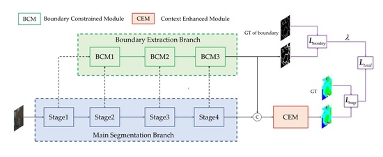
The overall structure of the high-resolution boundary-constrained and context-enhanced network (HBCNet) is shown in Figure 1.
The network consists of three parts: the image branch, the boundary branch and the context-enhanced module. The image branch takes HRNet, which includes four stages, as the baseline for feature extraction. Each stage connects the multi-resolution feature maps in parallel and repeatedly exchanges information on the sub-network for multi-scale fusion. The boundary branch is cascaded by three boundary-constrained modules. The first BCM inputs are the highest resolution feature maps of stage 1 and stage 2 in the baseline, and the next two BCM inputs come from the previous BCM and the corresponding baseline stage output. The last BCM not only outputs the results of boundary extraction, but also transfers them to the context-enhanced module (CEM). The CEM also consists of three portions: contextual feature expression (CFE), semantic attention extraction (SAE) and contextual enhancement representation (CER). First, the deep network features and the boundary representation are concatenated as input and the feature vectors of the different categories are obtained. Then, the previous outcome is handled with a self-attention mechanism and the feature expression combined with semantic information is extracted. Finally, the contextual enhancement representation is generated by integrating the semantic feature expression and the deep network features.

3.2. Boundary-Constrained Module

The boundary-constrained module is the critical part of the whole boundary branch. As shown in Figure 2, there are two inputs to this module: the first is a highest resolution feature map inside the stage of the baseline, the other is the previous BCM output.
Given a high-resolution input feature map X 1 R C 1 × H × W , we extract the dependencies of the internal channels of the feature maps through the global average pooling and obtain the result U . The channel c in U could be formalized as
U c = F g a p X 1 = 1 H × W i = 1 H j = 1 W X c i , j
Next, two full-connection layers are used for adaptive calibration so that the network can learn the interaction between each channel. The first connection layer is composed of a linear layer and a ReLU function, and the second is composed of a linear layer and a sigmoid function. The related process can be written as
Z = F e U , L = σ L 2 δ L 1 U
Here, σ denotes sigmoid function, δ denotes ReLU function, L 1 means linear layer R C 1 R C 1 r , L 2 means linear layer R C 1 r R C 2 , and r is the compression factor, which is used to reduce the amount of calculation with a default setting of 4.
After passing through the full-connection layers, we obtain the corresponding global feature expression Z and then utilize it to perform pointwise multiplication with the previous BCM output X 2 R C 2 × H × W and obtain high-resolution representations. Finally, we concatenate the initial input feature map with the high-resolution representations and gain the BCM output Y . The whole process can be defined as
Y = ( X 2 σ L 2 δ L 1 F g a p X 1 ) X 2
where denotes matrix pointwise operation, denotes concatenation of channels.
The BCM makes full use of the high-resolution feature representation of HRNet. The high-resolution feature maps have richer boundary and texture information, and the receptive field gradually increases with the continuous convolution operations. If we want to supervise the network training with boundary information, it is practical to do the extraction in high-resolution feature maps.

3.3. Context-Enhanced Module

The context-enhanced module (CEM) is designed with a self-attention mechanism and comprises many mathematical operations. As shown in Figure 3, the CEM is composed of three portions as follows: contextual feature representation (CFR), semantic attention extraction (SAE) and contextual enhancement representation (CER).
  • Contextual Feature Representation
First, the module input is processed with 1 × 1 Conv of quantity K and reshaped as X R K × H · W . Simultaneously the module input is also managed with 1 × 1 Conv of quantity C (equal to the total number of categories) and the distribution map ω R H · W × C is obtained by matrix reshape and transpose operation. Then the above outputs are handled with matrix multiplication, and we denote the result as contextual feature representation Y R K × C . The mth category feature vector Y m R K can be formalized as
Y m = F i = 1 H × W w i m X i
where the X i R K 1 m H · W means the feature vector of the ith pixel in X , w i m 1 m C is the relation between the ith pixel and the mth category, F denotes the transfer function, and H and W are the length and width of the feature map.
2.
Semantic Attention Extraction
Similar to [41,42], we adopt self-attention to perform semantic attention extraction. The Query matrix is calculated from the deep feature maps of the network and reshaped as Q R K × H · W , in which the corresponding feature expression vector size of each pixel is also K. The Key matrix K R K × C and the Value matrix V R C × K are further generated by 1 × 1 Conv-BN-ReLU with contextual feature representation that is derived from the previous step. While calculating the attention weight of a single pixel between different categories, we also use the softmax function to do the normalization. The related process can be written as
α i j = s o f t m a x Q T K d = e 1 d q i T k j j = 1 c e 1 d q i T k j
Here, q i denotes the Query vector of the ith pixel 1 i H · W , k j denotes the Key vector of the jth category 1 j C , and α R H · W × C means the semantic attention weight matrix. Then we utilize α to do matrix multiplication with the Value matrix, which aims to add weights on the Value vector of different categories and obtain the semantic attention extraction Z R H · W × K . The corresponding formula is
Z = j = 1 c α i j v j
where v j denotes the Value vector of the jth category 1 j C .
3.
Contextual Enhancement Representation
After gaining the semantic attention extraction, we concatenate it with the deep network feature, which comes from the initial module input to better train our network. The process can be defined as
Y = δ f σ f X Z
Here, both σ and δ denote BN-ReLU operation, f denotes 1 × 1 Conv, and denotes concatenation of channels.

3.4. Multi-Loss Function

As mentioned above, the boundary segmentation result originates from the boundary branch and calculates the corresponding boundary loss with the boundary ground truth. Meanwhile, the boundary ground truth is extracted from the image ground truth by Sobel operator. The specific process is as follows: First, the original image ground truth is processed by Sobel operators, and the gradient images corresponding X direction and Y direction are obtained, respectively. Then these two gradient images are weighted and merged into the overall gradient image. The final boundary ground truth is gained after the binarization of the overall gradient image.
We adopt a binary cross-entropy function to compute the boundary loss. The related formula can be written as
L b o u n d a r y = i = 1 H j = 1 W y i j l o g p i j + 1 y i j l o g 1 p i j
where y is the one-hot vector and y i j 0 , 1 , y i j = 1 means that the pixel i , j is the boundary pixel. p denotes the probability distribution of pixels classified as boundary in the image, and p i j represents the probability that pixel i , j is a boundary pixel.
The original image segmentation loss is calculated by the multi-classification cross-entropy function and can be defined as
L i m a g e = i = 1 H j = 1 W y i j l o g e p c k = 1 C e p k
Here, y is the one-hot vector and y i j 0 , 1 . y i j = 1 means that the pixel i , j belongs to the cth category. p denotes the probability distribution of the pixel i , j and p c represents the probability that pixel i , j belongs to the cth category. C denotes the number of categories.
The total loss is obtained by adding the image loss L i m a g e and the boundary loss L b o u n d a r y which is weighted by the factor λ . The related formula is as follows
L t o t a l = L i m a g e + λ L b o u n d a r y
The default setting of λ is 0.2.

4. Experiment

In this section, the datasets are first introduced and then the experiment settings and the evaluation metrics are elaborated. Finally, the experimental results for the ISPRS Vahingen and Potsdam benchmarks are analyzed.

4.1. Datasets

We performed experiments on the ISPRS 2D semantic benchmark datasets, including the Vahingen dataset and the Potsdam dataset [43]. Both datasets are typical and are always used as the benchmark datasets in remote sensing image segmentation. They consist of six ground categories with different labeled color, including impervious surfaces (white), building (blue), low vegetation (cyan), tree (green), car (yellow), and cluster (red). Figure 4 shows the overall view of the two datasets.
Potsdam: There are 38 high-resolution images of dimensions 6000 × 6000 with 5 cm ground sampling distance (GSD). Each image has three data formats, including IRRG, RGB, RGBIR—we only employ the IRRG images. Each image also has the corresponding ground truth and digital surface model (DSM)—we only use the ground truth. The same as the ISPRS 2-D semantic labeling contest, we use 24 images for training and validation—the remaining 14 images are only used for testing. Considering the limitation in GPU memory, we crop the image to slices with a size of 512 × 512 pixels, each slice overlapped with 256 × 256 pixels. The ratio of the training set to the validating set is 4 : 1 . Finally, we obtain 10,156 slices for training, 2540 slices for validation, and 7406 slices for testing.
Vahingen: There are 33 high-resolution images with 9 cm ground sampling distance of sizes ranging from 1996 × 1995 to 3816 × 2550 . All the images are in IRRG data format with the corresponding ground truth and DSM. The same as the ISPRS 2D semantic labeling contest, we employ 16 images for training and validation—the remaining 17 images are kept only for testing. We crop the image to slices of size 256 × 256 , each slice overlapped with 128 × 128 pixels. The ratio between the training set and the validation set is also 4 : 1 . In the end, we obtain 3540 slices for training, 886 slices for validation and 5074 slices for testing.
We apply the ground truth with eroded boundaries to evaluate the model performance.

4.2. Experiment Settings and Evaluation Metrics

The HBCNet was constructed under the PyTorch deep-learning framework with a Pycharm compiler and used the pretrained HRNet_w48 as the network baseline. All the experiments were conducted on a single NVIDIA RTX 3090 GPU (24 GB RAM). The stochastic gradient descent with momentum (SGDM) optimizer was set to guide the optimization. The initial learning rate was 0.005 and the momentum was 0.9. A poly learning rate policy was adopted to adjust the learning rate during the network training. The batch size was 8 and the total number of training epochs was 200. In terms of data augmentation, we only employed random vertical and horizontal flip, and random rotation with specified angles 0   90 °   180 °   270 ° . In addition, we applied the test-time augmentation (TTA) method during the inference process, which included multi-scale input and transpose operations. All the settings are detailed in Table 1.
The evaluation metrics to measure the performance on the two datasets were the same, including overall accuracy (OA), F1 score, m-F1 (mean F1 score), intersection over union (IoU), mean intersection over union (mIoU), precision (P), and recall (R). The corresponding calculation formulas are as follows
OA = k = 1 N T P k k = 1 N T P k + F N k P k = T P k T P k + F P k R k = T P k T P k + F N k F 1 k = 2 × P k × R k P k + R k m F 1 = 1 N k = 1 N F 1 k I o U k = T P k T P k + F P k + F N k m I o U = 1 N k = 1 N I O U k
Here, TP, TN, FP, FN denote true positive, true negative, false positive and false negative number of pixels, respectively, in the confusion matrix. Figure 5 shows the variation in the evaluation metrics (m-F1, OA, mIoU) and loss during the training phase with 200 epochs for the Potsdam validation dataset.

4.3. Experiment Results

4.3.1. Results for the Vahingen Dataset

Table 2 shows the experimental results for HBCNet and other models in the published paper for the Vahingen dataset. The results of some methods can be found on the official website of ISPRS 2D semantic labeling contest [44], including UFMG_4 [45], CVEO [17], CASIA2 [46] and HUSTW [47]. Based on the original paper, we selected the dilated ResNet-101 [48] as the baseline to train some networks, which consisted of FCN [49], UNet [4], EncNet [33], PSPNet [8], DANet [35] and Deeplabv3+ [11]. The corresponding super parameters and image size used in network training were the same as for HBCNet. In Table 1, the values in bold are the best and the values underlined are the second best. It is obvious that the HBCNet far outperformed the other models, achieving the highest m-F1 of 91.32%, OA of 91.72% and mIoU of 84.21%. An improvement of 0.72% in mIoU and of 0.36% in m-F1 compared with the second-best methods was observed. The F1-score for building was also the highest among the ground categories. Figure 6 demonstrates qualitatively the partial inference results of HBCNet and other models on the test dataset.
FCN had a good segmentation effect on large-scale objects, such as buildings, but it was not sensitive to details, and there were many noise points. UNet adopted the skip connection to integrate the shallow and the deep feature information, making up for the loss of details to some extent. Compared with the two models above, Deeplabv3+ and DANet achieved better effects. The former obtained a larger receptive field through atrous spatial pyramid pooling, and the latter employed channel and spatial attention mechanisms to capture more context feature information. However, it is clear from Figure 6 that some buildings and trees had shadows and were intertwined with impervious surfaces, and that the above models often generated errors when dealing with such cases. HBCNet introduced boundary information for supervision in the training process and achieved the best result. While learning ground feature information, it also combined image boundary features for feedback and then enhanced the model anti-interference capability to shadows and other external factors.

4.3.2. Results for the Potsdam Dataset

Table 3 displays the results for HBCNet and the other networks for the Potsdam dataset. Related results for UFMG_4 [45], CVEO [17], CASIA2 [46] and HUSTW [47] can be found on the official website [50]. It was evident that HBCNet produced positive results. The evaluation metrics for m-F1 and mIoU surpassed those of the other methods. There was a 0.53 % improvement in mIoU and a 0.18 % improvement in m-F1 compared with the second-best methods. Moreover, the F1-scores of HBCNet for impervious surfaces, tree and car were also the best.
Figure 7 presents a comparison of partial inference results for HBCNet and the other models. Compared to the original images, the trees and grassland are staggered and the ground color is close to that of the grassland. During the actual segmentation process, UNet and other models often produce errors and the boundary accuracy among different ground categories needs to be reinforced. HBCNet not only introduces boundary information, but also enhances the semantic correlation between pixels of the same category with the context-enhanced module. The contextual representation of the same category has been advanced and has alleviated the problem of high intra-class variance and low inter-class variance.

5. Discussion

In this section, we consider the ablation study on the Vahingen and Potsdam datasets in detail to validate the effects of the corresponding modules. We also explore the huge benefit of the test-time augmentation (TTA) method. Finally, we discuss the limitations of our model and future research directions.

5.1. Ablation Study

To avoid the TTA method interfering with the ablation experimental results, we did not adopt it in the ablation study. The comparison of the functions with different modules included four combinations: the original baseline, adding the boundary-constrained module only, adding the contextual enhanced module only, and adding both modules. The evaluation metrics still employed m-F1, OA and mIoU.
Table 4 shows the effects of the two modules for the Vahingen dataset. Compared to not adding any module, adding BCM and CEM advanced the accuracy to some extent. BCM achieved an approximately 0.24% improvement in m-F1 and a 0.37% improvement in mIoU. CEM yielded 0.1% and 0.14% improvement for m-F1 and mIoU. After integrating both BCM and CEM, there were further enhancements. The HBCNet combining BCM and CEM together obtained the highest m-F1 of 90.44%, an mIoU of 82.76% and OA of 90.82%. The m-F1 and mIoU increased significantly, with nearly 0.38% and 0.59% improvement, respectively.
Table 5 shows the ablation experimental results for the Potsdam dataset. In comparison with the original baseline, both BCM and CEM resulted in improvements. BCM resulted in a 0.15% improvement in m-F1, a 0.27% improvement in mIoU and a 0.17% improvement in OA. CEM resulted in approximately 0.2%, 0.35% and 0.24% increases in m-F1, mIoU and OA, respectively. Incorporating both BCM and CEM, HBCNet also resulted in significant improvements, with the best m-F1 results of 92.86%, mIoU of 86.92% and OA of 91.39%.
The following figures are qualitative results for the ablation study on the Potsdam test dataset. Figure 8 shows comparisons of partial segmentation results between the baseline and HBCNet. The grass and ground are interweaved and the color of some building surfaces are similar to the low vegetation. The baseline produced segmentation errors while handling the above cases, but HBCNet, by integrating boundary information and contextual features, can achieve good performance. Figure 9 shows the visual feature maps of the last BCM output. It is evident that the boundary information in the original images is effectively extracted by the boundary branch. Figure 10 displays the predictions of baseline and the predictions of baseline with CEM. In the results of baseline, the grassland and ground, and grassland and building are easily confused. After adding the CEM, the results were effectively improved, as CEM introduced contextual representations and enhanced the semantic correlation between pixels of the same category.
We also employed the method of test-time enhancement (TTA) to reinforce the model performance. The main process of TTA is as follows: Firstly, creating multiple inputs with the same original image, such as clipping with different regions and zooming with different scales; then inputting all the images into the model which has been trained well and obtaining the corresponding outputs; finally, conducting the inverse transformation and obtaining the average segmentation result of multiple outputs. In the actual process, we adopted the two methods of TTA: multi-scale inputs with four image scales 0.5 ,   0.75 ,   1 ,   1.5 and various transpose operations. Table 6 and Table 7 demonstrate the results for the Vahingen and Potsdam datasets.
As is shown in Table 6 and Table 7, both multi-scale inputs and transpose operations can significantly improve the segmentation accuracy. It is possible that our model has the capacity for multi-scale feature extraction. Large-scale ground objects, such as buildings and impervious surfaces, can be segmented better on smaller resolution feature maps, while small-scale ground objects, such as cars, need more detail and therefore the prediction results on the higher feature maps may be better. We integrated the above characteristics through multi-scale inputs and transpose operations to achieve acceptable improvements.

5.2. Limitations and Future Research Directions

In addition to the metrics (e.g., OA, F1-score and mIoU) to evaluate the segmentation results, model complexity often needs to be considered. The most common indicators of model complexity are floating point operations per second (FLOPs), and the number of model parameters (Params). Table 8 displays the comparisons of model complexity between HBCNet and other models. The calculation of FLOPs is affected by the size of the input image; this was set to 256 × 256.
As shown in Table 8, the FLOPs of HBCNet were the lowest compared to the other models, which implies a faster inference speed. However, HBCNet has relatively more parameters and occupies more memory, which is an obvious deficiency of our network at present. Our model is also still limited by the labels of datasets. Both image loss and boundary loss need to be calculated in combination with the image ground truth. It is still a typical fully supervised network. In the future, we intend to integrate the generative adversarial network (GANs) [51] to reduce reliance on dataset labels and to obtain high segmentation accuracy.

6. Conclusions

In this paper, we propose the high-resolution boundary-constrained and context-enhanced network (HBCNet) for remote sensing image segmentation. Considering the problems of ground objects blocked by shadow, higher intra-class variance and lower inter-class variance, we designed a boundary-constrained module and a context-enhanced module. The boundary-constrained module is embedded into the main segmentation network to form a parallel branch extraction branch, which not only outputs the boundary segmentation results but also supervises the network training. The context-enhanced module introduces contextual representations and enhances the semantic correlation among pixels of the same category with the self-attention mechanism. We conducted experiments using the ISPRS 2D semantic benchmark Vahingen and Potsdam datasets and obtained excellent results. The m-F1 of HBCNet for the two datasets were 91.31% and 93.38%, respectively, surpassing that for existing CNN-based methods. In the future, we will undertake further research to ensure our model is lightweight and to reduce dependence on dataset labels.

Author Contributions

Y.X. and J.J. conceived the idea; Y.X. designed the network and performed the experiments; Y.X. and J.J. analyzed the results; Y.X. wrote the paper; J.J. offered comments and supervised the paper. All authors have read and agreed to the published version of the manuscript.

Funding

This research was supported by the National Natural Science Foundation of China (NSFC) under grant number 61725501.

Data Availability Statement

No new data were created or analyzed in this paper. Data sharing is not applicable to this article.

Acknowledgments

This work was supported by the Key Laboratory of Precision Opto-mechatronics Technology, Ministry of Education, Beihang University, China. The authors would like to thank ISPRS for providing the 2D semantic labeling contest datasets and results.

Conflicts of Interest

The authors declare no conflict of interest.

Abbreviations

The following abbreviations are employed in this manuscript.
CNNConvolutional Neural Network
PPMPyramid Pooling Module
ASPPAtrous Spatial Pyramid Pooling
DSMDigital Surface Model
HBCNetHigh-resolution Boundary-constrained and Context-enhanced Network
BCMBoundary-constrained Module
CEMContext-enhanced Module
TTATest-Time Augmentation
ISPRSInternational Society for Photogrammetry and Remote Sensing
GSDGround Sampling Distance
SGDMStochastic Gradient Descent with Momentum
GPUGraphics Processing Unit
IDEIntegrated Development Environment
LRLearning Rate
OAOverall Accuracy
m-F1Mean F1-score
IoUIntersection Over Union
mIoUMean Intersection Over Union
FLOPsFloating Point Operations Per Second
ParamsParameters

References

  1. Zhang, Q.; Seto, K.C. Mapping urbanization dynamics at regional and global scales using multi-temporal DMSP/OLS nighttime light data. Remote Sens. Environ. 2011, 115, 2320–2329. [Google Scholar] [CrossRef]
  2. Matikainen, L.; Karila, K. Segment-based land cover mapping of a suburban area—Comparison of high-resolution remotely sensed datasets using classification trees and test field points. Remote Sens. 2011, 3, 1777–1804. [Google Scholar] [CrossRef] [Green Version]
  3. Moser, G.; Serpico, S.B.; Benediktsson, J.A. Land-cover mapping by Markov modeling of spatial–contextual information in very-high-resolution remote sensing images. Proc. IEEE 2012, 101, 631–651. [Google Scholar] [CrossRef]
  4. Ronneberger, O.; Fischer, P.; Brox, T. U-net: Convolutional networks for biomedical image segmentation. In Proceedings of the International Conference on Medical Image Computing and Computer-Assisted Intervention, Munich, Germany, 5–9 October 2015; pp. 234–241. [Google Scholar]
  5. Badrinarayanan, V.; Kendall, A.; Cipolla, R. Segnet: A deep convolutional encoder-decoder architecture for image segmentation. Pattern Anal. Mach. Intell. 2017, 39, 2481–2495. [Google Scholar] [CrossRef] [PubMed]
  6. Lin, G.; Milan, A.; Shen, C.; Reid, I. Refinenet: Multi-path refinement networks for high-resolution semantic segmentation. In Proceedings of the IEEE Conference on Computer Vision and Pattern Recognition, Honolulu, HI, USA, 21–26 July 2017; pp. 1925–1934. [Google Scholar]
  7. He, K.; Zhang, X.; Ren, S.; Sun, J. Deep residual learning for image recognition. In Proceedings of the IEEE Conference on Computer Vision and Pattern Recognition, Las Vegas, NV, USA, 26 June–1 July 2016; pp. 770–778. [Google Scholar]
  8. Zhao, H.; Shi, J.; Qi, X.; Wang, X.; Jia, J. Pyramid scene parsing network. In Proceedings of the IEEE Conference on Computer Vision and Pattern Recognition, Honolulu, HI, USA, 21–26 July 2017; pp. 2881–2890. [Google Scholar]
  9. Chen, L.-C.; Papandreou, G.; Kokkinos, I.; Murphy, K.; Yuille, A.L. Deeplab: Semantic image segmentation with deep convolutional nets, atrous convolution, and fully connected crfs. IEEE Trans. Pattern Anal. Mach. Intell. 2017, 40, 834–848. [Google Scholar] [CrossRef] [Green Version]
  10. Chen, L.-C.; Papandreou, G.; Kokkinos, I.; Murphy, K.; Yuille, A.L. Semantic image segmentation with deep convolutional nets and fully connected crfs. arXiv 2014, arXiv:1412.7062. [Google Scholar]
  11. Chen, L.-C.; Zhu, Y.; Papandreou, G.; Schroff, F.; Adam, H. Encoder-decoder with atrous separable convolution for semantic image segmentation. In Proceedings of the European Conference on Computer Vision (ECCV), Munich, Germany, 8–14 September 2018; pp. 801–818. [Google Scholar]
  12. Sun, K.; Xiao, B.; Liu, D.; Wang, J. Deep high-resolution representation learning for human pose estimation. In Proceedings of the IEEE/CVF Conference on Computer Vision and Pattern Recognition, Long Beach, CA, USA, 15–20 June 2019; pp. 5693–5703. [Google Scholar]
  13. Sun, K.; Zhao, Y.; Jiang, B.; Cheng, T.; Xiao, B.; Liu, D.; Mu, Y.; Wang, X.; Liu, W.; Wang, J. High-resolution representations for labeling pixels and regions. arXiv 2019, arXiv:1904.04514. [Google Scholar]
  14. Chaurasia, A.; Culurciello, E. Linknet: Exploiting encoder representations for efficient semantic segmentation. In Proceedings of the 2017 IEEE Visual Communications and Image Processing (VCIP), St. Petersburg, FL, USA, 10–13 December 2017; pp. 1–4. [Google Scholar]
  15. Yu, C.; Wang, J.; Peng, C.; Gao, C.; Yu, G.; Sang, N. Bisenet: Bilateral segmentation network for real-time semantic segmentation. In Proceedings of the European Conference on Computer Vision (ECCV), Munich, Germany, 8–14 September 2018; pp. 325–341. [Google Scholar]
  16. Li, H.; Xiong, P.; Fan, H.; Sun, J. Dfanet: Deep feature aggregation for real-time semantic segmentation. In Proceedings of the IEEE/CVF Conference on Computer Vision and Pattern Recognition, Long Beach, CA, USA, 15–20 June 2019; pp. 9522–9531. [Google Scholar]
  17. Chen, G.; Zhang, X.; Wang, Q.; Dai, F.; Gong, Y.; Zhu, K. Symmetrical dense-shortcut deep fully convolutional networks for semantic segmentation of very-high-resolution remote sensing images. IEEE J. Sel. Top. Appl. Earth Obs. Remote Sens. 2018, 11, 1633–1644. [Google Scholar] [CrossRef]
  18. Yue, K.; Yang, L.; Li, R.; Hu, W.; Zhang, F.; Li, W. TreeUNet: Adaptive Tree convolutional neural networks for subdecimeter aerial image segmentation. ISPRS J. Photogramm. Remote Sens. 2019, 156, 1–13. [Google Scholar] [CrossRef]
  19. Xie, S.; Girshick, R.; Dollár, P.; Tu, Z.; He, K. Aggregated residual transformations for deep neural networks. In Proceedings of the IEEE Conference on Computer Vision and Pattern Recognition, Honolulu, HI, USA, 21–26 July 2017; pp. 1492–1500. [Google Scholar]
  20. Yu, B.; Yang, L.; Chen, F. Semantic segmentation for high spatial resolution remote sensing images based on convolution neural network and pyramid pooling module. IEEE J. Sel. Top. Appl. Earth Obs. Remote Sens. 2018, 11, 3252–3261. [Google Scholar] [CrossRef]
  21. Ding, L.; Zhang, J.; Bruzzone, L. Semantic Segmentation of Large-Size VHR Remote Sensing Images Using a Two-Stage Multiscale Training Architecture. IEEE Trans. Geosci. Remote Sens. 2020, 58, 5367–5376. [Google Scholar] [CrossRef]
  22. Gao, X.; Sun, X.; Yan, M.; Sun, H.; Fu, K.; Zhang, Y.; Ge, Z. Road extraction from remote sensing images by multiple feature pyramid network. In Proceedings of the IGARSS 2018–2018 IEEE International Geoscience and Remote Sensing Symposium, Valencia, Spain, 22–27 July 2018; pp. 6907–6910. [Google Scholar]
  23. Shang, R.H.; Zhang, J.Y.; Jiao, L.C.; Li, Y.Y.; Marturi, N.; Stolkin, R. Multi-scale Adaptive Feature Fusion Network for Semantic Segmentation in Remote Sensing Images. Remote Sens. 2020, 12, 872. [Google Scholar] [CrossRef] [Green Version]
  24. Kaiser, P.; Wegner, J.D.; Lucchi, A.; Jaggi, M.; Hofmann, T.; Schindler, K. Learning aerial image segmentation from online maps. IEEE Trans. Geosci. Remote Sens. 2017, 55, 6054–6068. [Google Scholar] [CrossRef]
  25. Audebert, N.; le Saux, B.; Lefèvre, S. Joint learning from earth observation and openstreetmap data to get faster better semantic maps. In Proceedings of the IEEE Conference on Computer Vision and Pattern Recognition Workshops, Honolulu, HI, USA, 21–26 July 2017; pp. 67–75. [Google Scholar]
  26. Cao, Z.; Fu, K.; Lu, X.; Diao, W.; Sun, H.; Yan, M.; Yu, H.; Sun, X. End-to-end DSM fusion networks for semantic segmentation in high-resolution aerial images. IEEE Geosci. Remote Sens. Lett. 2019, 16, 1766–1770. [Google Scholar] [CrossRef]
  27. Zheng, X.; Wu, X.; Huan, L.; He, W.; Zhang, H. A Gather-to-Guide Network for Remote Sensing Semantic Segmentation of RGB and Auxiliary Image. IEEE Trans. Geosci. Remote Sens. 2021, 60, 1–15. [Google Scholar] [CrossRef]
  28. Liu, S.; Ding, W.R.; Liu, C.H.; Liu, Y.; Wang, Y.F.; Li, H.G. ERN: Edge Loss Reinforced Semantic Segmentation Network for Remote Sensing Images. Remote Sens. 2018, 10, 1339. [Google Scholar] [CrossRef] [Green Version]
  29. Li, A.; Jiao, L.; Zhu, H.; Li, L.; Liu, F. Multitask Semantic Boundary Awareness Network for Remote Sensing Image Segmentation. IEEE Trans. Geosci. Remote Sens. 2021, 60, 1–15. [Google Scholar] [CrossRef]
  30. Xu, Z.; Zhang, W.; Zhang, T.; Li, J. HRCNet: High-Resolution Context Extraction Network for Semantic Segmentation of Remote Sensing Images. Remote Sens. 2021, 13, 71. [Google Scholar] [CrossRef]
  31. Xu, Z.; Zhang, W.; Zhang, T.; Yang, Z.; Li, J. Efficient Transformer for Remote Sensing Image Segmentation. Remote Sens. 2021, 13, 3585. [Google Scholar] [CrossRef]
  32. Hu, J.; Shen, L.; Sun, G. Squeeze-and-excitation networks. In Proceedings of the IEEE Conference on Computer Vision and Pattern Recognition, Salt Lake City, UT, USA, 18–23 June 2018; pp. 7132–7141. [Google Scholar]
  33. Zhang, H.; Dana, K.; Shi, J.; Zhang, Z.; Wang, X.; Tyagi, A.; Agrawal, A. Context encoding for semantic segmentation. In Proceedings of the IEEE Conference on Computer Vision and Pattern Recognition, Salt Lake City, UT, USA, 18–23 June 2018; pp. 7151–7160. [Google Scholar]
  34. Zhao, H.; Zhang, Y.; Liu, S.; Shi, J.; Loy, C.C.; Lin, D.; Jia, J. Psanet: Point-wise spatial attention network for scene parsing. In Proceedings of the European Conference on Computer Vision (ECCV), Munich, Germany, 8–14 September 2018; pp. 267–283. [Google Scholar]
  35. Fu, J.; Liu, J.; Tian, H.; Li, Y.; Bao, Y.; Fang, Z.; Lu, H. Dual attention network for scene segmentation. In Proceedings of the IEEE/CVF Conference on Computer Vision and Pattern Recognition, Long Beach, CA, USA, 15–20 June 2019; pp. 3146–3154. [Google Scholar]
  36. Huang, Z.; Wang, X.; Huang, L.; Huang, C.; Wei, Y.; Liu, W. Ccnet: Criss-cross attention for semantic segmentation. In Proceedings of the IEEE/CVF International Conference on Computer Vision, Long Beach, CA, USA, 15–20 June 2019; pp. 603–612. [Google Scholar]
  37. Li, X.; Zhong, Z.; Wu, J.; Yang, Y.; Lin, Z.; Liu, H. Expectation-maximization attention networks for semantic segmentation. In Proceedings of the IEEE/CVF International Conference on Computer Vision, Long Beach, CA, USA, 15–20 June 2019; pp. 9167–9176. [Google Scholar]
  38. Niu, R.; Sun, X.; Tian, Y.; Diao, W.; Chen, K.; Fu, K. Hybrid multiple attention network for semantic segmentation in aerial images. IEEE Trans. Geosci. Remote Sens. 2021, 60, 1–18. [Google Scholar] [CrossRef]
  39. Ding, L.; Tang, H.; Bruzzone, L. LANet: Local attention embedding to improve the semantic segmentation of remote sensing images. IEEE Trans. Geosci. Remote Sens. 2020, 59, 426–435. [Google Scholar] [CrossRef]
  40. Liu, R.; Mi, L.; Chen, Z. AFNet: Adaptive Fusion Network for Remote Sensing Image Semantic Segmentation. IEEE Trans. Geosci. Remote Sens. 2020, 59, 7871–7886. [Google Scholar] [CrossRef]
  41. Yuan, Y.; Chen, X.; Chen, X.; Wang, J. Object-contextual representations for semantic segmentation. In Proceedings of the European Conference on Computer Vision (ECCV), Glasgow, UK, 23-28 August 2020; pp. 173–190. [Google Scholar]
  42. Vaswani, A.; Shazeer, N.; Parmar, N.; Uszkoreit, J.; Jones, L.; Gomez, A.N.; Kaiser, Ł.; Polosukhin, I. Attention is all you need. In Proceedings of the Advances in Neural Information Processing Systems, Long Beach, CA, USA, 4–9 December 2017; pp. 5998–6008. [Google Scholar]
  43. ISPRS 2D Semantic Labeling Contest. Available online: https://www.isprs.org/education/benchmarks/UrbanSemLab/semantic-labeling.aspx (accessed on 1 March 2022).
  44. ISPRS 2D Semantic Labeling Contest Results in Vahingen Dataset. Available online: https://www.isprs.org/education/benchmarks/UrbanSemLab/results/vaihingen-2d-semantic-labeling.aspx (accessed on 1 March 2022).
  45. Nogueira, K.; Dalla Mura, M.; Chanussot, J.; Schwartz, W.R.; dos Santos, J.A. Dynamic multicontext segmentation of remote sensing images based on convolutional networks. IEEE Trans. Geosci. Remote Sens. 2019, 57, 7503–7520. [Google Scholar] [CrossRef] [Green Version]
  46. Liu, Y.; Fan, B.; Wang, L.; Bai, J.; Xiang, S.; Pan, C. Semantic labeling in very high resolution images via a self-cascaded convolutional neural network. ISPRS J. Photogramm. Remote Sens. 2018, 145, 78–95. [Google Scholar] [CrossRef] [Green Version]
  47. Sun, Y.; Tian, Y.; Xu, Y. Problems of encoder-decoder frameworks for high-resolution remote sensing image segmentation: Structural stereotype and insufficient learning. Neurocomputing 2019, 330, 297–304. [Google Scholar] [CrossRef]
  48. Dilated ResNet-101 as Baseline for Models of Semantic Segmentation. Available online: https://github.com/Tramac/awesome-semantic-segmentation-pytorch (accessed on 1 March 2022).
  49. Long, J.; Shelhamer, E.; Darrell, T. Fully convolutional networks for semantic segmentation. In Proceedings of the IEEE Conference on Computer Vision and Pattern Recognition, Boston, MA, USA, 7–12 June 2015; pp. 3431–3440. [Google Scholar]
  50. ISPRS 2D Semantic Labeling Contest Results in Potsdam Dataset. Available online: https://www.isprs.org/education/benchmarks/UrbanSemLab/results/potsdam-2d-semantic-labeling.aspx (accessed on 1 March 2022).
  51. Goodfellow, I.J.; Pouget-Abadie, J.; Mirza, M.; Xu, B.; Warde-Farley, D.; Ozair, S.; Courville, A.; Bengio, Y. Generative adversarial networks. arXiv 2014, arXiv:1406.2661. [Google Scholar] [CrossRef]
Figure 1. The overall structure of our network.
Remotesensing 14 01859 g001
Figure 2. The detailed framework of boundary-constrained module.
Remotesensing 14 01859 g002
Figure 3. The elaborate structure of the context-enhanced module.
Remotesensing 14 01859 g003
Figure 4. The overall view of ISPRS 2D semantic benchmark datasets. (From left to right) Columns show the images of the Potsdam dataset and images of the Vahingen dataset.
Remotesensing 14 01859 g004
Figure 5. The variation in evaluation metrics and loss during the training phase with 200 epochs for the Potsdam validation dataset. (From left to right) Columns reveal the process of OA, m-F1, mIoU changing with epochs, and the process of loss changing with epochs.
Remotesensing 14 01859 g005
Figure 6. Qualitative comparisons between our method and other models for the Vahingen test dataset. (From left to right) Columns demonstrate the original images, the image ground truth, the predictions of FCN, UNet, DANet, Deeplabv3+ and the predictions of our method.
Remotesensing 14 01859 g006
Figure 7. Qualitative comparisons between our method and other models for the Potsdam test dataset. (From left to right) Columns demonstrate the original images, the image ground truth, the predictions of FCN, UNet, DANet, Deeplabv3+, and the predictions of HBCNet.
Remotesensing 14 01859 g007
Figure 8. Qualitative comparisons between the baseline and our method. (From left to right) Columns show the original images, the image ground truth, the predictions of baseline and the predictions of HBCNet.
Remotesensing 14 01859 g008
Figure 9. Visualizations of output features from the last BCM. (From left to right) Columns show the original images, the image ground truth, the boundary ground truth and the output features of the last BCM.
Remotesensing 14 01859 g009
Figure 10. Qualitative comparisons between the baseline and the baseline with CEM. (From left to right) Columns display the original images, the image ground truth, the predictions of baseline and the predictions of the baseline with CEM.
Remotesensing 14 01859 g010
Table 1. Experimental settings.
ConfigurationContents
Operating systemUbuntu 18.04.5 LTS
Deep-learning frameworkPytorch 1.7.1 and Torchvision 0.8.2
GPUNVIDIA RTX 3090 GPU (24 GB RAM)
Parallel computer platformCuda 11.0 and Cudnn 8.0.5
ProgramPython 3.8.5
IDEPycharm 2020.2.5
BaselineHRNet_w48
OptimizerSGDM
Learning rate0.005
LR policyPoly
Batch size8
Total epochs200
Momentum0.9
Data augmentationRandom flip and Random rotate
Loss functionCrossEntropy
Table 2. Experimental results (%) for the Vahingen dataset. The values in bold are the best and the values underlined are the second best.
MethodImp. Surf.BuildingLow Veg.TreeCarm-F1OAmIoU
CVEO [17]90.5092.4081.7088.5079.4086.5088.3076.63
UFMG_4 [45]91.1094.5082.9088.8081.3087.7289.4078.51
HUSTW [47]93.3096.1086.4090.8074.6088.2491.6079.99
FCN [49]91.2794.1681.8188.5286.5988.4789.1479.58
TreeUNet [18]92.5094.9083.6089.6085.9089.3090.40\
UNet [4]92.6695.2583.5289.3686.1689.3990.4181.08
EncNet [33]92.4995.3383.5689.2586.8289.4990.3881.23
PSPNet [8]92.5095.2483.4889.3187.0889.5290.3681.28
DANet [35]92.6095.2783.6089.4387.2889.6490.4481.46
Deeplabv3+ [11]92.8795.6084.3189.7487.9290.0990.8582.19
CASIA2 [46]93.2096.0084.7089.9086.7090.1091.1082.59
SBANet [29]94.3692.9183.4489.5891.4390.3490.59\
AFNet [40]93.4095.9086.0090.7087.2090.6091.6083.10
HMANet [38]93.5095.8685.4190.4089.6390.9691.4483.49
HRNet [13]92.7395.7483.7089.6188.5490.0690.7082.17
HBCNet93.6096.1385.9590.5390.4091.3291.7284.21
Table 3. Experimental results (%) for the Potsdam dataset. The values in bold are the best and the values underlined are the second best.
MethodImp. Surf.BuildingLow Veg.TreeCarm-F1OAmIoU
UFMG_4 [45]90.8095.6084.4084.3092.4089.5087.9081.61
CVEO [17]91.2094.5086.4087.4095.4090.9889.0083.75
FCN [49]92.0795.6686.2787.4495.7591.4489.6384.48
TreeUNet [18]93.1097.3086.8087.1095.8092.0090.70\
UNet [4]93.0396.7987.0188.0296.5392.2890.6385.94
EncNet [33]93.3496.8587.2188.2696.3592.4090.9286.14
CASIA2 [46]93.3097.0087.7088.4096.2092.5291.1086.49
PSPNet [8]93.2396.9187.7388.4696.3492.5391.0486.34
DANet [35]93.3797.0287.7388.4796.3092.5891.1586.42
HUSTW [47]93.6097.6088.5088.8094.6092.6291.6086.72
Deeplabv3+ [11]93.5597.2287.6588.5796.6992.7391.2086.71
SBANet [29]93.8398.0688.9789.4894.7193.0192.80\
AFNet [40]94.2097.2089.2089.4095.1093.0292.2087.10
HMANet [38]93.8597.5688.6589.1296.8493.2092.2187.28
HRNet [13]93.6697.1487.5188.4796.3392.6291.1586.51
HBCNet94.2997.5488.4989.5897.0093.3891.9787.81
Table 4. Ablation experimental results (%) for the Vahingen dataset. The values in bold are the best.
MethodBCMCEMm-F1mIoUOA
Baseline 90.0682.1790.70
Baseline + BCM 90.3082.5490.76
Baseline + CEM 90.1682.3190.70
Baseline + BCM + CEM(HBCNet)90.4482.7690.82
Table 5. Ablation experimental results (%) for the Potsdam dataset. The values in bold are the best.
MethodBCMCEMm-F1mIoUOA
Baseline 92.6286.5191.15
Baseline + BCM 92.7786.7891.32
Baseline + CEM 92.8286.8691.39
Baseline + BCM + CEM(HBCNet)92.8686.9291.39
Table 6. Results of different TTA methods for the Vahingen dataset. MS means multi-scale inputs and TS means transpose operations. The values in bold are the best.
MethodMSTSm-F1OAmIoU
HBCNet 90.4490.8282.76
HBCNet 91.1791.4783.97
HBCNet 91.2391.6484.06
HBCNet91.3291.7284.21
Table 7. Results of different TTA methods for the Potsdam dataset. MS means multi-scale inputs and TS means transpose operations. The values in bold are the best.
MethodMSTSm-F1OAmIoU
HBCNet 92.8691.3986.92
HBCNet 93.3491.9387.73
HBCNet 93.2891.8687.63
HBCNet93.3891.9787.81
Table 8. Comparisons of model complexity between HBCNet and other networks. The values in bold are the best.
MethodFLOPs (G)Params (M)
FCNs25.5218.64
UNet74.4128.05
PSPNet63.8265.58
DANet68.9366.43
Deeplabv3+62.1162.28
HBCNet24.1566.17
Publisher’s Note: MDPI stays neutral with regard to jurisdictional claims in published maps and institutional affiliations.

