Article

Multi-Sensor Analysis of Snow Seasonality and a Preliminary Assessment of SAR Backscatter Sensitivity to Arctic Vegetation: Limits and Capabilities

1
Department of Agriculture, Food, Environment, and Forestry (DAGRI), University of Florence, Piazzale Delle Cascine 18, 50144 Florence, Italy
2
Institute for Earth Observation, Eurac Research, 39100 Bolzano, Italy
3
Climatic Department, NORCE, Norwegian Research Centre AS, P.O. Box 6434, N-9294 Tromsø, Norway
4
Department of Arctic and Marine Biology, University of Tromsø, PO Box 6050, N-9037 Tromsø, Norway
5
Norwegian Institute for Nature Research (NINA), FRAM—High North Research Centre for Climate and the Environment, P.O. Box 6606, N-9296 Tromsø, Norway
*
Author to whom correspondence should be addressed.
Remote Sens. 2022, 14(8), 1866; https://doi.org/10.3390/rs14081866
Submission received: 26 February 2022 / Revised: 30 March 2022 / Accepted: 9 April 2022 / Published: 13 April 2022

Abstract

:
Snow melt timing and the last day of snow cover have a significant impact on vegetation phenology in the Svalbard archipelago. The aim of this study is to assess the seasonal variations of the snow using a multi-sensor approach and to analyze the sensitivity of the Synthetic Aperture Radar (SAR) backscatter to vegetation growth and soil moisture in an arctic environment. A combined approach using time series data from active remote sensing sensors such as SAR and passive optical sensors is a known technique in snow monitoring, while there is little knowledge of the radar C-band’s response pattern to vegetation dynamics in the arctic. First, we created multi-sensor masks using the HV backscatter coefficients from Sentinel-1 and the Normalized Difference Snow Index (NDSI) time series from Sentinel-2, monitoring the snow dynamics in Adventdalen (Svalbard) for the season from 2017 to 2018. Second, radar sensitivity analysis was performed using the HV polarized channel responses to vegetation growth and soil moisture dynamics. (1) Our results showed that the C-band radar data are capable of monitoring the seasonal variability in timing of snow melting in Adventdalen, revealing an earlier start by approximately 20 days in 2018 compared to 2017. (2) From the sensitivity analyses, the HV channel showed a major response to the vegetation component in areas with drier graminoid dominated vegetation without water-saturated soil (R = 0.69). However, the temperature was strongly correlated with the HV channel (R = 0.74) during the years with delayed snow melting. Areas of frozen tundra with drier vegetation dominated by graminoids had delayed soil thawing processes and therefore this may limit the ability of the radar to follow the vegetation growth pattern and soil moisture.

Graphical Abstract

1. Introduction

The timing of snow melt and the first day free of snow are considered indicators of Arctic climate and ecosystem status in response to global warming [1]. Moreover, the depth of snow and the period of snow melt contribute significantly to defining the phenological phases of vegetation [2,3] and plant biomass [4]. Due to an increase in winter precipitation [5], as well as in the frequency of extreme weather events in the Svalbard archipelago [6,7], snow cover monitoring is highly important.
Along with the ability to detect snow seasonality, there is a growing interest in studying the relationship between the timing of snow melt and vegetation phenology (late snow, onset of the growing season, and advanced snow melting). Malnes et al. (2016) [8] used satellite remote sensing (MODIS) over northern Norway in order to detect the snow covered season with significant accuracy due to start (r = 0.51, p > 0.05) and end (r = 0.79, p > 0.05) of the snow covered season for most meteorological stations for the 2000–2010 period. However, in some areas and some years, the snow covered season could not be detected due to long overcast periods.
Since cloud cover often dominates the Arctic environment and especially in Svalbard, it would be useful to monitor phenology with sensors that are unaffected by clouds. Satellite remote sensing imagery can be used in the analysis and interpretation of the snow-pack variations of Svalbard [9]. Multi-sensor analysis has proven to be effective to monitor snow coverage and its relation to vegetation phenology [10,11]. In the optical domain, the Normalized Difference Snow Index (NDSI) has been successfully used to detect snow cover [12,13]. This index takes advantage of the high reflectance of snow in the visible wavelengths and low reflectance in the short wave infrared wavelengths. While optical sensors are based on surface reflectance, SAR sensors allow evaluating change that is occurring within the surface. This is because the strong dielectric contrast between the solid and liquid phases of the water generates changes in the backscatter coefficients. Indeed, even a small amount of liquid water reduces the depth of penetration of the radar signal, allowing identifying the start of the snow melting process [14].
The most common approach to snow mapping with Synthetic Aperture Radar (SAR) is based on multi temporal comparison of images of the same area in snow-free/dry and wet snow conditions [15,16,17,18]. Attenuation due to snow in the frequency range 1–12 GHz is very low, and dry snow covers cannot be discerned from the bare ground. Conversely, there is a signal attenuation in wet snow conditions, due to a change in the dielectric properties of the surfaces [16,19,20].
Due to polar night, SAR data are essential in the arctic during the winter period. However, because of the high cloud coverage that limits optical images, SAR data are also important during the summer period. Once the snow has disappeared, the radar beam can simultaneously penetrate both the vegetation and the soil to a depth that is difficult to determine [21,22]. Innovative approaches are based on the use of SAR and optical sensors to follow the phenological phases of vegetation [23]. These approaches may be useful in areas where cloud cover is widespread during the growing season. Moreover, the sensitivity of backscattering coefficients to the vegetation of high arctic not yet been investigated to our knowledge.
The Copernicus program allowed free access to time series of different sensors, which can be used in synergy. Sentinel-1A and 1B SAR sensors (centre frequency of 5.405 GHz) provide medium and high-resolution time series of C-band data, while Sentinel-2A and 2B optical sensors acquire 13 spectral bands in the optical domain [24,25]. The two sensors used simultaneously can improve the characterization of the snow season and vegetation growth, allowing us to derive multi-sensor products with a high temporal and spatial resolution. The central aim of this study was to derive wet snow maps and snow maps from the time series of S-1 and S-2, in order to assess the seasonal variations of the snow. Then, a sensitivity analysis of the backscattering coefficient σ 0 to vegetation and soil moisture was made and related to snow dynamics. The final phase enabled an overall understanding of the sensitivity of the SAR signal to vegetation in relation to snow dynamics. The novelty of our study is to assess the impact of vegetation growth and soil moisture on the SAR signal in the Arctic, taking into account the variability of the snow seasonality.
Compared to the studies presented above, our main objectives of the study are:
1.
to apply a combination of radar and optical satellite data (Sentinel-1 and Sentinel-2) to map the spatial and temporal pattern of wet and dry snow conditions, and its relation to the vegetation growth season;
2.
to understand how polarized radar data (HV- horizontal transmit and vertical received) can contribute to detect the pattern of arctic vegetation growth and soil moisture.

2. Materials and Methods

2.1. Study Area

The study area is the Adventdalen valley and the surrounding plateaux, close to the town of Longyearbyen (78 13 N 15 33 E), in the Svalbard archipelago (Figure 1).
The study area lies approximately between latitudes 78 20 and 78 07 N, and longitudes 15 10 and 17 10 E. The periglacial landscape is characterized by vast plateaux intersected by wide glacial valleys and alluvial plains. Precipitation is low and the maritime environment strongly influences the snowpack characteristics [26]. Adventdalen is characterized by a polar-tundra climate [27] and is located in the Middle-Arctic and Northern-Arctic tundra zone. The Middle-Arctic zone is characterized by dwarf-shrub heaths, where Cassiope tetragona often dominates, and in the study area small patches of Betula nana are found, whereas in the Northern Arctic Tundra zone, the genus Luzula is characteristic with Salix polaris, Saxifraga oppositifolia and Dryas octopetala [28,29] also common. The meteorological station located in Adventdalen (Station number SN99870, Norwegian Meteorological Institute) recorded an average air temperature in July of 6.8 C and 7.2 C for the years 2017 and 2018, respectively. Within the projects SnoEco (NRC ref. 230970), Sentinels Synergy Framework (EC FP7 collaborative project), and SIOS (www.svalbard-sios.org, accessed on 18 September 2019), ten ground stations were set up in Adventdalen. Each station [30] was equipped with data loggers, environmental sensors for soil temperature and moisture at 10 cm depth and time-lapse ordinary RGB cameras and NDVI sensors positioned at 2 m above the ground. Since the location of some stations changed between 2017 and 2018, we selected only five stations; their characteristics are listed in Table 1, while an example of images is shown in Figure 2. Camera images covered an area of approx. 1.4 square meters.

2.2. Datasets

The analyzed data sets are composed of time series from Sentinel-1, Sentinel-2, and ground station data. 115 S-1A and S-1B images acquired from February 2017 (4 February 2017) to December 2018 (26 December 2018) were processed. With a revisit frequency of six days, the C-band (wavelength, λ = 5.5 cm) images were acquired in Interferometric Wide swath mode (IW), with one relative orbit (track 014), and ascending pass. The images were available in cross polarized HV (‘Horizontal transmit’ and ‘Vertical receive’) channel, with a spatial resolution of 10 m. The S-2 Multi Spectral Instrument (MSI) acquires 13 spectral bands in the Visible, Near-Infra-Red (NIR) and Short Wave Infra-Red (SWIR) domains, with a spatial resolution of 10 to 60 m. Time series of S-2A and S-2B were processed starting from Level-1C Top-Of-Atmosphere reflectance. The high latitude results indeed in low solar elevation angles, which generate an under-correction of the atmospheric signal for the Bottom-Of-Atmosphere (BOA) processing level 2A [31] Due to polar night, images were acquired from April to September of each year. The polar orbit of S-2 enables daily data of Adventdalen to be obtained. However, only 43 images were processed in this study because of fog and frequent clouds, which reduced the number of images available. The ground stations were equipped with Meter Group SRS-NDVI Sensor [32] and soil temperature/moisture sensors (5 TM [33]). Water content and temperature of soil were measured at 10 cm depth. Station ST1 and ST3 additionally included infrared thermometers (SI-421 [34]) to monitor surface temperature. Data were recorded every four hours from mid-April to the end of September. The 5TM soil moisture and temperature sensors were not installed before the beginning of June, as the active layer was frozen until then. Time lapse cameras (WingScapes, model WCT-00122), with 8 MP of resolution, recorded images three times a day (9 am, 12 am and 3 pm). April to the beginning of October for three of the stations (6, 7 and 9), while station 1 recorded from mid of August to October, and station 3 from end of July to October)

3. Methodology

In this study, we primarily applied known techniques to define the melting of snow and the last day of snow. Following snowmelt, a study on the radar response to vegetation growth and soil moisture was carried out. The scheme of the suggested methodology is shown in Figure 3 and briefly described in the following sections.

3.1. SAR, Optical and Ground Data Processing

The pre-processing of S-1 data includes several standard steps to derive geocoded intensity images from Level-1 GRD (Ground Range Detected) data. Each scene was geocoded in the Norut software package GSAR [35] and stored as geotiff files. To reduce speckle-affecting backscattering values and obtain a more homogenous snow cover pattern, a Frost filter with a 7 × 7 window was applied to the images [36]. Top-of-atmospheric Sentinel-2 products (L1C) were processed to obtain clear-sky time-series. The cloud detection provided with the Sentinel-2 (L2A) product was often not sufficiently robust, and so clouds were detected by a visual analysis of the images combined with different cloud-detection algorithms for cloud removal. Specifically, we used algorithms from the literature [37,38], along with our own developed algorithms based on our experiences with time series processing in Svalbard [39,40]. After this step, in the period from late April to late September, 16–22 days were cloud-free in 2017, and 15–21 days in 2018. Then, to reduce the time discrepancy with SAR data, the cloud-free pixels were interpolated to daily data, by using a Kernel Ridge Regression machine learning method [41]. Finally, time series from ground sensors were filtered, selecting only the acquisition between 12 and 4 pm. The values within this interval of time were averaged in order to reduce the noise.

3.2. Snow-Melting Detection

To detect temporal changes in snow structural and dielectric properties due to the presence of water with S-1 C band backscatter, we used the ratio method [42]. Starting from the climate database of the Norwegian Meteorological Institute ( https://klimaservicesenter.no/ Norwegian Centre for Climate Services (NCCS), accessed on 5 August 2019,) we selected winter intervals with specific characteristics of snow depth, air temperature and time between extreme events in days (snow depth ≥ 5 cm, mean and max of temperature 0   C, ± 5 days before and after). The same procedure was applied to the summer period (snow depth = 0 cm, mean and min of temperature 5 C, ± 5 days before and after, no precipitation). The meteorological station is located at 15 m a.s.l in the central part of Adventdalen (latitude 78.2022 –longitude 15.831 ). Using this information, it was possible to select images during the winter as a reference for dry snow/snow covered, as well during the summer period as snow free references. The specification of the selected images are shown in Table 2.
As a first step, the 2017 time series was used to optimise a wet-snow threshold (Th). Three images acquired during the winter period were averaged, representing the snow-covered conditions ( σ sc 2017 ).
The same procedure was applied to three summer images, in order to obtain a reference image for the snow-free surface ( σ sf 2017 ). The threshold for defining wet-snow surfaces was quantified by calculating the ratio ( R Th ) of these two images (Equation (1)):
R Th = σ sc 2017 σ sf 2017
Then, a sample of 30,000 snow-covered and snow-free pixels was extracted from the ratio, respectively. RGB S-2 images from the corresponding period were used as a guide to define snow-covered and snow-free surfaces. From the intersection of the frequency distribution of pixels values, a threshold was obtained. As shown in Figure 4, the intersection between the distribution of snow-free and snow-covered S-1 pixels was −2.8 dB.
This threshold was applied to discriminate wet-snow in the 2017 and 2018 time series, for a total of 115 wet-snow masks.
Simultaneously, a stack of images was created between the winter reference images of the years 2017 and 2018 ( σ sc 2017 , σ sc 2018 ) and each image of the time series, calculating their ratio according to Equation (2):
R TS = σ time   series σ sc   reference
where R TS (Equation (2)) is the ratio of each image of the time series ( σ time   series ) and the reference images ( σ sc   reference ) of 2017 ( σ sc 2017 ) and 2018 ( σ sc 20178 ), respectively. After rationing each image with the reference one, we applied the previously fixed threshold. Finally, a binary classification of wet-snow ( M a s k wet snow ) was produced for the years 2017 and 2018 (Equation (3)).
M a s k wet snow = R TS < Th

3.3. Snow-Free Mapping and Accuracy Assessment

The Normalized Difference Snow Index (NDSI) [12] was calculated from S-2 time series for the years 2017 and 2018 according to Equation (4):
NDSI = ( b 03 b 11 ) ( b 03 + b 11 )
where b03 (Equation (4)) corresponds to green band (central wavelength 0.560 μ m) and b11 (Equation (4)) to shortwave infrared band (central wavelength 1.610 μ m). A threshold of 0.6 was then applied to create a binary snow/snow-free map for the season 2017 and 2018 [36]. The threshold was chosen based on our experience from previous work on defining snow-free surfaces in Arctic environments [8].
The comparison between the wet-snow maps derived from Sentinel-1 and the snow maps derived from Sentinel-2 was carried out.
At the same time, the ground stations and the meteorological station n. SN99870 (Norwegian Meteorological Institute) were used to validate the Sentinel-2 masks. The validation of the optical snow cover/snow free mask was carried out using photos from the PhenoCams. When images were not available (ST1, ST3 season 2017), the NDVI from the ground stations was used [43] as:
Snow free = NDVI > 0.3
To obtain a more robust validation, air temperature at 2 m height and snow depth from the meteorological station (snow depth = 0 cm, mean and min of temperature > 0) were incorporated into the validation process.

3.4. Ground Sensor Data Analysis

The next phase focused on understanding the dominant components in the backscatter signal in relation to vegetation development. S-1 σ 0 time series were extracted in homogeneous areas of around 50 × 50 m corresponding to the ground stations. To remove the noise, a linear interpolation and a moving average filter [44] were applied to the time series.
Correlation analyses were performed between time series of S-1 and ground sensor data to understand the contribution of vegetation, and soil moisture on the SAR signal. Subsequently, in order to measure the importance of the factors in a quantitative basis, a dominance analysis [45] of the variables was carried out.

4. Results

First, a validation of the masks were carried out. Subsequently, the S-1 melting season was calculated for the year 2017 and 2018, together with the snow season from S-2. Finally, a sensitivity analysis between S-1 backscatter and ground information was performed.

4.1. Snow Masks, Inter-Satellite Cross-Comparison and Ground Validation

Applying the −2.8 dB threshold, wet snow masks were created for the 2017 and 2018 seasons. The masks were selected for the May-September period, when optical images were also available. Next we created a binary daily snow cover mask by applying the S-2 NDSI threshold. The S-1 wet-snow masks and S-2 snow masks were overlaid and visually verified together with RGB images. An example of S-1 and S-2 masks is illustrated in Figure 5; using a RGB image as the base (Figure 5a), the mask obtained from the NDSI (Figure 5b) and the mask obtained from the coefficients of backscatter (Figure 5c) are overlaid.
Then, the first snow-free day of the S-2 masks was compared with the data of the ground sensors. From the regression model, the coefficient of determination R 2 between S-2 masks and ground data was 0.73. The results are summarized in Table 3.

4.2. Snow Seasonality

The total number of pixels affected by both by the presence of snow and melting snow during the two seasons was comparable. However, a significant difference (quantified in terms of km 2 of wet-snow) was observed in the temporal distribution of the process. Figure 6 illustrates late melting of snow in 2017, with a maximum area of wet snow around DOY 150–160 (start of June). On the contrary, the snow melting season in 2018 was earlier, with a large amount of wet snow already in May. The peak of melting in 2018 corresponded to DOY 170–180 (end of June). Therefore, the melting process started early in 2018, whereas in 2017, there was a late but faster snow melt. During the season, after the different start dates of snowmelt in 2017 and 2018, the pattern of melting proceeded similarly from from the middle of June (around DOY 170) until the end of August (around DOY 240). To assess the spatial distribution of the snowmelt, please refer to Appendix A.1.
The S-2 results also indicated that the number of snow-free areas in 2018 were greater than in the previous year (Figure 7). In 2017, until the start of June (approximately DOY 150) snow slowly disappeared from the surfaces, and then had a rapid decrease until the end of June (approximately DOY 180). In 2018, on the contrary, since the beginning of the season (DOY 130), the km 2 occupied by snow progressively decreased, forming a bell-shaped trend. Again, after a very different starting phase, the pattern proceeded similarly in both years from the end of June (about DOY 180) until the end of August (about DOY 240).
The average difference in days between the first snow free day of 2017 and 2018 obtained by the validation of the stations positioned in Adventdalen valley was 23 days. The spatial distribution of the snow-free surfaces over the two years is shown in Appendix A.2.
Finally, to obtain an overview of the snowmelt and snow seasons for both years we created maps of ‘wet snow’, ‘dry snow’, and ‘snow-free’ areas. An example is shown in Figure 8, where (a) and (c) are derived from 2017, while (b) and (d) from the same period of 2018 ( ± 1 day).

4.3. Multi Sensor Analyses and Vegetation

To understand the evolution of the HV signal in respect of the NDVI, the Soil Water Content (SWC) and the temperature of soil, a temporal analysis was computed. Figure 9 shows an example of the S-1 time series related to ground information; the time series are from 2017, station ST3.
The Pearson correlation coefficient (R) and p-value between time series are shown in Table 4.
In the 2017 season, except for the ST3 and ST6 areas, the R between HV ∼ NDVI and HV ∼ SWC was below 0.6, with p-values less than 0.05 (excluding ST3 and ST1). Conversely, the R between HV and temperature in the ST6, ST7, and ST9 stations were significant (R mean of 0.74). Through the Pearson correlation coefficient, the positive correlation between the time series was defined, except for the station ST7 (HV ∼ SWC). In 2018, the results of the R were significant for HV ∼ NDVI and HV ∼ SWC. Instead, the HV ∼ temperature correlation showed a low value in all five areas. Again, the ST7 station was negative correlated with HV and SWC, along with the HV and temperature of the ST9 area. To determine the order of factors soil temperature and moisture content, dominance analyses of the linear models were performed. The results in Table 5 illustrate the dominance, expressed as a percentage, of the NDVI and SWC variables in linear regression with the HV channel. However, in 2018, for the stations ST1 and ST3 the SWC influences the HV channel more than the vegetation.

4.4. Discussion

The threshold for detection of wet snow was calculated and applied to 115 S-1 C band images. To minimize the threshold dependency on the reference images, it was essential to average three images during the winter ( σ sc 2017 ) and summer ( σ sf 2017 ) periods. The threshold identified in this study was in line with the thresholds found in the literature [15,16,46].
However, the time lapse between two acquisitions was decisive in the definition of wet snow, because there were strong changes from one day to the next. For this reason, together with the low amount of snow, it was not possible to detect wet snow in some areas of the valley floor. A specific threshold analysis for vegetated areas, rocks, and sediments could improve our wet snow masks [17].
In terms of optical images, the validation of the NDSI masks by PhenoCams/NDVI was not possible for the 2018 season. Due to the early snow melting, the start of the RGB image acquisition occurred only in a snow-free period. For this reason, it was only possible to use the information from meteorological station. The NDSI snow-mask/field data correlation, considering both years, was found to have an R 2 of 0.73. This is significantly better than the results obtained by the optical sensor MODIS over northern Norway [8].
The two seasons investigated showed a variability in the melting period. The 2017 season experienced late melting, with peaks around the end of June. On the contrary, in 2018 the snow began to melt much earlier. On average, the discrepancy in the valley between the two years was around 20 days.
Once the masks were obtained and validated, it was possible to get an overview of the snow season 2017 and 2018. The SAR and optical time-series were fused into a multi-sensor and multi-temporal snow cover masks. At this latitude, due to low incident angle, after September it was not possible to detect the first day of snow covered with optical data in the valley. The discrepancy between snow melting and the last day of snow corresponded in both cases to about 20 days at the lowest elevations in the two seasons under consideration. Therefore, in 2018, in these areas, snow melting was about 20 days earlier, as well as snow-free surface in comparison with the 2017 season. Considering that the vegetation phenology is strongly influenced by the dynamics of snow [2,3], it would be interesting to estimate the impact of the two seasons on a large scale [10], with a spatial resolution equal to 20 m (the spatial resolution of the S-2 short wave infrared band).
An exploratory investigation was conducted on the sensitivity of backscattering coefficients to snow-free surfaces in the high arctic environment. The structure of the vegetation and its dielectric properties, soil roughness and moisture influence the backscattering coefficients. For dense vegetation and small leaves, the C band has proved useful in detecting the dynamics of vegetation compared to other frequencies [47,48]. Moreover, in the cross polarized channels the contribution of vegetation is predominant [49]. Our results confirmed at most stations a dominance of the vegetation factor, expressed by the NDVI, on soil moisture (SWC). Nevertheless, the R between HV and NDVI showed, especially in 2017, a low significance and a variation depending on the areas under consideration. In the ST3 area, in both years, soil moisture was the prevalent component of σ 0 HV channel. The area has cryoturbated soil and is dominated by polygons of frost patterned ground, with little vegetation in the center. Soil moisture in this area averaged 0.30 m 3 /m 3 in both years, with maximum values not exceeding 0.34 m 3 /m 3 . Furthermore, the dominant vegetation of this area are graminoid that grow in tussocks; an example is the genus Luzula. These plants have short leaves (1–6 cm and 3–5 mm wide) and keep withered leaves and sheaths from previous years [50,51]. These factors could explain the dominance of the soil component over the vegetation in this area. On the contrary, station ST6 has a plain of sandy sediments dominated by herbs, such as the genus Festuca. In this case, the leaves are up to 10–20 cm long, with 0.7–1.0 mm broad when rolled up, up to 2.5 mm broad when flat [50,51]. For this reason, the sensitivity of the HV channel is greater with respect to the vegetation component than to the soil component. A similar argument applies to station ST1 and ST7, which have graminoid dominated cover. A further element in the analysis of the results of the station ST7 is the saturation of the soil. The SWC reaches maximum values of 0.6–0.8 m 3 /m 3 in 2017 and 2018, respectively. This could limit the penetration of the radar signal into the soil, resulting in limited sensitivity to this component. Another important point is the relevance of the correlations with temperature in the two years under consideration. In 2017, the year with delayed melting and disappearance of the snow, the SAR signal is more related to temperature at stations ST6, ST7, and ST9, than to vegetation and soil. On the contrary, in 2018, the relevance of temperature is almost negligible at all the stations. The change in snow cover determines the thawing rates of the soil, and thus controls the temperatures in the soil and soil surface, as well as the thickness of the active layer [52].
As the soil temperature decreases, there is lower liquid water content, which causes the backscattered signal to reduce [53,54]. The amount of frozen soil/tundra (with drier vegetation dominated by graminoids) may therefore limit the radar’s capability to follow the vegetation growth pattern and soil moisture. In addition, links were observed between thawing of tundra soils and rainfall, especially from May to June [55]. For a phenological state estimation model, the incorporation of the soil temperature and precipitation could improve the outcomes. A better and deeper understanding of the backscatter dependence on soil and vegetation properties could be achieved by using data from boreholes in Svalbard (e.g., Adventdalen and Kapp Linne’) in combination with fieldwork procedures such as those conducted by Bergstedt et al. (2018) [53] in their study covering circumpolar regions including Scandinavia. As a final consideration, the variation in the correlation between the vegetation and the backscatter signal could be determined by the presence of reindeer and migratory birds on the vegetated areas. The grazing of Svalbard reindeer (Rangifer tarandus platyrhynchus), whose population is increasing with an estimated mean population size of 22,435 [56], as well as grazing and grubbing by an exponentially increasing population of geese (e.g., Anser brachyrhynchus) cause a severe loss of plant biomass [57] that should be taken into account in understanding the response of backscatter coefficients to vegetation dynamics.

4.5. Conclusions

To follow snow dynamics on Svalbard, Sentinel-1 wet snow masks and Sentinel-2 snow masks were created and validated using ground data. An optimized threshold, applied to SAR backscattering coefficients, was used to detect wet snow during the years 2017 and 2018. Using the NDSI index, a daily snow mask was extracted from the Sentinel-2 sensor. Then Sentinel-1 and NDVI were used in synergy to follow vegetation dynamics. Our results have shown a variability in the length of snow seasons of 2017 and 2018. In 2018, the snow melted and the surface was free of snow about 20 days earlier than in 2017, and this was most clearly visible in the valley bottoms. In future studies, it would be interesting to evaluate the impact of these snow seasons on the vegetation phenology. Since high cloud coverage limits optical satellite data in the Arctic environment, a sensitivity study of cross-polarized channels to phenology and soil dynamics was performed.
The results of our study confirmed that vegetation is best detected by the HV channel in the Arctic environment. However, the ability to detect is limited due to the structure of the vegetation and the saturation of the soil. The late melting and disappearance of snow causes a further challenge in the monitoring of vegetation and soil dynamics. Therefore, when studying vegetation and soil dynamics, the amount of frozen soil/tundra should also be considered to understand the response of backscattering coefficients. Furthermore, the grazing of reindeer and arctic geese should be taken into account to fully understand the data.

Author Contributions

All authors contributed extensively to the work presented in this paper. Project conceived and designed by C.N., L.S., S.R.K., E.M. and H.T.; pre-processing of ground station data by L.N.; Fieldwork designed and data acquired by H.T., E.J.C. and L.N.; data analyses carried out by L.S. with support from S.R.K. and C.N.; Manuscript preparation lead by L.S., with support (substantial critical feedback, revisions and additions to text) from all co-authors. Final version of the manuscript read and approved by all co-authors. All authors have read and agreed to the published version of the manuscript.

Funding

This research was funded by Eurac research. The field work was funded by The Research Council of Norway through the ‘SnoEco’ project (project No. 230970) to E.J.C. and by SenSYF from The Fram Centre Terrestrial Flagship to S.R.K., L.N. and H.T. was funded by RCN project SIOS-InfraNor (No. 269927) and European Commission Research and Innovation Action project CHARTER no. 869471.

Acknowledgments

The authors thank the Department of Innovation, Research, University and Museums of the Autonomous Province of Bozen/Bolzano for covering the Open Access publication costs. The station network and some of the satellite data processing is funded by The Research Council of Norway through the InfraNor project (instruments #42, #43, #44, #49, and #52) managed by the Svalbard Integrated Arctic Earth Observation System (SIOS).

Conflicts of Interest

The authors declare no conflict of interest.

Appendix A

Appendix A.1.

A visual representation of the difference between years is shown in Figure A1, where each colour matches the wet snow cumulatively at a specific month. The snow cover for a specific month is coloured blue for May, red for June, orange for July, green for August and purple for September.
Figure A1. Wetsnow masks of the season 2017 and 2018: May is shown in blue (a,b), June in red (c,d), July in orange (e,f), August in green (g,h) and September in purple (i,j). The masks of the different days of the months are overlapped by a dark to light gradient for each type of color (cumulative of month periods). The picture shows the surrounding area of Adventdalen to provide an overview of the region, with a dotted frame representing the investigated area.
Remotesensing 14 01866 g0a1aRemotesensing 14 01866 g0a1bRemotesensing 14 01866 g0a1cRemotesensing 14 01866 g0a1dRemotesensing 14 01866 g0a1e

Appendix A.2.

The periods without snow (expressed in DOY) are shown in Figure A2 by red to dark purple shading. In both years the first surface free from snow was in the area of the airport situated at the mouth of Adventfjørd, then on roads and on the steepest slopes of the mountains. After that, the snow disappeared from the flat bottom and lower slopes of the main Advent valley, in the secondary vallies and lastly in the areas with the highest altitude. The 2018 snow-free season was earlier than in 2017. The maps show a discrepancy in the red-orange colours of the vallies. The difference between the maps is smaller for areas at higher elevations.
Figure A2. Snow-free maps for the years 2017–2018 (Period May-September). Each colour is matched by a period of 10 days expressed in DOY. (a) 2017 and (b) 2018.
Remotesensing 14 01866 g0a2

References

  1. Box, J.E.; Colgan, W.T.; Christensen, T.R.; Schmidt, N.M.; Lund, M.; Parmentier, F.J.W.; Brown, R.; Bhatt, U.S.; Euskirchen, E.S.; Romanovsky, V.E.; et al. Key indicators of Arctic climate change: 1971–2017. Environ. Res. Lett. 2019, 14. [Google Scholar] [CrossRef]
  2. Gillespie, M.A.K.; Baggesen, N.; Cooper, E.J.H. Arctic flowering phenology and plant–pollinator interactions in response to delayed snow melt and simulated warming. Environ. Res. Lett. 2016, 11, 115006. [Google Scholar] [CrossRef]
  3. Semenchuk, P.R.; Gillespie, M.A.K.; Rumpf, S.B.; Baggesen, N.; Elberling, B.; Cooper, E.J.H. Arctic plant phenology is determined by snowmelt patterns but duration of phenological periods is fixed: An example of periodicity. Environ. Res. Lett. 2016, 11, 125006. [Google Scholar] [CrossRef] [Green Version]
  4. Treharne, R.; Bjerke, J.W.; Tømmervik, H.; Stendardi, L.; Phoenix, G.K. Arctic browning: Impacts of extreme climatic events on heathland ecosystem CO2 fluxes. Glob. Chang. Biol. 2019, 25, 489–503. [Google Scholar] [CrossRef] [PubMed] [Green Version]
  5. Saha, S.K.; Rinke, A.; Dethloff, K.C. Future winter extreme temperature and precipitation events in the Arctic. Geophys. Res. Lett. 2006, 33. [Google Scholar] [CrossRef] [Green Version]
  6. Hansen, B.B.; Isaksen, K.; Benestad, R.E.; Kohler, J.; Pedersen, Å.; Loe, L.E.; Coulson, S.J.; Larsen, J.O.; Varpe, Ø. Warmer and wetter winters: Characteristics and implications of an extreme weather event in the High Arctic. Environ. Res. Lett. 2014, 9, 114021. [Google Scholar] [CrossRef]
  7. Vikhamar-Schuler, D.; Isaksen, K.; Haugen, J.E.; Tømmervik, H.; Luks, B.; Schuler, T.V.; Bjerke, J.W. Changes in winter warming events in the Nordic Arctic Region. J. Clim. 2016, 29, 6223–6244. [Google Scholar] [CrossRef]
  8. Malnes, E.; Karlsen, S.R.; Johansen, B.; Bjerke, J.W.; Tømmervik, H. Snow season variability in a boreal-Arctic transition area monitored by MODIS data. Environ. Res. Lett. 2016, 11, 125005. [Google Scholar] [CrossRef] [Green Version]
  9. Winther, J.-G.; Bruland, O.; Sand, K.; Gerland, S.; Marechal, D.; Ivanov, B.; Gøowacki, P.; König, M. Snow research in Svalbard—An overview. Polar Res. 2003, 22, 125–144. [Google Scholar] [CrossRef]
  10. Malnes, E.; Karlsen, S.R.; Johansen, B.; Haarpaintner, J.; Hogda, K.A. Monitoring of the snow coverage and its relation to vegetation and growing seasons on Svalbard using ENVISAT ASAR and TERRA MODIS data. In Proceedings of the ESA Living Planet Symposium, Bergen, Norway, 28 June–2 July 2010; Volume 686, pp. 28.6–28.7. [Google Scholar]
  11. Vickers, H.; Karlsen, S.R.; Malnes, E. A 20-year MODIS-based snow cover dataset for Svalbard and its link to phenological timing and sea ice variability. Remote Sens. 2020, 12, 1123. [Google Scholar] [CrossRef] [Green Version]
  12. Hall, D.K.; Riggs, G.A.; Salomonson, V.V. Development of methods for mapping global snow cover using moderate resolution imaging spectroradiometer data. Remote Sens. Environ. 1995, 54, 127–140. [Google Scholar] [CrossRef]
  13. Salomonson, V.V.; Appel, I. Estimating fractional snow cover from MODIS using the normalized difference snow index. Remote Sens. Environ. 2004, 89, 351–360. [Google Scholar] [CrossRef]
  14. Shi, J.; Dozier, J. Mapping seasonal snow with SIR-C/X-SAR in mountainous areas. Remote Sens. Environ. 1997, 59, 294–307. [Google Scholar] [CrossRef]
  15. Nagler, T.; Rott, H. Retrieval of wet snow by means of multitemporal SAR data. IEEE Trans. Geosci. Remote Sens. 2000, 38, 754–765. [Google Scholar] [CrossRef]
  16. Baghdadi, N.; Gauthier, Y.; Bernier, M. Capability of multitemporal ERS-1 SAR data for wet-snow mapping. Remote Sens. Environ. 1997, 60, 174–186. [Google Scholar] [CrossRef]
  17. Notarnicola, C.; Ratti, R.; Maddalena, V.; Schellenberger, T.; Ventura, B.; Zebisch, M. Seasonal snow cover mapping in alpine areas through time series of COSMO-skymed images. IEEE Geosci. Remote Sens. Lett. 2012, 10, 716–720. [Google Scholar] [CrossRef]
  18. Buchelt, S.; Skov, K.; Rasmussen, K.K.; Ullmann, T. Sentinel-1 time series for mapping snow cover depletion and timing of snowmelt in Arctic periglacial environments: Case study from Zackenberg and Kobbefjord, Greenland. Cryosphere 2022, 16, 625–646. [Google Scholar] [CrossRef]
  19. Hallikainen, M.; Ulaby, F.; Abdelrazik, M. Dielectric properties of snow in the 3 to 37 GHz range. IEEE Trans. Antennas Propag. 1986, 34, 1329–1340. [Google Scholar] [CrossRef]
  20. Mätzler, C.; Schanda, E. Snow mapping with active microwave sensors. Remote Sens. 1984, 5, 409–422. [Google Scholar] [CrossRef]
  21. Ulaby, F. Radar response to vegetation. IEEE Trans. Antennas Propag. 1975, 23, 36–45. [Google Scholar] [CrossRef]
  22. Attema, E.P.W.; Ulaby, F.T. Vegetation modeled as a water cloud. Radio Sci. 1978, 13, 357–364. [Google Scholar] [CrossRef]
  23. De Bernardis, C.; Vicente-Guijalba, F.; Martinez-Marin, T.; Lopez-Sanchez, J.M. Contribution to real-time estimation of crop phenological states in a dynamical framework based on NDVI time series: Data fusion with SAR and temperature. IEEE J. Sel. Top. Appl. Earth Obs. Remote Sens. 2016, 9, 3512–3523. [Google Scholar] [CrossRef] [Green Version]
  24. Torres, R.; Snoeij, P.; Geudtner, D.; Bibby, D.; Davidson, M.; Attema, E.; Potin, P.; Rommen, B.; Floury, N.; Brown, M.; et al. GMES Sentinel-1 mission. Remote Sens. Environ. 2012, 120, 9–24. [Google Scholar] [CrossRef]
  25. Drusch, M.; Del, B.U.; Carlier, S.; Colin, O.; Fernandez, V.; Gascon, F.; Hoersch, B.; Isola, C.; Laberinti, P.; Martimort, P.; et al. Sentinel-2: ESA’s optical high-resolution mission for GMES operational services. Remote Sens. Environ. 2012, 120, 25–36. [Google Scholar] [CrossRef]
  26. Christiansen, H.H.; Humlum, O.; Eckerstorfer, M. Central Svalbard 2000–2011 meteorological dynamics and periglacial landscape response. Arct. Antarct. Alp. Res. 2013, 45, 6–18. [Google Scholar] [CrossRef] [Green Version]
  27. Peel, M.C.; Finlayson, B.L.; McMahon, T.A. Updated world map of the Köppen-Geiger climate classification. Hydrol. Earth Syst. Sci. Discuss. 2007, 4, 439–473. [Google Scholar] [CrossRef] [Green Version]
  28. Elvebakk, A. Tundra diversity and ecological characteristics of Svalbard. Ecosyst. World Polar Alp. Tundra 1997, 347, 347–360. [Google Scholar]
  29. Elvebakk, A. A vegetation map of Svalbard on the scale 1: 3.5 mill. Phytocoenologia 2005, 35, 951–967. [Google Scholar] [CrossRef]
  30. Anderson, H.B.; Nilsen, L.; Tømmervik, H.; Karlsen, S.R.; Nagai, S.; Cooper, E.J. Using ordinary digital cameras in place of near-infrared sensors to derive vegetation indices for phenology studies of High Arctic vegetation. Remote Sens. 2016, 8, 847. [Google Scholar] [CrossRef] [Green Version]
  31. Clerc, S.; Devignot, O.; Pessiot, L.; MPC Team. S2 MPC Level 2A Data Quality Report. In PDGS-MPC-L2ADQR, 39th ed.; ESA Copernicus: Lima, Peru, 2019; pp. 1–18. [Google Scholar]
  32. Spectral Reflectance Sensor for NDVI. METER Group, Inc. USA. Available online: https://www.ai-nex.co.jp/SRS-N%20Integrators%20Guide.pdf (accessed on 18 September 2019).
  33. Soil Temperature and Moisture Sensor (5 TM). METER Group, Inc. USA. Available online: http://publications.metergroup.com/Manuals/20424_5TM_Manual_Web.pdf (accessed on 18 September 2019).
  34. Infrared Radiometer (SI-421). Apogee Instruments, INC.|721 WEST 1800 NORTH, LOGAN, UTAH 84321, USA. Available online: https://www.apogeeinstruments.com/content/SI-400-manual.pdf (accessed on 18 September 2019).
  35. Larsen, Y.; Engen, G.; Lauknes, T.R.; Malnes, E.; Høgda, K. Arild A generic differential interferometric SAR processing system, with applications to land subsidence and snow-water equivalent retrieval. In Proceedings of the Fringe 2005 Workshop, ESA ESRIN, (ESA SP-610), Frascati, Rome, 28 November–2 December 2005. [Google Scholar]
  36. Schellenberger, T.; Ventura, B.; Zebisch, M.; Notarnicola, C. Wet snow cover mapping algorithm based on multitemporal COSMO-SkyMed X-band SAR images. IEEE J. Sel. Top. Appl. Earth Obs. Remote Sens. 2012, 5, 1045–1053. [Google Scholar] [CrossRef]
  37. Hollstein, A.; Segl, K.; Guanter, L.; Brell, M.; Enesco, M. Ready-to-use methods for the detection of clouds, cirrus, snow, shadow, water and clear sky pixels in Sentinel-2 MSI images. Remote Sens. 2016, 8, 666. [Google Scholar] [CrossRef] [Green Version]
  38. Zupanc, A. Improving Cloud Detection with Machine Learning. Available online: https://medium.com/sentinel-hub/improving-cloud-detection-with-machine-learning-c09dc5d7cf13 (accessed on 20 September 2019).
  39. Karlsen, S.R.; Elvebakk, A.; Høgda, K.A.; Grydeland, T. Spatial and temporal variability in the onset of the growing season on Svalbard, Arctic Norway—measured by MODIS-NDVI satellite data. Remote Sens. 2014, 6, 8088–8106. [Google Scholar] [CrossRef] [Green Version]
  40. Karlsen, S.R.; Stendardi, L.; Tømmervik, H.; Nilsen, L.; Arntzen, I.; Cooper, E.J. Time-Series of Cloud-Free Sentinel-2 NDVI Data Used in Mapping the Onset of Growth of Central Spitsbergen, Svalbard. Remote Sens. 2021, 13, 3031. [Google Scholar] [CrossRef]
  41. Matthew, J.M.; Christopher, S.S.; Kyle, J.; Martha, K.R. Landsat-based snow persistence map for northwest Alaska. Remote Sens. Environ. 2015, 163, 23–31. [Google Scholar] [CrossRef]
  42. Rignot, E.J.M.; Van, Z.J.J. Change detection techniques for ERS-1 SAR data. IEEE Trans. Geosci. Remote Sens. 1993, 31, 896–906. [Google Scholar] [CrossRef] [Green Version]
  43. Metsämäki, S.; Vepsäläinen, J.; Pulliainen, J.; Sucksdorff, Y. Improved linear interpolation method for the estimation of snow-covered area from optical data. Remote Sens. Environ. 2002, 82, 64–78. [Google Scholar] [CrossRef]
  44. Qiu, D.; Shao, Q.; Yang, L. Efficient inference for autoregressive coefficients in the presence of trends. J. Multivar. Anal. 2013, 114, 40–53. [Google Scholar] [CrossRef]
  45. Budescu, D.V. Dominance analysis: A new approach to the problem of relative importance of predictors in multiple regression. Psychol. Bull. 1993, 114, 542–551. [Google Scholar] [CrossRef]
  46. Floricioiu, D.; Rott, H. Seasonal and short-term variability of multifrequency, polarimetric radar backscatter of alpine terrain from SIR-C/X-SAR and AIRSAR data. IEEE Trans. Geosci. Remote Sens. 2001, 39, 2634–2648. [Google Scholar] [CrossRef]
  47. Ferrazzoli, P.; Paloscia, S.; Pampaloni, P.; Schiavon, G.; Sigismondi, S.; Solimini, D. The potential of multifrequency polarimetric SAR in assessing agricultural and arboreous biomass. IEEE Trans. Geosci. Remote Sens. 1997, 35, 5–17. [Google Scholar] [CrossRef]
  48. Macelloni, G.; Paloscia, S.; Pampaloni, P.; Marliani, F.; Gai, M. The relationship between the backscattering coefficient and the biomass of narrow and broad leaf crops. IEEE Trans. Geosci. Remote Sens. 2001, 39, 873–884. [Google Scholar] [CrossRef]
  49. McNairn, H.; Brisco, B. The application of C-band polarimetric SAR for agriculture: A review. Can. J. Remote Sens. 2004, 30, 525–542. [Google Scholar] [CrossRef]
  50. Scholander, P.F. Vascular Plants from Northern Svalbard: With Remarks on the Vegetation in North-East Land. 1934. Available online: http://hdl.handle.net/11250/173806 (accessed on 23 September 2019).
  51. Available online: https://svalbardflora.no/ (accessed on 30 September 2019).
  52. Eckerstorfer, M.; Malnes, E.; Christiansen, H.H. Freeze/thaw conditions at periglacial landforms in Kapp Linné, Svalbard, investigated using field observations, in situ, and radar satellite monitoring. Geomorphology 2017, 293, 433–447. [Google Scholar] [CrossRef]
  53. Bergstedt, H.; Zwieback, S.; Bartsch, A.; Leibman, M. Dependence of C-band backscatter on ground temperature, air temperature and snow depth in arctic permafrost regions. Remote Sens. 2018, 10, 142. [Google Scholar] [CrossRef] [Green Version]
  54. Baghdadi, N.; Bazzi, H.; El Hajj, M.; Zribi, M. Detection of frozen soil using Sentinel-1 SAR data. Remote Sens. 2018, 10, 1182. [Google Scholar] [CrossRef] [Green Version]
  55. Rydén, B.E.; Kostov, L. Thawing and freezing in tundra soils. Ecol. Bull. 1980, 30, 251–281. [Google Scholar] [CrossRef]
  56. Le Moullec, M.; Pedersen, Å.Ø.; Stien, A.; Rosvold, J.; Hansen, B.B. A century of conservation: The ongoing recovery of Svalbard reindeer. J. Wildl. Manag. 2019, 83, 1676–1686. [Google Scholar] [CrossRef]
  57. Speed, J.D.M.; Woodin, S.J.; Tømmervik, H.; Van der Wal, R. Extrapolating herbivore-induced carbon loss across an arctic landscape. Polar Biol. 2010, 33, 789–797. [Google Scholar] [CrossRef]
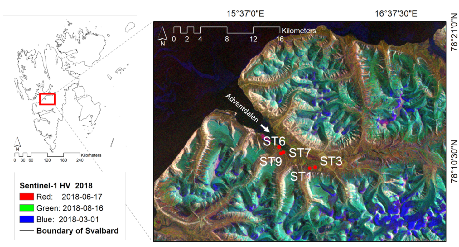
Figure 1. Adventdalen valley and the study area as shown by the Sentinel-1 HV channel in a RGB composition: 17 June 2018 Red band; 16 August 2018 Green band; 1 March 2018 Blue band. The location of the study area on Svalbard (the white arrow points to the Adventdalen valley) and the five selected ground stations are shown.
Remotesensing 14 01866 g001
Figure 2. Images recorded on 27 July 2018 from stations (a) ST1, (b) ST3, (c) ST6, (d) ST7, and (e) ST9.
Remotesensing 14 01866 g002
Figure 3. Flow chart of the proposed approach to detect the main features of snow season and phenology.
Remotesensing 14 01866 g003
Figure 4. Distribution of Ratio values (dB) in snow covered and snow-free condition.
Remotesensing 14 01866 g004
Figure 5. Sentinel-2 RGB images of 2018-07-30 (a) with overlapped in green the snow mask obtained using an NDSI threshold (b), and in yellow the wet snow mask obtained with 2.8 threshold on sigm a 0 (c).
Remotesensing 14 01866 g005
Figure 6. Surface (km 2 ) covered by wet-snow during the melting season 2017 and 2018. The range of days expressed in DOY (from approximately DOY 130, which corresponds to early May, to DOY 250, which corresponds to early September) represents the window in which Sentinel-2 images are usable due to polar night.
Remotesensing 14 01866 g006
Figure 7. Surface [km 2 ] free of snow during the season 2017 and 2018.
Remotesensing 14 01866 g007
Figure 8. Snow cover classification of Sentinel-1 and Sentinel-2, based on backscatter and NDSI thresholds. The two maps at the top represent the month of May (DOY 143 2017 (a) and DOY 144 2018 (b)). In the lower part represents the month of August (DOY 215 2017 (c) and DOY 216 2018 (d)).
Remotesensing 14 01866 g008
Figure 9. Time series of S-1 HV channel and ground sensors for the area ST3 2017: in the graphs, in red is shown the HV backscatter, in green the NDVI, in blue the Soil Water Content (SWC) and in purple the soil temperature at 10 cm depth. A moving average filter was applied to the time series.
Remotesensing 14 01866 g009
Table 1. Description of ground stations location (UTM zone 33 north, datum WGS84), equipment and vegetation in Adventdalen during season 2017 and 2018.
StationUTM XUTM YVegetation and Site DescriptionSensors
ST15236208677555Moist moss tundra with Alopecurus ovatus,
Bistorta vivipara and Salix polaris.
Depressions with Equisetum arvense,
patches of Saxifraga hirculus,
and scattered Dupontia fisheri
and Eriophorum scheuchzeri.
Vegetation cover: 100%
NDVI sensor, soil temperature/moisture,
Infrared radiometer, PhenoCams
ST35244618677707Mosaic of the shrub Dryas octopetala,
and graminoids, e.g., Luzula confusa,
Poa pratensis alpigena and Alopecurus ovatus.
Lots of Salix polaris and Bistorta vivipara on
moist to wet moss tundra dominated by silty sand.
Small landscape feature dominated by soil frost
polygon with little vegetation in the center. Vegetation cover: 90–100%
NDVI sensor, soil temperature/moisture,
Infrared radiometer, PhenoCams
ST65190088680756Grass dominated sandy sediment plain.
Festuca rubra, Poa pratensis ssp alpigena,
and Alopecurus ovatus.Thin organic layer,
with lots of Salix polaris
in between the grasses.
Vegetation cover: 80–100%
NDVI sensor, soil temperature/moisture,
PhenoCams
ST75196558679964Wetland vegetation on flat silty and sandy substrate,
dominated by large polygon soil patterns.
Puccinellia phryganodes, Dupontia fisheri
and Eriophorum scheuchzeri in the interior
part of polygons, while Ranunculus pygmeaus
and bryophytes such as Scorpidium cossonii
and Scorpidium revolvens dominate the wettest
part in polygon cracks. Vegetation cover: 100%
NDVI sensor, soil temperature/moisture,
PhenoCams
ST95192808679794Heath dominated by Luzula confusa.
Other species present are Salix polaris,
Poa pratensis alpigena, Cerastium arcticum
and bryophytes such as Sanionia uncinata
and Tomentypnum nitens.
Some cryoturbation and silty soil.
Vegetation cover: 70–100%
NDVI sensor, soil temperature/moisture,
PhenoCams
Table 2. Sentinel-1 master images and meteorological data years 2017–2018.
Image DateSnow Depth (cm)Air Temperature Mean ( C)Air Temperature Max ( C)Air Temperature Min ( C)Precipitation (mm)
6 March 20179−11.8−7.2−13.3-
12 March 20179−16.9−14.9−21.50.4
24 March 201712−11.2−8.9−12.51.6
10 July 2017-7.48.75.7-
22 July 2017-8.310.95.9-
3 August 2017-8.110.67.4-
17 February 201821−16.3−10.4−22.6-
7 March 201813−16−13.9−16.7-
13 March 201814−18.3−14.8−20.4-
Table 3. First snow-free Day Of Year (DOY) detected by ground station and S-2 snow masks. The 2018 ground stations acquired data staring from May 23, already a snow free period. For this reason only the information of the climatic station (SN99870) was available.
StationGround SensorsSnow Mask
SN99870-2017150 (30 May)142 (22 May)
ST1-2017151 (31 May)154 (3 June)
ST3-2017150 (30 May)146 (26 May)
ST6-2017141 (21 May)144 (24 May)
ST7-2017152 (1 June)147 (27 May)
ST9-2017154 (3 June)166 (15 June)
SN99870-2018128 (8 May)124 (4 May)
Table 4. Pearson correlation coefficient (R) and p-value for the five stations.
Time SeriesStationPearson 2017p-Value 2017Pearson 2018p-Value 2018
S1 HV ∼ NDVIST10.360.0000.520.000
ST30.090.3790.230.014
ST60.640.0000.690.000
ST70.450.0000.560.000
ST90.530.0000.140.147
S1 HV ∼ SWCST10.170.0940.610.000
ST30.810.0000.710.000
ST60.420.0000.530.000
ST7 0.34 0.000 0.34 0.000
ST90.440.0000.650.000
S1 HV ∼ TempST10.380.0000.190.047
ST30.300.0020.190.043
ST60.790.0000.320.000
ST70.770.0000.500.000
ST90.680.000 0.12 0.195
Table 5. Dominance analyses of the linear models between HV ∼ NDVI and HV ∼ SWC.
Station 2017 NDVI %  2017 SWC%   2018 NDVI%  2018 SWC%
ST187134258
ST3199892
ST671296436
ST764367426
ST95941298
Publisher’s Note: MDPI stays neutral with regard to jurisdictional claims in published maps and institutional affiliations.

