On the Joint Exploitation of Satellite DInSAR Measurements and DBSCAN-Based Techniques for Preliminary Identification and Ranking of Critical Constructions in a Built Environment

Abstract

The need for widespread structural safety checks represents a stimulus for the research of advanced techniques for structural monitoring at the scale of single constructions or wide areas. In this work, a strategy to preliminarily identify and rank possible critical constructions in a built environment is presented, based on the joint exploitation of satellite radar remote sensing measurements and artificial intelligence (AI) techniques. The satellite measurements are represented by the displacement time series obtained through the Differential Synthetic Aperture Radar Interferometry (DInSAR) technique known as full resolution Small BAseline Subset (SBAS) approach, while the exploited AI technique is represented by the Density-Based Spatial Clustering of Applications with Noise (DBSCAN) methodology. The DBSCAN technique is applied to the SBAS-DInSAR products relevant to the achieved Persistent Scatterers (PSs), to identify clusters of pixels corresponding to buildings within the investigated area. The analysis of the deformation evolution of each building cluster is performed in terms of velocity rates and statistics on the DInSAR measurements. Synthetic deformation maps of the areas are then retrieved to identify critical buildings. The proposed methodology is applied to three areas within the city of Rome (Italy), imaged by the COSMO-SkyMed SAR satellite constellation from ascending and descending orbits (in the time interval 2011–2019). Starting from the DInSAR measurements, the DBSCAN algorithm provides the automatic clustering of buildings within the three selected areas. Exploiting the derived deformation maps of each study area, a preliminary identification and ranking of critical buildings is achieved, thus confirming the validity of the proposed approach.

1. Introduction

The need for widespread structural safety checks, dictated by the high vulnerability of the built heritage in different countries of the world, constitutes a stimulus for the research of advanced techniques for structural monitoring in a built environment. In the last decades, the satellite measurements obtained by applying the Differential Synthetic Aperture Radar (SAR) Interferometry (DInSAR) technique have given a great impulse to detect superficial deformations, also in the field of the structural engineering. The processing of satellite SAR data permits to obtain ground deformation measurements and thus to detect superficial deformations caused by slow-moving displacement phenomena (on the order of some cm/year), of both natural (e.g., subsidence [1,2], landslides [3,4,5,6,7,8], ground consolidation [9]) and anthropic (e.g., excavations [10], raw materials extraction [11]) origin. These data can be also used to evaluate the vulnerability of systems of constructions under different hypotheses [12,13]. We remark that the DInSAR technique has been widely used for the large-scale analysis of deformation phenomena [14,15,16,17,18]. More recently, the possibility of its application in the field of structural monitoring and assessment has been exploited [1,2,3,5,6,7,8,9,19,20], thanks to the increasing number of Earth Observation (EO) satellites in the orbit and to the high frequency of their data sampling. Note that, compared to the traditional monitoring techniques, satellite DInSAR allows covering much larger areas over a longer time span and without the need to install ground instrumentation, resulting in limited costs. Moreover, the possibility to carry out retrospective analyses to investigate the deformative evolution of an area of interest through the generation of time series, by accessing to satellite data acquired down to 1992, enriches the potentialities of this methodology.

The management and elaboration of satellite data require the use of advanced and effective processing tools, because of their huge volumes and dynamism, continuously increasing in time. In this scenario, machine learning techniques can be implemented for the extraction of information related to the temporal evolution of the measurement points, for their clustering and the generation of the corresponding deformation maps. It is worth noting that the worldwide literature regarding the combined use of satellite SAR data and artificial intelligence (AI) techniques, aimed at structural monitoring, is very scarce. Despite this, the intuition of applying machine learning techniques is supported by successful applications in the research field of the automatic extraction of building footprints in urban areas from point clouds. Indeed, Zhang et al. [21] presented an algorithm for the extraction of building footprints from LIDAR measurements, focusing more on two-dimensional (2-D) footprint extraction than 3-D building models. Then, the majority of the existing approaches derives from largescale airborne laser scanning point clouds. Aljumaily et al. [22] extracted the urban objects from a digital surface model created from aerial laser scanning data, with a fully automatic approach that takes raw 3D points and converts them into sets of clusters through Density-based Spatial Clustering of Applications with Noise (DBSCAN), where each cluster represents an object, such as a building or a portion of a ground surface. Zhang and Zhang [23] proposed a deep learning-based classification algorithm that integrates different neural networks to classify the point clouds into categories of interest, including trees, buildings, and ground. More recent works propose automatic feature extraction methods using remote-sensing-derived products. Guo et al. [24] proposed a point cloud extraction method based on the DBSCAN algorithm, using Tomographic Synthetic Aperture Radar (TomoSAR) point clouds. Finally, Rahimzad et al. [25] proposed an application to multi-sensor remote-sensing images with a new unsupervised feature learning method for efficient urban image clustering.

Within the described research scenario, this work presents a methodology for the extraction of cloud points (representing the buildings of the area) from datasets of satellite DInSAR deformation time series relative to a chosen area, by applying the AI techniques referred to as clustering methods, allowing to identify groups of similar instances in a multivariate dataset (the so-called “clusters”). Then, the retrieved deformations are processed and exploited for the identification of critical constructions of an investigated area that could need further and more in-depth investigations.

In particular, the implemented methodology is applied to three different areas in the city of Rome (Italy), imaged by the X-band COSMO-SkyMed SAR satellite constellation. The generated DInSAR products (deformation time series and mean displacement velocity maps relevant to the coherent points, referred to as Persistent Scatterers—PS) are used as input data, and the DBSCAN clustering method is applied in order to identify the buildings existing in the areas. In this context, an attempt to properly set the DBSCAN hyper-parameters and to integrate the clustering method by means of additional steps that take into account the real distribution of the measuring points, is presented. Then, for each cluster, the deformation condition in the monitored period is analyzed and plotted in maps. This is very useful for the identification of the relative stability among the buildings in the area.

The results of the experiments show that the clusters (buildings) are successfully detected through the proposed approach, and the achieved deformation maps of the areas are effective for the identification of the critical buildings needing further and in-depth investigations. Thereafter, a more advanced structural monitoring for the buildings in critical situations is suggested. For example, in situ inspections and traditional monitoring could be carried out, and on-site information could be integrated with DInSAR measurements.

The paper is organized as follows. Section 2 describes the materials and the methods of the proposed methodology. In particular, Section 2.1 and Section 2.2 highlight, respectively, the key aspects of the DInSAR and DBSCAN techniques and their specific features for civil engineering applications; moreover, Section 2.3 is devoted to the description of the proposed methodology for the preliminary identification and ranking of the critical constructions in urban areas, based on the joint exploitation of the satellite DInSAR measurements and DBSCAN-based techniques. In Section 3, the application of the proposed methodology to three different study areas relevant to the city of Rome (Italy), imaged by the COSMO-SkyMed SAR constellation from ascending and descending orbits during the 2011–2019 time interval, is presented, deeply discussed, and validated. Section 4 contains the discussions on potential and limits of the proposed methodology, whereas Section 5 reports the conclusive remarks.

2. Materials and Methods

In this section, materials and methods used in this work are presented. The materials are analyzed in Section 2.1 and Section 2.2. In particular, Section 2.1 presents the key aspects of the exploited advanced DInSAR technique for the generation of deformation time series, with a focus on the satellite data features most meaningful for civil engineering applications. In Section 2.2, instead, an overview of the DBSCAN clustering algorithm is presented. Finally, Section 2.3 explains all the steps of the proposed methodology for the buildings clustering through the DBSCAN-based algorithm and the preliminary structural monitoring of predefined areas, to identify and make a ranking of the critical constructions.

2.1. DInSAR Technique

DInSAR is one of the most used remote sensing techniques. It is based on the processing of high-resolution radar image pairs acquired through the Synthetic Aperture Radar (SAR) system [26] over an area of interest and allows to derive the magnitude of the displacement component projected along the sensor line of sight (LOS). The effects of additional phase components (e.g., related to changes in the electromagnetic characteristics of the targets on the ground in the time interval of observation, to geometric distortions, to the orbital information inaccuracy, or to changes in atmospheric conditions between the acquisitions) are minimized by taking advantage from the use of the Multi-Temporal DInSAR techniques, such as the Small BAseline Subset (SBAS) approach [27] that, starting from the appropriate processing of a large number of interferometric SAR data pairs, allows to generate mean deformation velocity maps extended over several hundred thousand of km² and, for each coherent point [28], provides the temporal evolution of the displacements occurred in the period of interest by means of the deformation time series. The SBAS technique is able to perform deformation analyses at different spatial resolution scales, producing displacement time series and velocity maps at both regional and local resolution scales [28,29,30]. In particular, when operating at local scale, e.g., for the monitoring of buildings and infrastructures, full resolution differential interferograms generated from the single-look SAR data (characterized by a spatial resolution of the SAR sensor ranging from 3 to 10 m), are employed.

Generally, the SBAS-DInSAR products have an accuracy of 1–2 mm/year on the measurement of the mean displacement velocity, and of 5–10 mm on the single measurement of displacement [31,32,33,34]. The full resolution SBAS-DInSAR technique provides a large set of measuring points for the investigated area, called Persistent Scatterers (PSs), each of which representative of a portion of surface. The interferometric measurements are always calculated with respect to a defined reference point, whose displacement value directly impacts all the points of the dataset.

For each PS, a set of information is provided, made of geographical coordinates (latitude and longitude), height with respect to a global reference system, LOS directional cosines, LOS mean deformation velocity in the overall acquisition period, and LOS displacement measures in each acquisition time. Moreover, the quality of the results from an interferometric point of view is estimated through the temporal coherence value ([28,35]).

The accuracy in the planimetric geolocation of the PSs is related to the estimation of residual topography compared to the Digital Elevation Model (DEM) used in the interferometric processing.

For the same area, ascending (ASC) and descending (DES) measurements may be generally available, with the satellite moving along the acquisition orbits from South to North, or from North to South, respectively. The two datasets can be combined to obtain the deformation components along global directions, commonly East-West (EW) and vertical (z) [36]. It is worth specifying that the deformation along the North-South (NS) direction can be overlooked, accepting a limited error, since the sensor is not quite sensitive to the measurement of the components along this direction. This is because of the lateral view and of the near polar orbit trajectories of the satellite system. Indicating the mean yearly deformation velocity with V, the following system can be written:

$$\{\begin{array}{c}{V}_{ASC}\cong V_{EW}·n_{EW,ASC}+V_V·n_{z,ASC} \\ V_{DES}\cong V_{EW}·n_{EW,DES}+V_V·n_{z,DES}\end{array},$$

(1)

where $n_{EW,ASC/DES}$ and $n_{z,ASC/DES}$ are the directional cosines of the sensor LOS. The system (1) is a simplification of the complete system that is composed by a number of unknown elements (V_EW, V_NS, and V_z) greater than the number of Equation (2), taking into account also the NS component. Equation (1) should be applied to pairs of spatially coincident ASC and DES points. The spatial coincidence of ASC and DES PSs is almost impossible, but the composition can be also performed using pairs of points that can be considered representative of the same reflective target, contemplating a very limited positioning error. For practical purposes, the interferometric products are usually returned as structured ASCII files that can be easily managed in a code language such as python.

The satellite data used in this work, acquired through the standard Stripmap mode, derive from the Italian COSMO-SkyMed (CSK) X-band satellite constellation. For the CSK Stripmap mode data, on average, the portion of surface has a full spatial resolution of about 3 m × 3 m. For a CSK dataset composed by over 100 images, processed at full spatial resolution and with a mean look angle of about 33°, the precision values corresponding to one standard deviation (1σ) are the following: about 1–2 m, 2–3 m, and 1–2 m in the N-S, in the E-W and in the vertical directions, respectively.

2.2. DBSCAN Technique

Clustering methods are AI techniques aimed to identify groups of similar instances in a multivariate dataset: the so-called clusters. Among the different approaches existing in the literature, the density-based clustering methods perform the cluster identification by exploiting the idea that a cluster is a contiguous region of high point density in a data space, whereas low density regions represent noise.

One of the most powerful density-based clustering methods is surely the abovementioned Density-based Spatial Clustering of Applications with Noise (DBSCAN) introduced by Ester et al. [37] in 1996. In short, the DBSCAN algorithm works by considering three types of points: core points, density-reachable points and outliers. In detail, a point in some space to be clustered can be identified as core point if it is characterized by at least a minimum number of points (minPoints) within a selected distance (eps). As for density-reachable points, they are points reachable from a core point through a path, such as p₁, p₂, …, p_n, where p₁ is a core point and p_n is the density-reachable point. A point that is not reachable from any other point is classified as outlier, i.e., it represents noise.

The workflow of the DBSCAN is presented below. DBSCAN starts with randomly selecting a point B. Then, it collects all the points within a space with center B and radius eps. This space is referred as to the neighborhood of the point B. If the neighborhood of the point B does not contain a number of points equal to minPoints, the point B is marked as an outlier. Otherwise, the algorithm creates a first cluster containing B and all points density-reachable from it. In turn, the new points are marked as core points if their eps-neighborhood contains at least a minPoints number of points, and the points density-reachable from them are added to the cluster. In brief, the cluster is built, incrementally, by adding all the points density-reachable from a core point already present in the cluster. The cluster is complete when there are no other points that can be added. This occurs when the new added points are not core points. Once a cluster is completed, the DBSCAN algorithm selects a new random point out of the already completed clusters and repeats the process. It is worth noting that a point recognized as outlier can be found in the neighborhood of a different point and can be introduced in the cluster of this point. Therefore, only at the end of the algorithm process, it is possible to definitely mark a point as outlier. By analyzing how DBSCAN works, there is a clear need to opportunely set two hyper-parameters: the radius of the neighborhood, eps, and the minimum number of points required inside of a cluster, minPoints. Figure 1 reports an example to clarify the functioning of the DBSCAN algorithm [38].

DBSCAN algorithm is one of the most cited density-based clustering methods in the literature. It has been successfully used in several domains, such as urban planning, traffic congestion management and anomaly detection [39]. In the context of spatially extended data, DBSCAN has been already used for dealing with LiDAR data [40,41] and Terrestrial Laser Scanning Data [42]. The main advantage of this clustering algorithm is the ability to discover clusters of arbitrary shapes in spaces of any dimension and effectively identify noise points. Starting from this analysis, DBSCAN seems a suitable approach for achieving one of the goals of this paper, that is, the identification of buildings by exploiting data acquired by means of the SBAS-DInSAR technique, without knowing a priori the number of buildings in the area, their shape, and the dimension of the initial dataset.

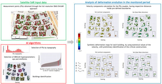
2.3. Proposed Methodology

This section presents the proposed methodology for a preliminary identification and ranking of the critical constructions in urban areas, based on the joint exploitation of satellite DInSAR measurements and DBSCAN-based techniques.

The flowchart of the methodology, shown in Figure 2, is composed of three elements:

➢

The first one (green box) regards the acquisition and the processing of the SAR images relevant to the analyzed area, in the period of interest (in this case, CSK images in the period 2011–2019). The images are processed through a multi-temporal DInSAR technique (in this case, the well-known full resolution SBAS-DInSAR algorithm), in order to obtain spatially dense maps of coherent measurement points (referred to as PSs);

➢

The second one (red box) regards the clustering operation performed by using the DBSCAN algorithm. The identified clusters represent the different buildings of the investigated area;

➢

The third one (blue box) regards the analysis of the deformation evolution of each building in the observation period, by analyzing the velocity trends and statistics of the PSs belonging to the cluster-identified buildings. This allows, through the retrieval of synthetic deformation maps of the investigated area (with focus on the buildings), to carry on a preliminary identification and ranking of critical buildings to be further investigated.

Figure 2. Flowchart of the proposed methodology.

Figure 2. Flowchart of the proposed methodology.

The main characteristics of the satellite input data relevant to the first step of the proposed methodology, i.e., the DInSAR products obtained through the exploited full resolution SBAS technique, have been already explained in detail in Section 2.1. The other two main blocks of the procedure sketched in Figure 2 are described in detail hereafter.

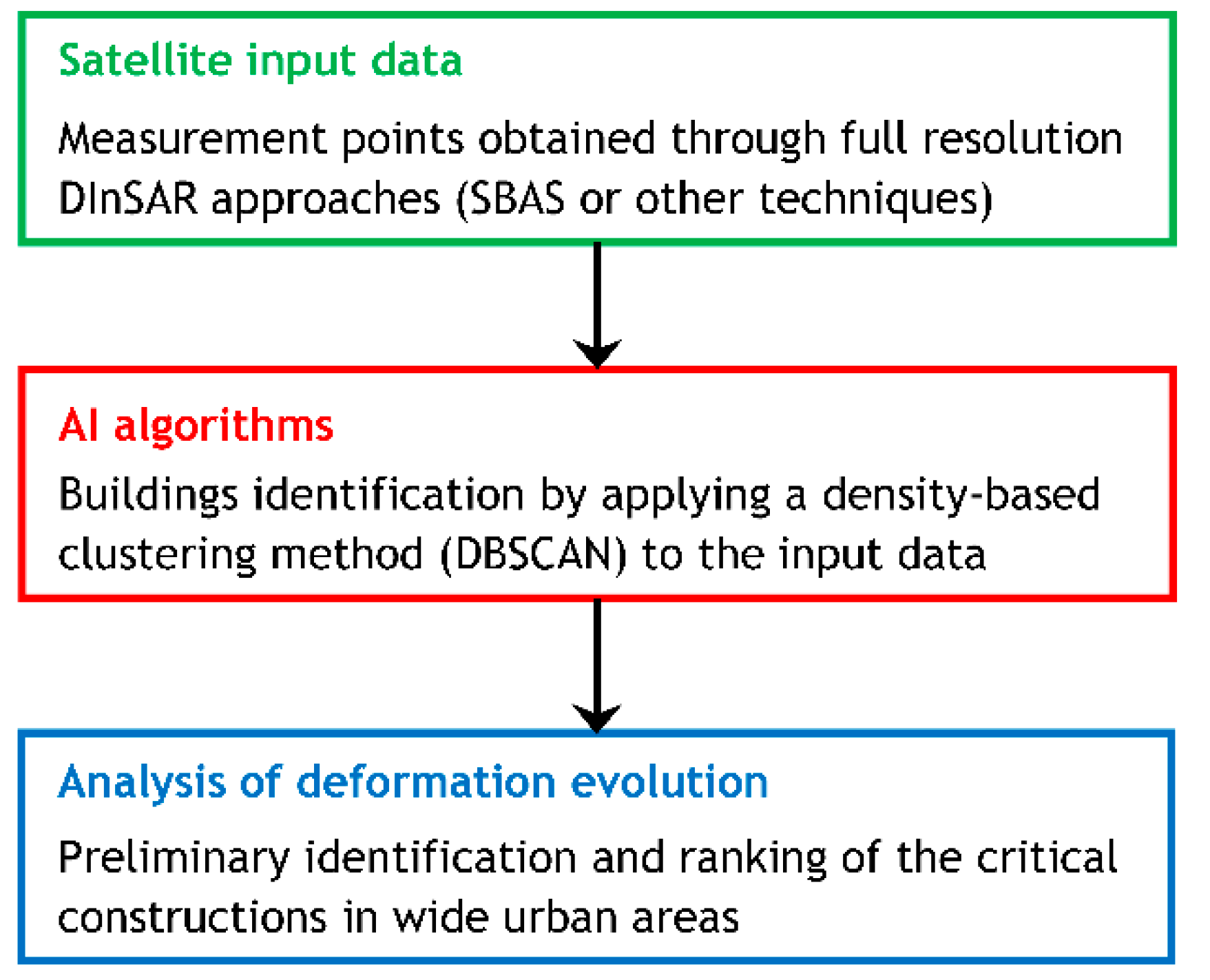
2.3.1. Buildings Identification through DBSCAN Algorithm

This section explains how the existing buildings can be identified starting from the ascending and descending datasets of PSs (merged in order to maximize the PSs density), by means of an AI algorithm based on DBSCAN and improved through additional conditions derived by engineering considerations.

Other than isolated buildings, in urbanized areas, it is very common to find two or more buildings, with a common wall or separated by a seismic joint, only. It is worth noting that the proposed approach does not allow to distinguish single units but, in the abovementioned cases, the structural aggregate is considered as a single “building”.

The flowchart presented in Figure 3 describes the building identification through the DBSCAN algorithm.

With respect to the flowchart shown in Figure 3, the first step of the procedure regards the selection of the PSs by topography (red continue box). It is worth noting that the PSs distribution is usually very heterogeneous in an urban zone: the buildings generally have good reflective properties, so it is very common to detect a density of PSs falling on them. In the areas between buildings, indeed, the PSs are most likely relative to the ground, so, for the purposes of this work, they represent noise and have to be neglected. For this reason, particular attention has to be given to the height of the PSs, δ. The value of δ under which all the PSs are considered to be on the ground surface, is estimated. For the choice of this value, the distribution of the frequency of δ for the dataset of the examined area is observed. In particular, attention is paid on the δ value that shows a first decrease of frequency with respect to the previous one. All the PSs, which have δ values less than the value identified as the upper limit, are supposed to be at the ground level and shall be discarded. The ground level is considered to have a topography given by the δ mean value of all the discarded PSs. An additional vertical error of ± 2 m is considered, corresponding to about one standard deviation, as specified in Section 2.1. The latter, summed to δ associated to the ground PSs, led to the definition of the value under which all the PSs are neglected for the clustering. Moreover, since the one-floor point positioning can show an overlap with the ground points (because of the mentioned possible errors of positioning), an additional δ can be considered, equal to the height of the one-floor buildings (e.g., 3.00–3.50 m, based on the engineering judgment of the user). This limit of the approach will be discussed in Section 4. The clusters constituted by the one-floor buildings could be identified by implementing a second cluster after the first above-described one, by opportunely setting the cut on δ and the other parameters described herein.

Once the first noise cut is done through the topographic considerations, the clustering algorithm DBSCAN can be implemented (red dashed box of the flowchart in Figure 3). As described in Section 2.2, the DBSCAN needs the setting of the two hyperparameters: eps distance and minPoints. The optimal value for neighborhood radius eps is generally determined through an approach consisting in plotting the mean of the distances between each point and its kth nearest neighbor, sorted in ascending order, where k is generally equal to minPoints [43,44]. Then, the optimal value for eps corresponds to the point of maximum curvature of the obtained graph. In this work, to have a better estimation based on the observation of the domain, eps has been evaluated for different values of k, ranging in the interval [k_inf; k_sup], where the boundaries are related to the PSs density of the examined area, obtained by dividing the number of PSs for the corresponding area occupied by buildings. In particular, k_inf has been obtained by multiplying the number of PSs in a m² for the minimum unity surface. The parameter k_sup, instead, has been obtained by multiplying the number of PSs in a m² for a mean area of the buildings in the area. Then, for each value of k included in the interval [k_inf; k_sup], a curve can be drawn, and the point of maximum curvature can be found. Finally, the mean of the ordinates of the retrieved points gives the optimal value for eps. Anyway, the value of eps shall be greater than the minimum distance between the buildings of the area (known or estimated). With respect to the minPoints, instead, according to Ester et al. [34], the DBSCAN default value is 4 for 2-dimensional data. For data with more than 2 dimensions, according to Sander et al. [45], minPoints is computed as: minPoints = 2*dim, where dim is the dimension of the dataset.

At the end of the clustering operations, a plot of the cluster results with building identification is created (red dotted box of the flowchart in Figure 3). As additional check to remove unexpected noise, the users can choose to reject the clusters with less than a minimum area (for example, the minimum unity surface of the building according to local regulations). Each cluster is framed by a rectangle, to delimit the boundary between one cluster and another.

2.3.2. Preliminary Identification and Ranking of Critical Constructions

In this section, the third part of the methodology is described. The flowchart shown in Figure 4 describes the procedure for the preliminary structural monitoring and ranking of the critical constructions in a built environment.

The first two boxes of the flowchart in Figure 4, bounded by solid blue lines, represent the initial steps of the proposed preliminary structural monitoring procedure. For each building, each cluster is sub-divided into two sub-groups, according to the fundamental features (ASC and DES orbits). The relative distances between all the ASC and DES PSs of each cluster are analyzed. Only the couples of points constituted by one ASC and one DES PS, having planimetric and altimetric distances less than the values of error reported in Section 2.1, at once, are considered for the next steps. For the selected couples, the values of the velocity components V_V and V_E-W are calculated according to Section 2.1 and plotted using a symbology with graduated colors. The values of V_V and V_E-W are associated to a new point, spatially located in a mean position with respect the original PSs forming the pair.

Then, the second step regards the analysis of the deformation evolution in the monitored period by using the velocity components of the selected couples with the goal of providing a preliminary structural monitoring through the ranking of the criticalities (blue dashed box of the flowchart in Figure 4). In this phase, some statistical values of the velocity components are recognized in each cluster: the maximum (V_V,max, V_EW,max), the minimum (V_V,min, V_EW,min), and the mean velocity weighted on the values of the temporal coherence. Moreover, the maximum (V_V,max, V_EW,max) and the minimum (V_V,min, V_EW,min) values allow to understand if the building is interested by differential displacements, and to estimate the differential velocity amount in the considered direction. The resulting component maps are a very useful tool to easily identify the buildings most affected by displacements, and to identify critical situations, if existing. The definition of a critical building such as the actions to be taken when this condition is present will be discussed in Section 4, since they are out of the scope of this paper. Generally, once the most exposed buildings are identified, the third phase can be activated for them (blue dotted box of the flowchart in Figure 4). In this phase, it is important to combine on-site information for the single critical building or for the entire area (traditional measurements and geometrical and structural relief of the buildings) with more building-specific DInSAR measurements.

3. Results

The proposed approach has been applied to three macro-areas, as shown in this section. To implement the proposed approach, python code-language has been used, and the available libraries have been exploited to speed-up the process and reduce the possible errors.

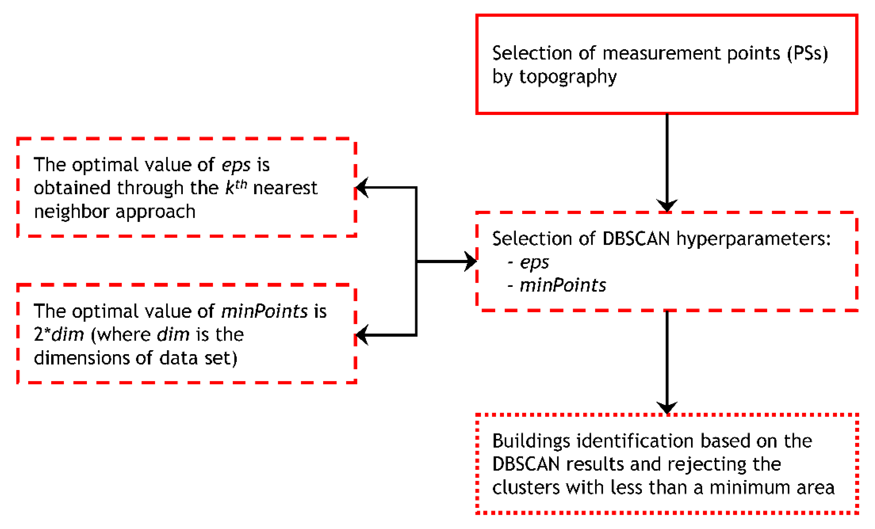
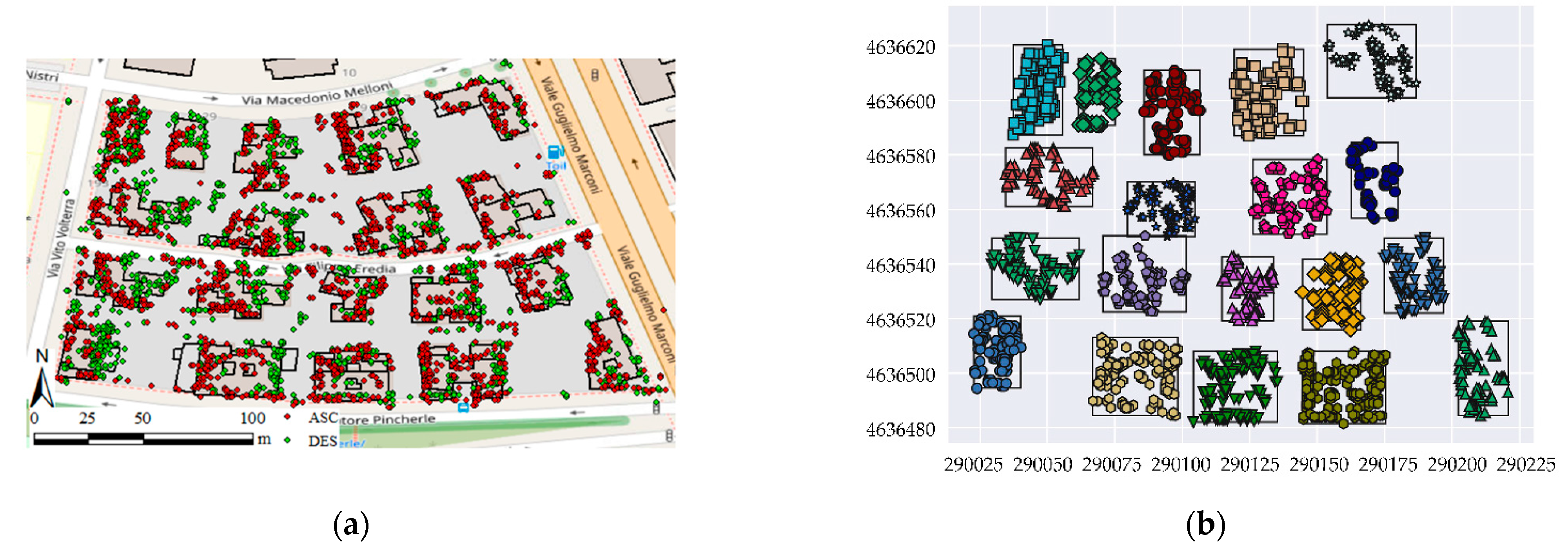
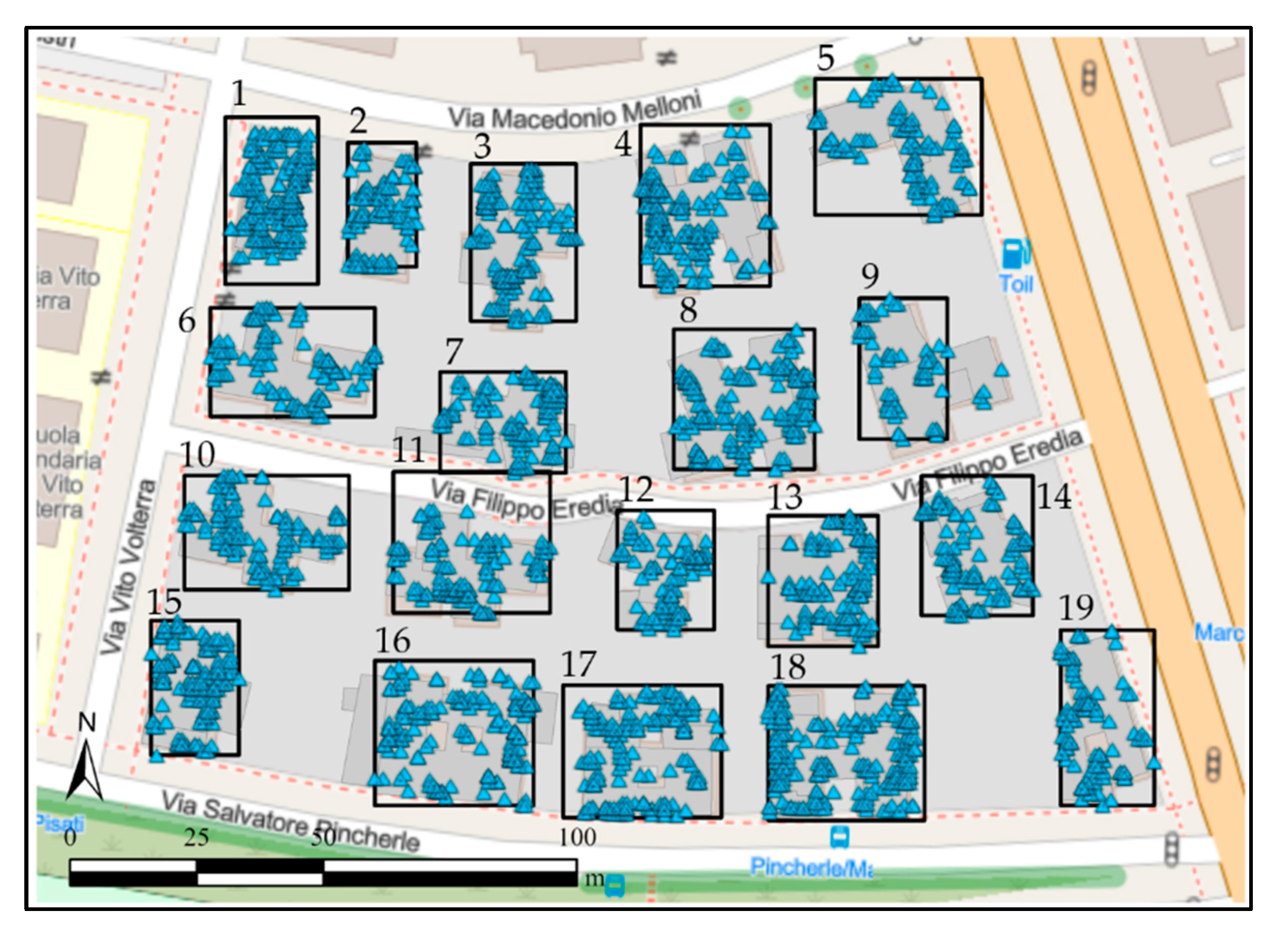
3.1. Case Study Areas

The case study areas are part of the municipality of Rome (Italy) which is entirely interested by an extensive multi-temporal interferometric processing [2,20,36,46,47,48,49]. In particular, with reference to the whole urban area, the full resolution SBAS-DInSAR approach ([28,30]) has been applied to two sets of SAR images collected from 2011 to 2019, from ASC and DES CSK orbits. The three areas differ for many characteristics: width (m²), number of buildings, planimetric shape, and number of floors of the buildings (Figure 5).

3.2. Algorithm Application and Clustering Results

3.2.1. Selection of PSs by Topography

The distributions of the frequency of all the PSs δ for the three areas are shown in Figure 6. In this work, a reasonable value of 30% has been set as limit of frequency variation. For Areas 1 and 3, a decrease of frequency larger than 30% can be observed between 2–4 m and 4–6 m, while for Area 2, it occurs between 4–6 m and 6–8 m. A detail of the topography values considered for each area is reported in

Table 1. Topography ground level δ and δ limit values.

Area Number [-]	Ground Level δ [m]	δ Limit [m]
1	2.59	8.09
2	2.78	8.28
3	2.64	8.14

. With the δ limit, it is indicated the value under which the PSs are neglected for the clustering, obtained by summing the standard deviation (σ = ±2 m) and the supposed height of 1-floor buildings (3.50 m) to the ground level measure δ.

3.2.2. Selection of DBSCAN Hyper-Parameters

For all the areas, the minimum samples value minPoints has been set at 4, since the dataset used in this work has 2 dimensions. As regards eps, the approach mentioned in Section 3.1 has been implemented for the three areas. The results are shown in Figure 7, both in terms of plots of the mean of the distances between each point and its kth nearest neighbor, sorted in ascending order, and reporting the information needed to find the eps: the numbers of ASC and DES PSs, and their sum (tot. PSs), the area, the PSs density (PSs/m²), the boundaries k_inf and k_sup, and, finally, the optimal value for neighborhood radius eps. The latter has been estimated as the mean of the ordinates of the maximum curvature points (represented with red circular markers) referred to each curve, given by a value of k included in the interval [k_inf; k_sup]. According to Section 2.3.1, the ends of this interval are estimated based on a PSs density obtained by dividing the number of PSs for the area occupied by buildings, approximately the 50% of the total area for the case study areas. Then, k_inf has been obtained by multiplying the number of PSs in a m² for the minimum unity surface, set at 28 m² in this case, according to the Italian D.M. 05/07/1975 [50]. The value of k_sup, indeed, has been evaluated taking into account that the greater distribution is generally on the roof, and other PSs can be found on the facades, so herein, a mean area of the buildings is estimated to be 250 m².

The optimal values obtained for eps are very similar for the three areas. These values are very close to the minimum distance between the buildings. Then, in absence of such analysis, for urban areas with similar features, an eps value between 6 and 7 m could be suggested.

3.2.3. Clustering Results

In Figure 8, Figure 9 and Figure 10, the comparisons between the original PSs dataset distribution in the three areas and the clustering results, are proposed. In Figure 8a, Figure 9a and Figure 10a, the buildings’ footprints are clearly marked with a black shape. There are 19 buildings in Area 1, 12 buildings in Area 2 and 20 buildings in Area 3. Moreover, the PSs, distributed all over the areas, marked with red circles for ascending PSs and green circles for descending PSs, are shown. In Figure 8b, Figure 9b and Figure 10b, the results of the clustering are reported, where each cluster has been delimited by a rectangle. The clustering results have highlighted that the procedure is very performant. Each building having more than one floor is identified by a cluster. The only exception is represented by the one-floor manufact of Area 2, that is not included in the clustering results due to the additional δ considered for the height cut, aimed to avoid noise PSs (belonging to the ground), as previously exposed in Section 2.3.1.

3.3. Potential Application for Structural Monitoring

The procedure described in Section 2.3.2 has allowed to identify all the couples of PSs respecting the criteria to be combined. The velocity components V_V and V_EW have been estimated for each couple, by implementing Equation (1) presented in Section 2.1. In Figure 11, Figure 12 and Figure 13, the maps of V_V and V_EW are shown. The symbology has graduated colors ranging from dark red (downwards and west-directed displacements, respectively) to dark blue (upwards and East-directed displacements, respectively). The green points are representative of stable areas, not affected by displacements.

Synthetic maps have been created from the previous ones, showing for each cluster the significative values of the velocity components. In Figure 14a, Figure 15a and Figure 16a, for the Areas 1, 2 and 3, respectively, the following information is graphically represented: V_V,max and V_V,min, with a star marker, placed in their current position; V_V,mean with a circular marker, placed in the middle of the cluster; the values of V_V,mean ± 1σ, with triangular markers, on the two sides of V_V,mean. Analogous maps are represented for the EW components of velocity, in Figure 14b, Figure 15b and Figure 16b.

In Area 1, an ongoing deformation phenomenon can be observed (Figure 14). In particular, the vertical component is prevailing, showing downward movements. The vertical velocity increases from the top left zone to the bottom right zone. Differential displacements can also be observed in the same building. It is even more evident looking at the summary maps. For example, the last building of the third “row” has a V_V,min value in the yellow range ([−0.3–−0.1] cm/y) and a V_V,max one in the orange range ([−0.3–−0.5] cm/y). In the EW direction, the velocity maps show lower velocity values.

Moreover, in Area 2, an even clearer ongoing deformation phenomenon can be observed (Figure 15). The vertical component is the prevailing one, with downward movements, but the EW component is not negligible in some buildings. The buildings most affected by the vertical deformation phenomenon are those of the southern zone, that reach values of V_V also lower than −0.7 cm/y. Significant displacements can also be observed on some buildings. For example, in the second building on the right, starting from the bottom, the vertical component increases from north to south, while, on the contrary, the EW component decreases from north to south. It is even more evident looking at the summary maps. The examined building, in fact, presents a V_V,min value within the green range ([−0.1–+0.1] cm/y) on the North-East side, and a V_V,max one in the dark red range ([<−0.7] cm/y) on the south side. In the EW direction, it presents a V_{EW,min value} in the orange range ([−0.5–+0.3] cm/y) on the North-East side, and a V_EW,max one in the green range ([−0.1–+0.1] cm/y) on the south-west side.

Finally, Area 3 presents the worst vertical ongoing deformation behavior among the three areas, while the EW component is quite negligible (Figure 16). Among each building, the velocity components are quite homogeneous, so they are not supposed to suffer from differential deformations.

The prevailing vertical velocity trend detected in the three areas is imputable, probably, due to subsidence or consolidation phenomena [47].

3.4. Validation of the Results

The validation of the results obtained through the proposed methodology has been performed with respect to the clustering that represents the novelty of the work. In detail, the performed validation consists of comparing the clustering results, obtained as described in Section 3.2.3 thanks to DBSCAN algorithm, to the point cloud identified, for the same buildings through a detailed analysis of the PSs. Unfortunately, we do not have the ground truth for the considered areas, i.e., the real match between the points and the clusters, and, in general, it is difficult to find datasets with this information. For this reason, in order to carry out our validation, a ground truth has been built by applying a controlled procedure, performed without the aid of AI algorithms. In detail, the performed procedure is characterized by the following steps: (i) the schematic volumes of the building, obtained from the open-source Regional Technical Numerical Map (CTR) of Lazio Region [51], are reconstructed; (ii) all the PSs intersecting the volumes themselves are selected, considering a buffer of 2.5 m around; (iii) as proposed in Section 3.2.1, the PSs having a δ under the δ limit used in Area 1 (see Table 1) are neglected. The procedure is schematically represented in Figure 17, with reference to the building 14 of Area 1 (see Figure 18). The grey volume shows the step (i) of the procedure; then, all the PSs in a buffer of 2.5 m from the edges of the building are considered, according to step (ii); finally, the PSs under a red line at δ height used in Area 1 (see Table 1) are neglected (step (iii)).

Due to the effort related to this procedure, it has been repeated only for the buildings in Area 1. A spatial check has been done, as shown in Figure 18 where the floor plan view of the buildings and the selected PSs are represented. Moreover, the rectangles delimiting the clusters obtained through DBSCAN are also reproposed to highlight, on one side, that there is a general good agreement between the buildings’ plans geometries (from CTR) and the rectangles delimiting the previous clusters, and, on the other side, that almost in every case, the PSs by the validation procedure are included in them. Only in one case, this is not verified: for building no. 9; in fact, 4 PSs are external to the corresponding rectangle. This means that the proposed algorithm had excluded them from the cluster, while the built ground truth includes them. Moreover, the building footprints under the clusters allow observing that some PSs belonging to building no. 7 were included in the cluster of building 11 since the 11th rectangle extends to the south side of building no. 7.

The comparison of the results has been done not only in spatial terms, but also in terms of number of PSs included in each cluster. The number of ASC and DES PSs, and the total number of PSs composing the 19 clusters of Area 1, are reported in

Table 2. Clustering results from the proposed methodology.

CLUSTER	1	2	3	4	5	6	7	8	9	10	11	12	13	14	15	16	17	18	19
ASC	75	41	93	124	69	63	43	100	38	65	80	55	63	81	51	70	88	129	63
DES	138	49	70	61	39	63	83	70	18	42	46	46	67	36	95	90	62	92	36
Tot.	213	90	163	185	108	126	126	170	56	107	126	101	130	117	146	160	150	221	99

(results from the proposed methodology) and

Table 3. Clustering results from the validation procedure.

CLUSTER	1	2	3	4	5	6	7	8	9	10	11	12	13	14	15	16	17	18	19
ASC	69	47	88	119	66	61	43	97	42	67	81	47	60	81	50	70	89	125	65
DES	133	48	72	62	39	63	83	74	19	41	47	41	66	35	95	90	63	99	34
Tot.	202	95	160	181	105	124	126	171	61	108	128	88	126	116	145	160	152	224	99

(results for the ground truth). There is a good agreement between the clusters’ composition. Indeed, for 17 clusters out of 19, the difference is contained in the 5%, for cluster no. 9 is 8% and for cluster no. 12 is 15%.

4. Discussion

The DInSAR displacement time series are clearly relevant to a defined time period, which is generally a small portion of the entire lifetime of a construction. At the end of the observation interval, the cumulative displacements can be estimated, and ground settlement profiles referred to the sides of the building under investigation can be created. Classical literature indications could be used to qualitatively evaluate the expected damage caused by such detected displacements. Nevertheless, it is worth highlighting that the latter are related only to the abovementioned satellite data observation period. Then, a real correlation between the expected and the observed damages could be truthful only for structures for which the satellite radar imaging has started at time “zero” of the building construction.

For the purposes of this work, the main importance is given to the displacements’ trend, i.e., the mean velocity in the investigated time interval. The study of the deformation velocity trends can be pursued at wide area or local scale. The trend analysis can support the interpretation of the deformation evolution, giving qualitative information about the movement patterns, aimed at the identification of critical areas or buildings in critical situations, in terms of stability, as illustrated in Section 3.3.

The critical areas could be identified in a widely built environment by automating the steps of the proposed methodology. This could concern two aspects: from one side, a qualitative idea of the extension and entity of possible ongoing phenomena in the area could be retrieved; on the other side, the structures exposed to the phenomena themselves could be spatially bounded and posed under attention. The definition of the conditions that make a building defined as critical can be related to several considerations correlated to many factors of an investigated zone (e.g., geology of the area, ongoing deformation phenomena in the entire area, widespread structural typologies, average construction age of the buildings, etc.). However, exploiting the complete pattern of the deformation velocity trends of all the buildings in the monitored area, differential “attention” thresholds could be imposed regarding: (i) a building showing velocity values greater than those of the buildings around; (ii) a change in the velocity trends of many parts of a building over the observation period; (iii) building sides affected by differential displacements.

Then, once the most exposed buildings are identified, further and more in-depth investigations should be performed. In particular, the satellite DInSAR measurements could be used to perform a structural monitoring at the detail scale, distinguishing the mean velocity values of points at different heights, and obtaining the ground displacement profiles under the building sides or at different heights (e.g., at roof height). Classical literature indications could be used to qualitatively define the expected damage which such detected displacements may cause/have caused [2]. Moreover, these displacement profiles can be applied at the ground level of the selected construction in a numerical model. Then, a structural analysis can be conducted to predict the resulting behavior and to evaluate the damage level in the single members at a local level and in the overall building at a global level, according to the selected code requirements. Finally, in this phase, it is suggested to combine on-site information (traditional measurements, such as GPS, topographic levelling tools, crack meter instrumentation, strain gauges, multi-sensor nodes, and geometrical and structural relief of the buildings) with DInSAR measurements.

Some considerations can be done on the different approaches that could be used to elaborate the information derived from the PSs. In fact, once identified and well positioned the PSs on the building volume, different techniques can be used to investigate the possible displacements of the structure, based on the combination of the ASC and DES datasets (discussed, e.g., in Di Carlo et al. [2] and Talledo et al. [36]), under the assumptions explained in Section 2.1. For example, spatial interpolation techniques can be used for mapping the mean velocity components, under specific hypotheses, to create preliminary deformation maps (as alternative to the procedure performed in this work, based on the selection of PSs couples, only if the PSs have a good spatial density).

One of the limits of the proposed methodology is its inability to sharply distinguish single buildings units, when they are built-in, as hinted in Section 2.3.1. Specifically, from a structural point of view, if two buildings have a common wall, or common structural foundations, they constitute a single structure. In this case, no approximation subsists in the methodology. When two buildings are separated by a seismic joint, instead, they have completely different structural behaviors and do not interact with each other. In this case, it is not possible to distinguish buildings so close through the input satellite data, and an approximation is done. So, if the output clusters are very large, it is suggested to focus on them to understand if it is a single building, or an aggregate, or joined buildings, to make appropriate considerations for the specific case.

Another limit of the proposed methodology is the difficulty in identifying the clusters referred to one-floor buildings, since they are classified as noise in order to avoid the creation of false clusters, as explained in Section 2.3.1. This assumption is necessary since it strengthens the correct identification of the two-to-n floors buildings, by eliminating any interaction with the ground points. Nevertheless, it eliminates the possibility to identify one-floor buildings, and some very few points of the n-floors buildings’ facades. This limit could be exceeded by integrating the proposed clustering algorithm with an additional clustering, to execute by opportunely setting the cut on δ and the eps. For example, the clustering could be repeated excluding only the PSs supposed to be on the ground. Then, the new clusters, not overlapping those obtained through the first clustering, should be added to the previous result. Maybe, in some cases, this second clustering could also help in finding a more refined shape of the two-floor buildings, since some points can be excluded in the initial cut, as consequence of the topographic error. More in-depth studies are in progress to pursuit this scope. However, it is worth noting that it is very rare to find one-floor buildings in very urbanized areas (in fact, as it has been shown in this work, only one has been found in three areas). Then, neglecting them in a preliminary phase is not a very strong limitation.

Finally, it is worth specifying that the clustering result is quite sensitive to small hyper-parameters changes, so the latter should be set with attention.

5. Conclusions

The spread of the advanced DInSAR techniques for the generation of spatially dense deformation time series has highly contributed to the development of several applications, among which we underline those relevant to the structural stability assessment of buildings and infrastructures. On the other hand, within this framework, the large data volumes of the generated DInSAR products need to be properly accounted, when dealing with automatic tools for the extraction of relevant information. In this context, a strong support may derive from the exploitation of the AI techniques, which represent powerful instruments for automatically extracting significant information associated to features. In this work, a methodology, jointly exploiting satellite DInSAR measurements and DBSCAN-based techniques, has been proposed for the preliminary identification and ranking of possible critical constructions in a built-up environment. This methodology has been successfully applied to CSK-based DInSAR time series relevant to three sample areas within the city of Rome (Italy). In particular, the DBSCAN clustering algorithm has allowed the automatic extraction of urban buildings from PSs clouds. Then, for each cluster, an elaboration of the data has led to obtain the picture of the deformation condition in the investigated period, for each considered area. Indeed, by studying the velocity trends and statistics of the PSs belonging to the cluster-identified buildings, synthetic deformation maps of the investigated area (with focus on the buildings) are retrieved, which allow to carry out a preliminary identification and ranking of critical buildings to be further investigated.

Some proposals for future developments aimed to improve the presented methodology are highlighted. The hyper-parameters of the DBSCAN will be refined, to detect the one-floor buildings (that in this work have been neglected). Otherwise, further different clustering algorithms, e.g., OPTICS [52], could be integrated in our methodology. Moreover, fitting methods could be implemented to fit the model through the original SAR images, in order to extract information on buildings by overcoming the clustering step and refine their identification. The clustering results could also be improved, to avoid the inclusion of noise clusters that are not representative of a building but are referred to other elements that reflect the signal emitted by the satellite. This could be accomplished by imposing an additional condition: the clusters which occupy an area lower than a minimum value (assuming a minimum dimensions of a building) could be classified as noise.

Finally, the temporal coherence of the PSs can be considered as a driven parameter in two different ways: (a) a pre-selection on the PSs dataset could be done, considering only the PSs characterized by values of temporal coherence greater than a certain threshold (e.g., 0.6–0.7), to increase the reliability of the results; (b) a post-processing on the statistics of the velocity values can be implemented by weighting the single value for their relative temporal coherence.

The presented approach could give a decisive impulse to the automation of the preliminary structural monitoring of a built environment at a large spatial scale, beyond the specific structural typologies. In particular, the resulting maps could provide support in decisional phases, as well as to the organization of preventive measures to reduce the risks for the built environment associated to the measured deformations. Therefore, the possibility to automatize the imposition of trigger alarms for the areas under investigation through the joint exploitation of satellite and AI techniques could represent a very relevant prevention tool.

The code developed to implement the methodology is available under request, by contacting the authors.

References

1. Arangio, S.; Calò, F.; Di Mauro, M.; Bonano, M.; Marsella, M.; Manunta, M. An application of the SBAS-DInSAR technique for the assessment of structural damage in the city of Rome. Struct. Infrastruct. Eng. 2014, 10, 1469–1483. [Google Scholar] [CrossRef]
2. Di Carlo, F.; Miano, A.; Giannetti, I.; Mele, A.; Bonano, M.; Lanari, R.; Meda, A.; Prota, A. On the integration of multi-temporal synthetic aperture radar interferometry products and historical surveys data for buildings structural monitoring. J. Civ. Struct. Health Monit. 2021, 11, 1429–1447. [Google Scholar] [CrossRef]
3. Infante, D.; Confuorto, P.; Di Martire, D.; Ramondini, M.; Calcaterra, D. Use of DInSAR data for multi-level vulnerability assessment of urban settings affected by slow-moving and intermittent landslides. Procedia Eng. 2016, 158, 470–475. [Google Scholar] [CrossRef] [Green Version]
4. Peduto, D.; Pisciotta, G.; Nicodemo, G.; Arena, L.; Ferlisi, S.; Gullà, G.; Borrelli, L.; Fornaro, G.; Reale, D. A procedure for the analysis of building vulnerability to slow-moving landslides. In Proceedings of the 1st IMEKO International Workshop on Metrology for Geotechnics, Benevento, Italy, 17–18 March 2016. [Google Scholar]
5. Del Soldato, M.; Solari, L.; Poggi, F.; Raspini, F.; Tomás, R.; Fanti, R.; Casagli, N. Landslide-Induced Damage Probability Estimation Coupling InSAR and Field Survey Data by Fragility Curves. Remote Sens. 2019, 11, 1486. [Google Scholar] [CrossRef] [Green Version]
6. Infante, D.; Di Martire, D.; Confuorto, P.; Tessitore, S.; Tòmas, R.; Calcaterra, D.; Ramondini, M. Assessment of building behavior in slow-moving landslide-affected areas through DInSAR data and structural analysis. Eng. Struct. 2019, 199, 109638. [Google Scholar] [CrossRef] [Green Version]
7. Miano, A.; Mele, A.; Calcaterra, D.; Di Martire, D.; Infante, D.; Prota, A.; Ramondini, M. The use of satellite data to support the structural health monitoring in areas affected by slow-moving landslides: A potential application to reinforced concrete buildings. Struct. Health Monit. 2021, 20, 3265–3287. [Google Scholar] [CrossRef]
8. Mele, A.; Miano, A.; Di Martire, D.; Infante, D.; Ramondini, M.; Prota, A. Potential of remote sensing data to support the seismic safety assessment of reinforced concrete buildings affected by slow-moving landslides. Arch. Civ. Eng. 2022, 22, 88. [Google Scholar] [CrossRef]
9. Drougkas, A.; Verstrynge, E.; Van Balen, K.; Shimoni, M.; Croonenborghs, T.; Hayen, R.; Declercq, P.Y. Country-scale InSAR monitoring for settlement and uplift damage calculation in architectural heritage structures. Struct. Health Monit. 2020, 1475921720942120. [Google Scholar] [CrossRef]
10. Giannico, C.; Ferretti, A.; Alberti, S.; Jurina, L.; Ricci, M.; Sciotti, A. Application of satellite radar interferometry for structural damage assessment and monitoring LifeCycle and Sustainability of Civil Infrastructure Systems. In Proceedings of the 3rd International Symphosium on Life-Cycle Civil Engineering (IALCCE ’12), Vienna, Austria, 3–6 October 2012. [Google Scholar]
11. Herrera, G.; Tomás, R.; Vicente, F.; Lopez-Sanchez, J.M.; Mallorquí, J.J.; Mulas, J. Mapping ground movements in open pit mining areas using differential SAR interferometry. Int. J. Rock Mech. Min. 2010, 47, 1114–1125. [Google Scholar] [CrossRef]
12. Miano, A.; Mele, A.; Prota, A. Fragility curves for different classes of existing RC buildings under ground differential settlements. Eng. Struct. 2022, 257, 114077. [Google Scholar] [CrossRef]
13. Nappo, N.; Peduto, D.; Polcari, M.; Livio, F.; Ferrario, M.F.; Comerci, V.; Stramondo, S.; Michetti, A.M. Subsidence in Como historic centre (northern Italy): Assessment of building vulnerability combining hydrogeological and stratigraphic features, Cosmo-SkyMed InSAR and damage data. Int. J. Disaster Risk Reduct. 2021, 56, 102115. [Google Scholar] [CrossRef]
14. Gabriel, A.K.; Goldstein, R.M.; Zebker, H.A. Mapping small elevation changes over large areas: Differential radar interferometry. J. Geophys. Res. 1989, 94, 9183–9191. [Google Scholar] [CrossRef]
15. Massonnet, D.; Feigl, K.L. Radar interferometry and its application to changes in the earth’s surface. Rev. Geophys. 1998, 36, 441–500. [Google Scholar] [CrossRef] [Green Version]
16. Rosen, P.A.; Hensley, S.; Joughin, I.R.; Li, F.K.; Madsen, S.N.; Rodríguez, E.; Goldstein, R.M. Synthetic aperture radar interferometry. IEEE Trans. Geosci. Remote Sens. 2000, 88, 333–380. [Google Scholar] [CrossRef]
17. Lanari, R.; De Natale, G.; Berardino, P.; Sansosti, E.; Ricciardi, G.P.; Borgstrom, S.; Capuano, P.; Pingue, F.; Troise, C. Evidence for a peculiar style of ground deformation inferred at Vesuvius volcano. Geophys. Res. Lett. 2002, 29, 6-1–6-4. [Google Scholar] [CrossRef]
18. Del Soldato, M.; Riquelme, A.; Bianchini, S.; Tomàs, R.; Di Martire, D.; De Vita, P.; Moretti, S.; Calcaterra, D. Multisource data integration to investigate one century of evolution for the Agnone landslide (Molise, southern Italy). Landslides 2018, 15, 2113–2128. [Google Scholar] [CrossRef] [Green Version]
19. Bianchini, S.; Pratesi, F.; Nolesini, T.; Casagli, N. Building deformation assessment by means of persistent scatterer interferometry analysis on a landslide-affected area: The Volterra (Italy) case study. Remote Sens. 2015, 7, 4678–4701. [Google Scholar] [CrossRef] [Green Version]
20. Ponzo, F.C.; Iacovino, C.; Ditommaso, R.; Bonano, M.; Lanari, R.; Soldovieri, F.; Cuomo, V.; Bozzano, F.; Ciampi, P.; Rompato, M. Transport Infrastructure SHM Using Integrated SAR Data and On-Site Vibrational Acquisitions: “Ponte Della Musica–Armando Trovajoli” Case Study. Appl. Sci. 2021, 11, 6504. [Google Scholar] [CrossRef]
21. Zhang, K.; Yan, j.; Chen, S.C. Automatic construction of building footprints from airborne LIDAR data. IEEE Trans. Geosci. Remote Sens. 2006, 44, 2523–2533. [Google Scholar] [CrossRef] [Green Version]
22. Aljumaily, H.; Laefer, D.F.; Cuadra, D. Urban point cloud mining based on density clustering and MapReduce. J. Comput. Civ. Eng. 2017, 31, 04017021. [Google Scholar] [CrossRef]
23. Zhang, L.; Zhang, L. Deep learning-based classification and reconstruction of residential scenes from large-scale point clouds. IEEE Trans. Geosci. Remote Sens. 2017, 56, 1887–1897. [Google Scholar] [CrossRef]
24. Guo, Z.; Liu, H.; Pang, L.; Fang, L.; Dou, W. DBSCAN-based point cloud extraction for Tomographic synthetic aperture radar (TomoSAR) three-dimensional (3D) building reconstruction. Int. J. Remote Sens. 2021, 42, 2327–2349. [Google Scholar] [CrossRef]
25. Rahimzad, M.; Homayouni, S.; Alizadeh Naeini, A.; Nadi, S. An Efficient Multi-Sensor Remote Sensing Image Clustering in Urban Areas via Boosted Convolutional Autoencoder (BCAE). Remote Sens. 2021, 13, 2501. [Google Scholar] [CrossRef]
26. Franceschetti, G.; Lanari, R. Synthetic Aperture Radar Processing, 1st ed.; CRC Press LLC: Boca Raton, FL, USA, 1999. [Google Scholar]
27. Berardino, P.; Fornaro, G.; Lanari, R.; Sansosti, E. A new algorithm for surface deformation monitoring based on small baseline differential SAR interferograms. IEEE Trans. Geosci. Remote Sens. 2002, 40, 2375–2383. [Google Scholar] [CrossRef] [Green Version]
28. Lanari, R.; Mora, O.; Manunta, M.; Mallorquí, J.J.; Berardino, P.; Sansosti, E. A small baseline approach for investigating deformations on full resolution differential SAR interferograms. IEEE Trans. Geosci. Remote Sens. 2004, 42, 1377–1386. [Google Scholar] [CrossRef]
29. Manunta, M.; Marsella, M.; Zeni, G.; Sciotti, M.; Atzori, S.; Lanari, R. Two-scale surface deformation analysis using the SBAS-DInSAR technique: A case study of the city of Rome, Italy. Int. J. Remote Sens. 2008, 29, 1665–1684. [Google Scholar] [CrossRef]
30. Bonano, M.; Manunta, M.; Marsella, M.; Lanari, R. Long-term ERS/ENVISAT deformation time-series generation at full spatial resolution via the extended SBAS technique. Int. J. Remote Sens. 2012, 33, 4756–4783. [Google Scholar] [CrossRef]
31. Casu, F.; Manzo, M.; Lanari, R. A quantitative assessment of the SBAS algorithm performance for surface deformation retrieval from DInSAR data. Remote Sens. Environ. 2006, 102, 195–210. [Google Scholar] [CrossRef]
32. Manunta, M.; De Luca, C.; Zinno, I.; Casu, F.; Manzo, M.; Bonano, M.; Fusco, A.; Pepe, A.; Onorato, G.; Berardino, P.; et al. The parallel SBAS approach for Sentinel-1 interferometric wide swath deformation time-series generation: Algorithm description and products quality assessment. IEEE Trans. Geosci. Remote Sens. 2019, 57, 6259–6281. [Google Scholar] [CrossRef]
33. Manzo, M.; Fialko, Y.; Casu, F.; Pepe, A.; Lanari, R. A Quantitative Assessment of DInSAR Measurements of Interseismic Deformation: The Southern San Andreas Fault Case Study. Pure Appl. Geophys. 2012, 169, 1463–1482. [Google Scholar] [CrossRef]
34. Bonano, M.; Manunta, M.; Pepe, A.; Paglia, L.; Lanari, R. From previous C-band to new X-band SAR systems: Assessment of the DInSAR mapping improvement for deformation time-series retrieval in urban areas. IEEE Trans. Geosci. Remote Sens. 2013, 51, 1973–1984. [Google Scholar] [CrossRef]
35. Hooper, A.; Bekaert, D.; Spaans, K.; Arikan, M. Recent advances in SAR interferometry time series analysis for measuring crustal deformation. Tectonophysics 2012, 514, 1–13. [Google Scholar] [CrossRef]
36. Talledo, D.A.; Miano, A.; Bonano, M.; Di Carlo, F.; Lanari, R.; Manunta, M.; Meda, A.; Mele, A.; Prota, A.; Saetta, A.; et al. Satellite radar interferometry: Potential and limitations for structural assessment and monitoring. J. Build. Eng. 2022, 46, 103756. [Google Scholar] [CrossRef]
37. Ester, M.; Kriegel, H.P.; Sander, J.; Xuet, X. A density-based algorithm for discovering clusters in large spatial databases with noise. Kdd 1996, 96, 226–231. [Google Scholar]
38. Schubert, J.; Sander, M.; Ester, H.; Kriegel, P.; Xu, X. DBSCAN revisited, revisited: Why and how you should (still) use DBSCAN. ACM Trans. Database Syst. 2017, 42, 1–21. [Google Scholar] [CrossRef]
39. Huang, F.; Zhu, Q.; Zhou, J.; Tao, J.; Zhou, X.; Jin, D.; Tan, X.; Wang, L. Research on the Parallelization of the DBSCAN Clustering Algorithm for Spatial Data Mining Based on the Spark Platform. Remote Sens. 2017, 9, 1301. [Google Scholar] [CrossRef] [Green Version]
40. Xie, C.; Chen, P.; Pan, D.; Zhong, C.; Zhang, Z. Improved Filtering of ICESat-2 Lidar Data for Nearshore Bathymetry Estimation Using Sentinel-2 Imagery. Remote Sens. 2021, 13, 4303. [Google Scholar] [CrossRef]
41. Roshandel, S.; Liu, W.; Wang, C.; Li, J. 3D Ocean Water Wave Surface Analysis on Airborne LiDAR Bathymetric Point Clouds. Remote Sens. 2021, 13, 3918. [Google Scholar] [CrossRef]
42. Xu, Q.; Cao, L.; Xue, L.; Chen, B.; An, F.; Yun, T. Extraction of Leaf Biophysical Attributes Based on a Computer Graphic-based Algorithm Using Terrestrial Laser Scanning Data. Remote Sens. 2019, 11, 15. [Google Scholar] [CrossRef] [Green Version]
43. Starczewski, A.; Cader, A. Determining the EPS parameter of the DBSCAN algorithm. In Proceedings of the International Conference on Artificial Intelligence and Soft Computing (ICAISC), Zakopane, Poland, 16–20 June 2019; Springer: Cham, Switzerland, 2019; pp. 16–20. [Google Scholar] [CrossRef]
44. Rahmah, N.; Sitanggang, I.S. Determination of optimal epsilon (eps) value on dbscan algorithm to clustering data on peatland hotspots in sumatra. In IOP Conference Series: Earth and Environmental Science; IOP Publishing: Bristol, UK, 2016; Volume 31, p. 012012. [Google Scholar]
45. Sander, J.; Ester, M.; Kriegel, H.P.; Xu, X. Density-based clustering in spatial databases: The algorithm gdbscan and its applications. Data Min. Knowl. Discov. 1998, 2, 169–194. [Google Scholar] [CrossRef]
46. Berto, L.; Doria, A.; Saetta, A.; Stella, A.; Talledo, D. Assessment of the Applicability of DInSAR Techniques for Structural Monitoring of Cultural Heritage and Archaeological Sites. In International Workshop on Civil Structural Health Monitoring; Springer: Cham, Switzerland, 2021; pp. 691–697. [Google Scholar] [CrossRef]
47. Stramondo, S.; Bozzano, F.; Marra, F.; Wegmuller, U.; Cinti, F.R.; Moro, M.; Saroli, M. Subsidence induced by urbanisation in the city of Rome detected by advanced InSAR technique and geotechnical investigations. Remote Sens. Environ. 2008, 112, 3160–3172. [Google Scholar] [CrossRef]
48. Scifoni, S.; Bonano, M.; Marsella, M.; Sonnessa, A.; Tagliafierro, V.; Manunta, M.; Lanari, R.; Ojha, C.; Sciotti, M. On the joint exploitation of long-term DInSAR time series and geological information for the investigation of ground settlements in the town of Roma (Italy). Remote Sens. Environ. 2016, 182, 113–127. [Google Scholar] [CrossRef]
49. Bozzano, F.; Ciampi, P.; Del Monte, M.; Innocca, F.; Luberti, G.M.; Mazzanti, P.; Rivellino, S.; Rompato, M.; Scancella, S.; Scarascia Mugnozza, G. Satellite A-DInSAR monitoring of the Vittoriano monument (Rome, Italy): Implications for heritage reserva tion. Ital. J. Eng. Geol. Environ. 2020, 2, 5–17. [Google Scholar] [CrossRef]
50. Decreto Ministeriale Sanità 5 Luglio 1975—Modificazioni Alle Istruzioni Ministeriali 20 Giugno 1896, Relativamente All’altezza Minima ed ai Requisiti Igienico-Sanitari Principali dei Locali di Abitazione, Gazzetta Ufficiale n.190 del 18/07/1975; Ministry of Health of Italy: Rome, Italy, 2019. (In Italian)
51. CTR. Carta Tecnica Regionale Numerica Scala 1:500 Privincia di Roma. 2020. Available online: https://dati.lazio.it/catalog/it/dataset/carta-tecnica-regionale-2002-2003-5k-roma.it (accessed on 8 November 2021).
52. Xu, D.; Tian, Y. A comprehensive survey of clustering algorithms. Ann. Data Sci. 2015, 2, 165–193. [Google Scholar] [CrossRef] [Green Version]
Figure 1. Example representing how DBSCAN works. In this figure, the minPoints hyper-parameter is 4, and the eps radius is indicated by the circles. N is a noise point, A is a core point, and points B and C are density-reachable from A.
Remotesensing 14 01872 g001
Figure 3. Flowchart of the building identification method through the DBSCAN algorithm.
Remotesensing 14 01872 g003
Figure 4. Flowchart of the operations for the preliminary identification and ranking of critical constructions.
Remotesensing 14 01872 g004
Figure 5. Areas chosen for the algorithm performance: identification of Areas 1, 2 and 3 from the top view (a), Area no. 1 (19 buildings) (b), Area no. 2 (12 buildings) (c), and Area no. 3 (20 buildings) (d), (source: Google Earth Pro).
Remotesensing 14 01872 g005aRemotesensing 14 01872 g005b
Figure 6. Frequency of PSs topography distribution: Area no. 1 (a), Area no. 2 (b), and Area no. 3 (c).
Remotesensing 14 01872 g006aRemotesensing 14 01872 g006b
Figure 7. Points sorted by distance to the kth nearest neighbor for: Area no. 1 (a), Area no. 2 (b), and Area no. 3 (c).
Remotesensing 14 01872 g007
Figure 8. Area no. 1: top view of ascending and descending PSs datasets (number of buildings: 19) (a), and DBSCAN result (number of clusters: 19) (b).
Remotesensing 14 01872 g008
Figure 9. Area no. 2: top view of ascending and descending PSs datasets (number of buildings: 11) (a), and DBSCAN result (number of clusters: 11) (b).
Remotesensing 14 01872 g009
Figure 10. Area no. 3: top view of ascending and descending PSs datasets (number of buildings: 20) (a), and DBSCAN result (number of clusters: 20) (b).
Remotesensing 14 01872 g010
Figure 11. Area no. 1: mean velocity vertical component VV (a) and mean velocity East-West component VEW (b) for the combinable pairs of PSs.
Remotesensing 14 01872 g011
Figure 12. Area no. 2: mean velocity vertical component VV (a) and mean velocity East-West component VEW (b) for the combinable pairs of PSs.
Remotesensing 14 01872 g012
Figure 13. Area no. 3: mean velocity vertical component VV (a) and mean velocity East-West component VEW (b) for the combinable pairs of PSs.
Remotesensing 14 01872 g013
Figure 14. Summary maps for Area 1: graphical representation of the meaningful values of the mean velocity vertical components VV (a) and of the mean velocity East-West components VEW (b), for each cluster.
Remotesensing 14 01872 g014
Figure 15. Summary maps for Area 2: graphical representation of the meaningful values of the mean velocity vertical components VV (a) and of the mean velocity East-West components VEW (b), for each cluster.
Remotesensing 14 01872 g015
Figure 16. Summary maps for Area 3: graphical representation of the meaningful values of the mean velocity vertical components VV (a) and of the mean velocity East-West components VEW (b), for each cluster.
Remotesensing 14 01872 g016
Figure 17. Target building of the sample Area 1 (no. 14 in Figure 18): building’s volume from CTR and PSs, with identification of the δ limit.
Remotesensing 14 01872 g017
Figure 18. Clustering result from the validation procedure for the sample Area 1.
Remotesensing 14 01872 g018