Few-Shot SAR-ATR Based on Instance-Aware Transformer

Abstract

Few-shot synthetic aperture radar automatic target recognition (SAR-ATR) aims to recognize the targets of the images (query images) based on a few annotated images (support images). Such a task requires modeling the relationship between the query and support images. In this paper, we propose the instance-aware transformer (IAT) model. The IAT exploits the power of all instances by constructing the attention map based on the similarities between the query feature and all support features. The query feature aggregates the support features based on the attention values. To align the features of the query and support images in IAT, the shared cross-transformer keep all the projections in the module shared across all features. Instance cosine distance is used in training to minimize the distance between the query feature and the support features. In testing, to fuse the support features of the same class into the class representation, Euclidean (Cosine) Loss is used to calculate the query-class distances. Experiments on the two proposed few-shot SAR-ATR test sets based on MSTAR demonstrate the superiority of the proposed method.

1. Introduction

Synthetic aperture radar automatic target recognition (SAR-ATR) aims to recognize objects from the given SAR images. Traditional methods for feature extraction heavily rely on expert knowledge and manual feature engineering. Because of the different imaging environments, angles, and system parameters, manual features are of poor generalization ability. With the development of deep convolutional neural networks (DCNNs), SAR-ATR has been conducted in an end-to-end manner. The powerful representative ability of DCNNs has boosted SAR-ATR’s accuracy compared to the traditional means. However, DCNN-based SAR-ATR methods [1,2,3,4] are mostly data-hungry and need to be fed large amounts of training samples to get the desired performance. Once in a data-limited situation, the DCNN based methods’ performance will suffer from a large drop. Moreover, collecting large-scale SAR-ATR datasets with fine annotations is hard, mainly due to the difficult acquisition condition and the time-consuming manual interpretation of the SAR images.

To remedy the performance drop of DCNNs in the data-limited situation, some works are dedicated to enlarging the training samples using different means like data augmentation and data generation. Data augmentations [5,6,7] like shearing or rotation neglect the physical properties of SAR imaging. Data generation methods can be grouped into generation-based (i.e., GAN [8,9]) and simulation-based. The performance of generation-based works [10,11,12] largely depends on the quality of the generated samples. Generative models try to model the distribution of the real samples but they require diverse images to prevent mode collapse. Simulators [13,14] try to mimic the imaging mechanism of SAR, but the simulation conditions are too ideal to generalize to noisy conditions, which are common to real data. Some other works [15,16,17] have adopted transfer learning, which utilizes prior knowledge learned from other domains to aid SAR-ATR. However, there exists a distribution gap between different domains, even between the simulation and real images, which leads to the sub-optimal performance of the transfer learning methods under few-shot conditions.

On the contrary, few-shot learning (FSL) [18,19,20] aims for DCNN models to predict the correct class of instances when a small number of annotated samples are available. The small number of annotated samples available are called support images and the images that need to be classified are called query images. The query images are being classified into the given support classes by finding the minimum distance among the support images.

Following this line, current works mostly adopt a DCNN backbone to extract image features, then a relation-modeling head is used to aggregate information between image instances and refine the extracted image features. They can be mainly divided into two groups. The first group [21,22] tries to model query-class relationships, as shown in Figure 1a, where the support images of the same class are averaged to form the support center and subsequent modules are used to model the relationship between support centers and the query image. Such average methods view the support images equally and neglect the importance of the query image. On the contrary, the second group [23,24] aims to model the image-image relationships, such as in Figure 1b. Since all the images are leveraged in the construction of the query-support information net, the nodes in Figure 1b are called instances (corresponding to the class center in Figure 1a). By directly modeling the correlation between all the instances, the query and support representations can be better adjusted based on the query images, support images, and their mutual information.

In compliance with the latter group, we propose the instance-aware transformer (IAT) to conduct few-shot SAR-ATR. For a given query embedding outputted from the DCNN backbone, it first attends to all the support embeddings to gain a global understanding of all the instances. Then, the query embedding adjusts itself by weighting all the support embeddings and aggregating them. To preserve the permutation-invariance of instances, the transformer [25] is adopted to model the relationship of query-support instances. The cross attention module is used to aggregate information from support features to the query feature. The feedforward network is used to refine all instances’ representations individually. By sequentially stacking the cross attention module and feedforward network, IAT can gradually pull the query image into the correct class distribution space.

Our main contributions can be summarized as follows:

• Different from present FSL methods, we make an attempt to utilize the transformer to solve the problem for SAR-ATR under the data-limited situation. To the best of our knowledge, we are the first to adopt the transformer into few-shot SAR-ATR.
• The proposed IAT aims to exploit every instance’s power to strengthen the representation of the query images. It adjusts the query representations based on their comparable similarities to all the support images. The support representations, meanwhile, will be refined along with the query in the feedforward networks.
• The experimental results of the few-shot SAR-ATR datasets demonstrate the effectiveness of IAT and the few-shot accuracy of IAT can surpass most of the state-of-the-art methods.

The rest of this paper is organized as follows. In Section 2, we briefly present the related work. Section 3 introduces the materials and methods in detail. The experimental data and results are depicted in Section 4. Specific discussions are carried out in Section 5, and Section 6 concludes the paper.

2. Related Works

In this section, we first give a brief overview of the previous studies related to SAR-ATR using DCNN, followed by a short introduction of few-shot learning methods, and some works on SAR-ATR based on FSL.

2.1. SAR-ATR with DCNNs

With the rapid development of deep learning and the increasing number of available SAR images, many DCNN-based algorithms have emerged in SAR-ATR and performed with reasonable properties. Morgan et al. [1] proposed an architecture of three convolutional layers and a fully connected layer of Softmax to learn class-discriminative features with training data, which achieved an accuracy of 92.3%. Shao et al. [2] compared the different typical DCNNs’ performances on SAR target recognition tasks, which analyzed the indicators including accuracy, parameter quantity, training time, etc., and preliminarily verified the superiority of DCNN models in SAR-ATR. Chen et al. [3] proposed a five-layer all-convolutional network to alleviate the overfitting problem by removing the fully-connected layers in the traditional DCNNs and increasing the accuracy to 99.13% in the MSTAR ten-category classification task. A feature fusion framework (FEC) for SAR-ATR was proposed in [4], which fused the DCNN features and scattering center features to perform more robustness under extended operating conditions. However, most DCNN-based methods rely on a large amount of annotated samples, which is difficult to satisfy in SAR-ATR. Few-shot learning methods aim to get the hang of the target recognition tasks with limited supervised samples, which is of great significance for SAR-ATR.

2.2. Few-Shot Learning Methods

In general, the mainstream FSL methods can be roughly divided into three types, i.e., fine-tuning based, metric-learning based, and meta-learning based [26]. In short, fine-tuning-based methods [27,28,29,30] consist of two stages: pre-training with the samples of base classes and fine-tuning with samples of novel classes. Meta-learning-based methods [31,32,33,34,35] emphasize the learn-to-learn paradigm and can learn some kind of cross-task knowledge with a two-step optimization between the meta-learner and the base-learner. However, in this paper, we are more focused on metric-learning-based methods since they are simple but effective. This kind of algorithm tries to learn transferrable representations between different tasks by adopting a learning-to-compare paradigm without test time finetuning. The prototypical network (ProtoNet) [36] is one of the representative models. It takes the mean vectors of each support class as the corresponding prototype representations and then accomplishes classification by comparing distances between the prototypes and the query images. Moreover, Sung et al. [37] proposed relation network (RelationNet) to learn an embedding and deep non-linear distance metric through DCNN, instead of using metric functions such as Euclidean distance. Cross attention network (CAN) [23] introduced a cross attention module to calculate the cross attention between each pair of class features and query sample feature to make the extracted features more discriminative.

2.3. SAR-ATR Based on Few-Shot Learning

It is almost impossible to obtain hundreds of high-quality labeled training samples in SAR-ATR due to the difficult interpretation and high labeling cost. Therefore, research about SAR-ATR based on FSL has attracted more and more attention nowadays. Tang et al. [18] improved the Siamese networks [38] for few-shot SAR-ATR by retaining both the classifier and similarity discriminator. Their method can significantly reduce the prediction time consumption while making full use of the advantage of metric learning. However, the weight of the loss function is mainly designed by experience and assumption. Lu et al. [19] introduced triplet loss to replace the cross-entropy loss for the few-shot problem in SAR-ATR. Their experimental results with the MSTAR dataset verified an effective improvement in recognition accuracy. In the Conv-BiLSTM prototypical network (CBLPN) [20], a Conv-BiLSTM network was utilized to extract azimuth-insensitive features of SAR images, and the classifier was designed based on Euclidean distance. A two-stage method, hybrid inference network (HIN), was proposed in [39]. The HIN can effectively utilize the supervised information of the labeled samples and the manifold structures of the unlabeled samples by adopting a combination of inductive inference and transductive inference. Moreover, a random episode-sampled method is proposed in HIN to make the training procedure more effective. Different from the above methods, our method employed the transformer to model the relationship between the query images and the support images.

3. Materials and Methods

In this section, we first briefly introduce the problem definition and the proposed overall architecture, followed by the detailed shared cross-transformer module, the DCNN backbone, and the loss function for model training.

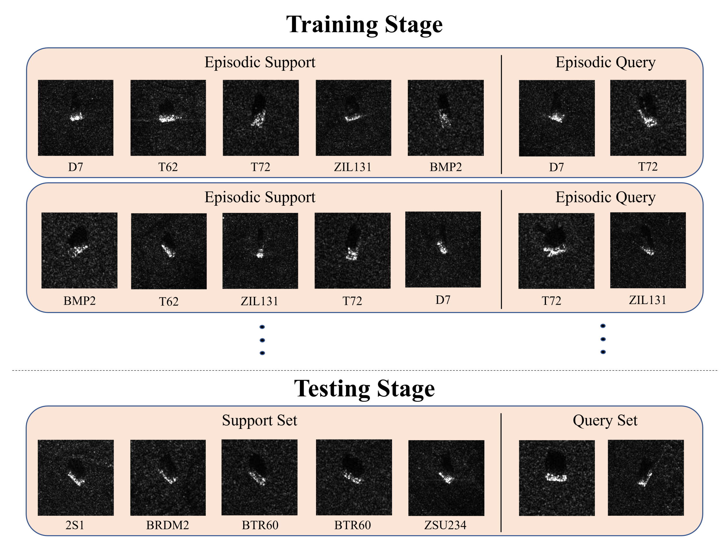
3.1. Problem Definition

In this paper, we follow the common settings of few-shot classification methods. Few-shot classification usually involves a train set and a test set as vanilla classification settings. However, the train set contains base classes $C_{base}$ with a large number of labeled samples. The test set contains different novel classes $C_{novel}$, where $C_{base}\cap C_{novel}=\varnothing$. The test set is further split into the support set, which contains a few annotated samples of the novel classes, and the query set, which contains unlabeled samples of the same label space. Few-shot classification aims to classify the unlabeled query samples given the support set. The few-shot problem is called N-way K-shot if the support set consists of N classes and each class has K labeled samples.

Following previous works, we adopt the episodic training mechanism, as in Figure 2. The episodic training mechanism aims to simulate the test settings in the training stage. In training, we first sample N classes from the $C_{base}$, then sample K images per class from the $C_{base}$ as the episodic support images, and sample Q images per class from the $C_{base}$ as the episodic query images. While in testing, the above sampling process was performed on the $C_{novel}$, and the performance was calculated as the average accuracy over multiple episodes. In our experiments, since there are only 5 classes in $C_{base}$, the classes in every episode are fixed and the only difference lies in the order of the classes. In testing, the support images and the query images are sampled from the $C_{novel}$. Then the probabilities of assigning the query image to the given support class are calculated by their corresponding distance.

3.2. Overall Architecture

The overall architecture of the proposed IAT is shown in Figure 3. IAT mainly consists of three structures: the DCNN backbone for feature extraction based on the input image, a transformer for the feature interaction and refinement, and the distance calculation module to calculate the distances between the query images and the support classes.

The images are first fed into the DCNN backbone to extract features for subsequent stages. After the extraction process of the DCNN backbone, the images are transformed into feature embeddings. Then, the feature embeddings are compressed into a smaller subspace using the shared projection due to efficient consideration.

The transformer is adopted here to model the relationship between the query and support features and strengthen the representation power of all instances. Details will be elaborated in Section 3.3.

The distance calculation module uses a combination of several non-learnable operators to calculate the distances and group the features or distances of the same class. Due to the different purposes, distance calculation modules use separate strategies in training and testing.

As shown in the bottom of Figure 3, in training, to better exploit the representative power of the support instances, the query embedding first calculates distances with all the support instances. The distances of the same class are summed into the specific query-class distance. In testing, to aggregate the information of all the support instances, the support embeddings of the given classes are averaged into the class representations. The distances are calculated between the class representations and the query embedding.

The distances calculated by the above modules are used to infer the predicted class or to calculate loss with the given ground truth.

IAT is trained end-to-end without pretrained weights. IAT follows the episodic training mechanism described in Section 3.1 using the training dataset. The training query and support images are sampled and used to optimize the network. In testing, IAT’s performance is evaluated on the test dataset, in which the data are sampled from the test dataset, which is disjoint from the training dataset.

3.3. Shared Cross-Transformer Module

The transformer used in our paper mainly comprises two parts: the cross attention module and the feedforward network. The cross attention module, as shown in Figure 4a, is responsible for constructing the attention map between query image features and the support image features. The attention module uses support image feature information to optimize the query image features. The cross attention module first transforms the query image features $Q_{in}$ into Q and support image features $S_{in}$ into $K,V$ like Equation (1), where $W_K,W_Q,W_V$ are three learnable matrices to transform the image features into corresponding query, key, and value features.

$$\begin{array}{c}\hfill Q=Q_{in}{W}_Q\\ \hfill K=S_{in}{W}_K\\ \hfill V=S_{in}{W}_V\end{array}$$

(1)

The attention A is calculated using Equation (2), $d_k$ is the dimension of the inputs. The attention module aims to use $K,V$ to optimize Q.

$$A=softmax(\frac{Q{k}^T}{\sqrt{d_k}})$$

(2)

After the attention calculation, Q will update itself using the attention value A and the value vector as Equation (3) and the output feature of Q is called $Q_m$.

$$Q_m=A\left(V{W}_V\right)$$

(3)

The feature $Q_m$ is then refined using a linear layer with parameter $W_O$ and a residual connection to the query image input $Q_{in}$ like Equation (4). The output of $Q_{in}$ after the attention module is $Q_{out}$:

$$Q_{out}=Q_m{W}_O+Q_{in}$$

(4)

When the query image features $Q_{in}$ and the support image features $S_{in}$ are the same, the attention module is called self-attention and we refer the readers to the original transformer paper [25] for more details.

The feedforward network first expands the feature and then squeezes it back to the original dimension using two consecutive linear layers with layer norm and GELU [40] as activation function. The optimization process is described in Equation (5), where $W_1\in {\mathbb{R}}^{d\times d//4},b_1\in {\mathbb{R}}^{d//4},W_2\in {\mathbb{R}}^{d//4\times d4},b_2\in {\mathbb{R}}^d$ denote the parameters of the two linear layers and $\sigma$ is the GeLU nonlinear function.

$$y=\sigma (x{W}_1+b_1)W_2+b_2+x$$

(5)

In the experiments of IAT, the images are transformed into feature embeddings of shape ${\mathbb{R}}^c$. Then, for every query image embedding, it is fed into the transformer with all the support image embeddings. The transformer aims to refine all image features using the attention module and feedforward network. The difference lies in that the query image embedding is not only optimized individually but also aggregated with the support image information based on its similarities to the support image embeddings, while the support image embeddings are only optimized individually by the learned projections.

To better align the features of the query image embeddings and the support image embeddings, several modifications have been made in the vanilla cross-attention module. the detailed structure of the shared cross-attention module is depicted in Figure 4b. The support image embeddings are optimized along with the query image embeddings, and all the projections for the query image embeddings and the support image embeddings are shared to keep them in the same subspace.

In this way, the shared cross-attention optimizes the query image embeddings, such as in Equation (6), and optimizes the support image embeddings, such as in Equation (7), where $q_{in}$ and $s_{in}$ denote the input query and support image embeddings, $q_{out}$ and $s_{out}$ denote the output query and support image embeddings. $W_1$ and $W_2$ are the parameters of the two linear layers.

$$q_{out}=q_{in}+(softmax(\frac{q_{in}{W}_1{\left(s_{in}{W}_1\right)}^T}{\sqrt{d_k}})s_{in}{W}_1)W_o$$

(6)

$$s_{out}=s_{in}+\left(s_{in}{W}_1{W}_2\right)$$

(7)

The optimization of query image embeddings enables them to get an overall understanding of all the support image instances and thus can adapt them based on the estimation distribution of the support classes. The optimization of the support image embeddings can help alleviate the subspace mismatch between the query image embeddings and the support image embeddings.

3.4. DCNN Backbone

The DCNN backbone used in the proposed framework is shown in Figure 5. The backbone, namely, Conv4-64, is commonly used in FSL [32,36], which mainly consists of four convolutional blocks. In each block of the first three layers, there is a convolutional layer with a $3\times 3$ convolution and 64 filters, batch normalization (BN), LeakyReLU, and $2\times 2$ max pooling. The last layer is the same as the previous layers without max pooling.

In our experiment, the input dimension of the backbone is an image of spatial shape $84\times 84$ and the output is flattened into a single feature representation of dimension 1600.

3.5. Loss

For training, the loss function is defined as Equation (8), which mainly follows CAN [23], where the $L_{cls}$ aims to classify all the instances (both the query images and the support images) into their corresponding classes, and the $L_{fs}$ is the few-shot loss, which aims to maximize the similarity of the query image to the correct support class. Both losses are cross-entropy loss and the weight $\lambda$ is set to 0.5.

$$L=L_{cls}+\lambda L_{fs}$$

(8)

The $L_{cls}$ will first predict the probabilities $p_i$ of every instance in the train set using a linear layer. Then cross-entropy loss is adopted based on the ground truth label of the instances.

The $L_{fs}$ is only used in the query samples of the training set, and the ground truth labels of the query samples are generated based on the order of the sampled support classes. The probabilities are calculated by using the softmax function on the query-class distances.

4. Experiments

To evaluate the proposed method, we conducted the experiments as follows. Firstly, some detailed information about our experiments is given in Section 4.1, including a brief description of the used few-shot SAR-ATR dataset, implementation details, and the metric methods for accuracy calculating. Subsequently, the classification results compared with other representative FSL methods are reported in Section 4.2. To verify the effectiveness of the components in the proposed framework, the ablation study was conducted as in Section 4.3, which demonstrates that both the proposed instance cosine distance and the shared cross transformer module contribute to the performance improvement.

4.1. Implementations

4.1.1. Dataset

The Moving and Stationary Target Acquisition and Recognition (MSTAR) dataset [41] (https://www.sdms.afrl.af.mil/index.php?collection=registration, accessed on 7 March 2022), collected by the Sandia National Laboratory SAR sensor platform, is widely used in the studies of SAR ATR to verify different methods’ classification accuracies. The publicly accessible subsets include ten different categories of ground targets (armored personnel carrier: BMP-2, BRDM-2, BTR-60, and BTR-70; tank: T-62, T-72; rocket launcher: 2S1; air defense unit: ZSU-234; truck: ZIL-131; bulldozer: D7). Figure 6 shows the optical images of these targets and the corresponding SAR images. The data were collected using an X-band SAR sensor, in a 0.3 m resolution spotlight mode, with full aspect coverage (in the range of $0^{\circ }$ to ${360}^{\circ }$). Following the general settings in FSL, we randomly selected five categories as the training samples, and only the images acquired under the ${17}^{\circ }$ depression angle were used. Subsequently, the other five categories under the ${17}^{\circ }$ depression angle and ${15}^{\circ }$ depression angle were used as test set 1 and test set 2, respectively.

Table 1. The detailed dataset settings in our experiments. Two test sets were set up to evaluate the performance under different classes and depression angles.

Set	Class	Depression	No. Image
Train	D7	${17}^{\circ }$	299
	T62	${17}^{\circ }$	299
	T72	${17}^{\circ }$	232
	ZIL131	${17}^{\circ }$	299
	BMP2	${17}^{\circ }$	233
Test 1	2S1	${17}^{\circ }$	299
	BRDM2	${17}^{\circ }$	298
	ZSU234	${17}^{\circ }$	299
	BTR60	${17}^{\circ }$	256
	BTR70	${17}^{\circ }$	233
Test 2	2S1	${15}^{\circ }$	274
	BRDM2	${15}^{\circ }$	274
	ZSU234	${15}^{\circ }$	274
	BTR60	${15}^{\circ }$	195
	BTR70	${15}^{\circ }$	196

shows the detailed settings of the training and the test sets.

4.1.2. Implementation Details

For detailed network settings, the DCNN backbone was kept unchanged from the original settings, which are elaborated on in Section 3.4. The output feature dim was 1600, and the shared projection reduced the dimension to 128. The transformer we adopted was a 3 layer, with head 16, dim 128, and the intermediate dimension for the feedforward network was set to 512.

Following previous works, we conducted two experiments for every test set, which were 1 shot and 5 shot. The query image number was set to 15 per class, resulting in a total of 75 query images per episode. Adam was utilized to optimize the network and the learning rate was set to 0.001 for the DCNN backbone and 0.0001 for the transformer. The training episodes were both set to 100. The epoch number was set to 50 and the learning rate decreased by a factor of 10 for every 10 epochs. Our work was built on the LIbFewShot [26] toolbox.

4.1.3. Accuracy Metric

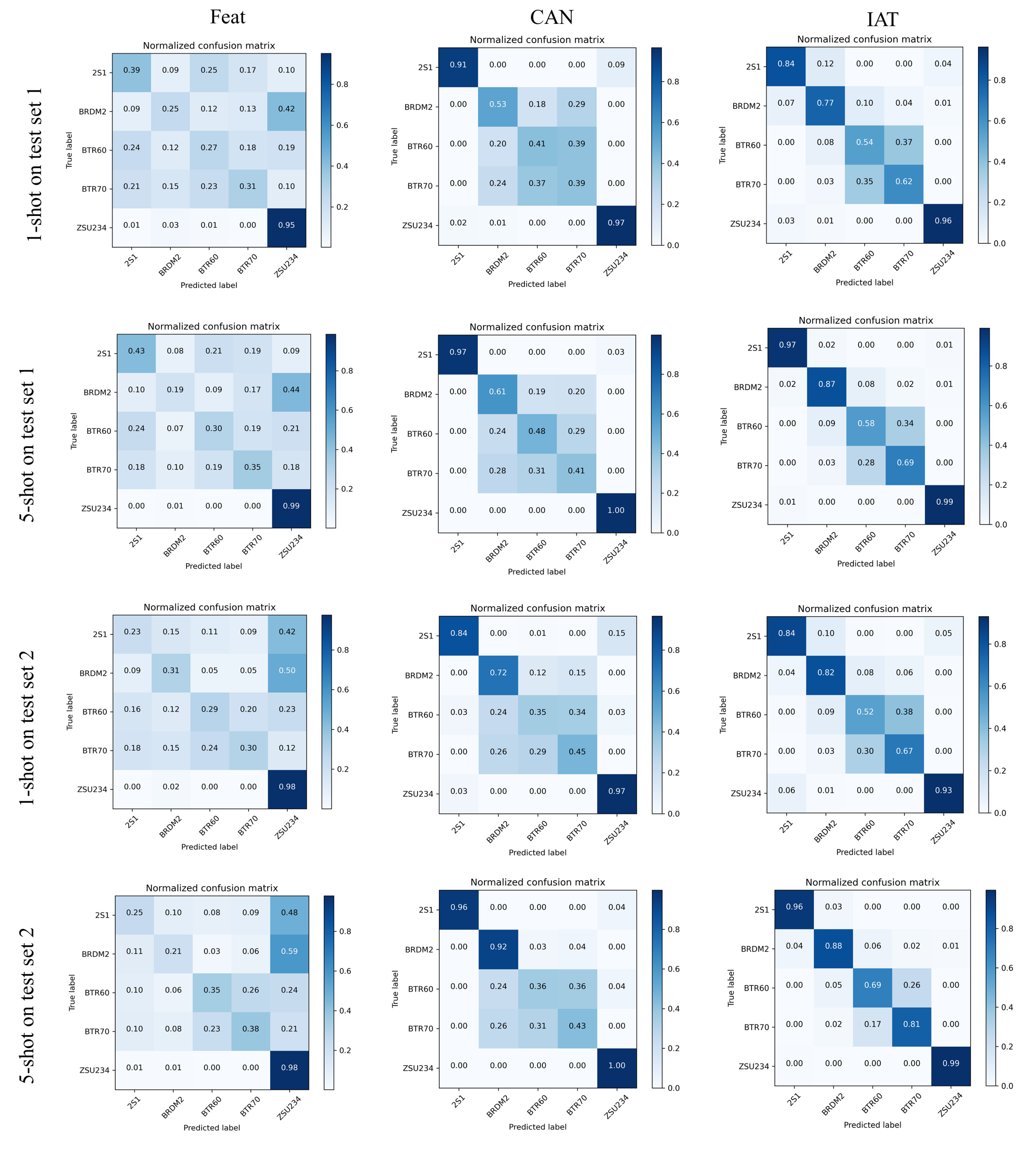
For every episode, the accuracy $AC{C}_i$ was calculated as the ratio of the number of correctly predicted query images to the total number of query images. The detailed calculation process is shown in Equation (9), where the $N_q$ is the total number of query images. $p_i$ and $t_i$ are the predicted class and ground truth class of the i-th query image, and $\mathbb{I}$ is the indicator function, which equals 1 if $p_i=t_i$, else the function equals 0.

$$Ac{c}_i=\frac{1}{N_q}\sum _{j=0}^{N_q}\mathbb{I}(p_i=t_i)$$

(9)

The experiment was repeated multiple times to avoid the effect of randomness and the final accuracy was calculated as the average of all episode accuracies $Ac{c}_i$, as in Equation (10). N in the equation denotes the repeat times of the experiment. In the main experiment, N was set to 600 for all models. In the ablation studies, N was set to 100 for fast inference.

$$Acc=\frac{1}{N}\sum _{j=0}^{N}Ac{c}_i$$

(10)

4.2. Results

The results of IAT on both test sets are reported in

Table 2. Comparison with state-of-the-art methods on the two test sets. Accuracy and 95% confidence interval are presented on the two test sets.

Methods	Test Set 1		Test Set 2
	1 Shot	5 Shot	1 Shot	5 Shot
ProtoNet [36]	${64.349}_{\pm 0.60}$	${78.678}_{\pm 0.43}$	${66.698}_{\pm 0.43}$	${79.640}_{\pm 0.44}$
RelationNet [37]	${55.829}_{\pm 0.61}$	${75.847}_{\pm 0.39}$	${56.256}_{\pm 0.64}$	${76.971}_{\pm 0.37}$
Feat [22]	${43.349}_{\pm 0.46}$	${45.160}_{\pm 0.44}$	${41.922}_{\pm 0.51}$	${43.242}_{\pm 0.42}$
CAN [23]	${64.120}_{\pm 0.52}$	${69.400}_{\pm 0.46}$	${66.544}_{\pm 0.60}$	${73.396}_{\pm 0.35}$
Adm [24]	${69.202}_{\pm 0.56}$	${82.111}_{\pm 0.39}$	${69.387}_{\pm 0.60}$	${84.131}_{\pm 0.36}$
MAML [32]	${55.596}_{\pm 0.68}$	${56.962}_{\pm 0.83}$	${51.658}_{\pm 0.61}$	${58.396}_{\pm 0.74}$
Versa [42]	${56.638}_{\pm 0.60}$	${64.598}_{\pm 0.40}$	${59.127}_{\pm 0.70}$	${64.416}_{\pm 0.43}$
ANIL [43]	${53.760}_{\pm 0.67}$	${70.600}_{\pm 0.54}$	${55.027}_{\pm 0.71}$	${69.944}_{\pm 0.56}$
ConvmNet [44]	${53.167}_{\pm 0.69}$	${62.816}_{\pm 0.62}$	${52.898}_{\pm 0.61}$	${58.956}_{\pm 0.79}$
SKD [45]	${67.996}_{\pm 0.55}$	${81.444}_{\pm 0.39}$	${67.260}_{\pm 0.56}$	${81.924}_{\pm 0.39}$
DN4 [46]	${69.453}_{\pm 0.55}$	${81.091}_{\pm 0.40}$	${70.144}_{\pm 0.64}$	${83.900}_{\pm 0.37}$
IAT	${74.704}_{\pm 0.57}$	${81.913}_{\pm 0.39}$	${75.524}_{\pm 0.69}$	${86.611}_{\pm 0.36}$

. We also provide several few-shot classification method results on the two test sets. IAT outperforms all other works on both test sets. For test set 1, in 1 shot and 5 shot conditions, IAT got an average of 74.704% and 81.913% accuracy, respectively. For test set 2, IAT got an average of 75.524% and 86.611% for the 1 shot and 5 shot classification.

Figure 7 gives the confusion matrixes of Feat [22], CAN [23], and the proposed IAT on both test set 1 and test set 2 under 1 shot and 5 shot conditions. All three models adopted the transformer to refine the features to perform well on the ZSU234 class due to its large difference from other classes, but IAT and CAN can distinguish the 2S1 far better than Feat. The reason why IAT and CAN can effectively improve the classification performance may lie in that Feat only optimizes the support class embedding while IAT and CAN can even refine query embeddings by adopting the shared cross-tansformer module or the cross attention mechanism. Moreover, IAT performs better in recognizing BRDM2 though it is quite similar to the BTR60 and BTR70. IAT’s improvement in discriminating between BTR60 and BTR70 is also clearly presented in the confusion matrix.

4.3. Ablation Studies

In this section, the ablation studies were conducted to analyze the importance of each component in the proposed framework, mainly including the proposed distance calculation method, instance cosine distance, and the shared cross-transformer module. The effectiveness of each component was verified.

4.3.1. Distance Calculation

The distance calculation module transforms the query and support features into the distance between query images and support classes. The distance is used to calculate the loss in training and to infer the query image class in testing. To verify the effectiveness of the proposed different distance calculation settings, several experiments with different settings were conducted. They differ in the choice of the combination of distance calculation methods. We mainly compared the two widely adopted distances (Euclidean and Cosine) with the proposed instance cosine (Ins_cos) distance.

The difference between the instance cosine and the cosine distance lies in that the cosine distance will first average all the support features of the given class, then the distance is calculated between the normalized features. On the contrary, our instance cosine distance fully exploits the instances’ representation by taking the distances of the query image with all the support images into consideration, rather than only using the average feature of the support class. Moreover, instance cosine distance does not normalize the features so the distance can also capture the distance caused by the scale of the features.

The results of using different distance calculations on the two test sets are listed in

Table 3. Performance results of different train-test distance calculation combinations. Bold type indicates the best performance.

Train Setting			Test Setting			Test Set 1		Test Set 2
Ins_Cos	Eucidean	Cosine	Ins_Cos	Eucidean	Cosine	1 Shot	5 Shot	1 Shot	5 Shot
	✓		✓			74.68	76.11	75.95	76.76
	✓			✓		74.68	78.44	75.89	78.75
		✓	✓			64.45	64.20	64.45	65.35
		✓			✓	64.43	69.29	64.43	71.40
✓			✓			75.35	80.99	77.01	83.72
✓				✓		75.28	82.77	76.93	86.91
✓					✓	75.26	82.76	76.96	86.92

. The ✓ in the first column delineates the distance used in the training stage, and the second column delineates the distance used in the testing stage. Other parts were kept the same while comparing the accuracy of different distance calculation methods. When adopting Euclidean or Cosine as the training distance, the best accuracy on test set 1 was 74.68% for 1 shot and 78.44% for 5 shot, and the best accuracy on test set 2 was 75.95% for 1 shot and 78.75% for 5 shot. When adopting instance cosine as the training distance calculation method, the minimum accuracy on test set 1 was 75.26% for 1 shot and 80.99% for 5 shot, and the best accuracy on test set 2 was 76.93% for 1 shot and 83.72% for 5 shot performances, which are all much higher than adopting the other two methods. The experiment’s accuracy demonstrates the superiority of the proposed instance cosine distance in the SAR image few-shot classification.

4.3.2. Shared Cross Transformer Module

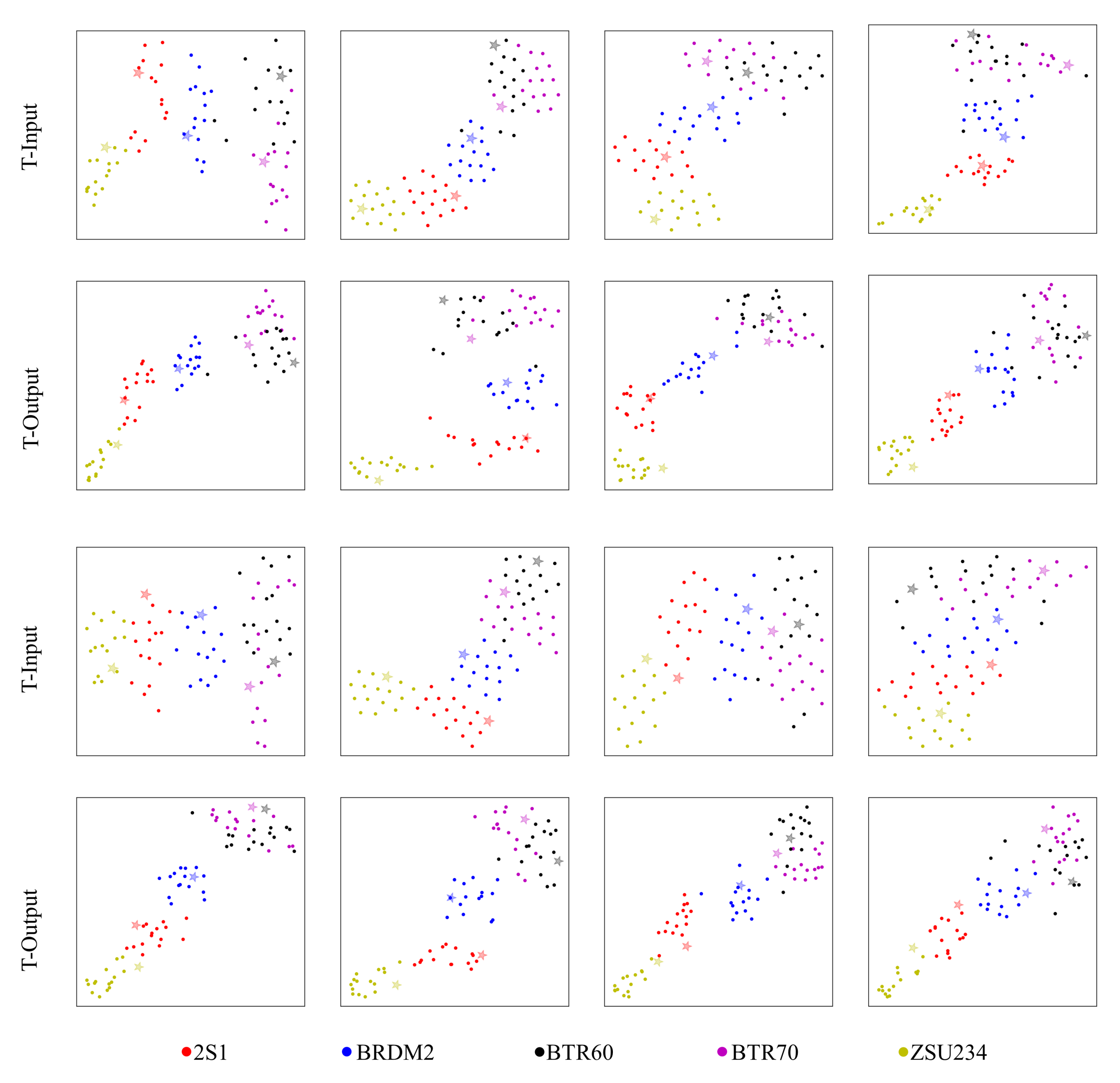
Two main modifications are separated from the shared cross-transformer module to conduct ablation studies of this module. The O-support module optimizes support features along with the query feature, which means support image features will be optimized, as in Equation (7). The S-projection module keeps the query and support features in the same subspace by restricting the projection to be shared, which means that in Equation (1), the projections W are the same.

Results of the different settings are reported in

Table 4. Performance results of different model setting. O-support means optimizing support features along with the query feature, and S-projection means shared projection. Bold type indicates the best performance.

		Test Set 1		Test Set 2
O-Support	S-Projection	1 Shot	5 Shot	1 Shot	5 Shot
		61.44	57.33	63.17	58.60
✓		67.85	76.20	66.89	77.67
	✓	61.29	55.32	59.59	59.51
✓	✓	75.28	82.77	76.93	86.91

. The first experiment adopts neither of the two modules, so it degenerates to the vanilla cross-transformer, as shown in Figure 4a. The second experiment adopts only the O-support; thus, the model optimizes the query and support features using different projections. The third experiment only adopted the S-projection module, in this way, the $W_K,W_V,W_Q$ in Equation (1) were the same, but the support features were kept unchanged during the transformer refinement, which means the transformer only optimizes the query image features. The last experiment was the proposed shared cross-transformer module, which adopted both the O-support and S-projection modules.

When adopting them, the accuracy on test set 1 was 61.44% for 1 shot and 57.33% for 5 shot, and the accuracy on test set 2 was 63.17% for 1 shot and 58.60% for 5 shot. When only adopting the O-support module, the accuracy on test set 1 was 67.85% for 1 shot and 76.20% for 5 shot, and the accuracy on test set 2 was 66.89% for 1 shot and 77.67% for 5 shot. When only adopting the S-projection module, the accuracy on test set 1 was 61.29% for 1 shot and 55.32% for 5 shot, and the accuracy on test set 2 was 59.59% for 1 shot and 59.51% for 5 shot. When adopting both modules, the accuracy on test set 1 was 75.28% for 1 shot and 82.77% for 5 shot, where the accuracy gain was 7.43% and 6.57%. The accuracy on test set 2 was 76.93% for 1 shot and 86.91% for 5 shot, where the accuracy gain was 10.04% and 9.24%. The large accuracy gain on all the test settings shows the importance of simultaneously optimizing both query and support image features and restricting the features in the same subspace.

5. Discussion

The experimental results on the two test sets in Table 2 demonstrate the superiority of our method. IAT outperforms other models in both test sets. In 1 shot settings, IAT achieves 74.704% and 75.524% average accuracy, while the best of other works only got 69.453% and 70.144%. The accuracy increase was +5.251% and +5.38%. The accuracy gains of our model can mostly be attributed to the design of the transformer head since the DCNN backbone was the same in all methods and distance calculation under 1 shot condition was almost equivalent. In 5 shot settings, IAT still performs better than most methods. IAT achieves an average of 81.913% and 86.611% in the two test sets. The experiment results demonstrate the effectiveness of our method, especially under the 1 shot condition.

The confusion matrixes presented in Figure 7 show the accuracy for every test class. Feat and CAN also use the transformer to construct query-support relationships, but the specific usages are different. Feat used transformer to construct the relationship between support classes. Moreover, the transformer only optimizes the support class embeddings, and the query image embeddings are kept unchanged as the output of the backbone, while we optimize both query and support image embeddings. CAN used cross-attention to optimize both the query and support embeddings, and it used the feature map of the query class while we use one dimension embedding, which means IAT focuses more on the global representation of the samples. The results show that IAT can see a consistent performance increase over CAN [23] and Feat [22] in all classes. The accuracy gain shows that IAT’s transformer structure is better at exploiting the support images’ representation power; thus, it benefits the classification of the query images. For the easy class, such as 2S1 and ZSU234, IAT can achieve an accuracy of 0.85 under 1 shot condition and 0.95 under 5 shot conditions. However, the matrixes have also shown that IAT’s performance in discriminating BTR60 and BTR70 is not as outstanding as discriminating others, because the BTR60 and BTR 70 are two similar tanks with almost the same length, width, and height.

Ablation study on the design of the shared cross-transformer module in Table 4 shows the effectiveness of the proposed module. It can be seen that even discarding one of the two modifications, the performance dropped dramatically. The maximum accuracy drop can be up to 20% (from 82.77% to 55.32%). When adopting only one of the two modifications, accuracy on the O-support was far better than in the S-projection, which illustrates the importance of optimizing support features. Optimizing support features without shared projection demands learning two projections, which may result in the support features and query features being in different subspaces. When restricting the projection matrixes to be shared between the query and support features, accuracy increased by +7.43% and +6.57% on test set 1 and +10.04% and +9.24% on test set 2.

The ablation study on different distance calculation methods in Table 3 shows the validity of the proposed instance cosine distance calculation method. When using the Euclidean distance as the training distance, the accuracy under the 1 shot condition was 74.68% and 75.95%, just a little lower than the proposed instance cosine distance. However, under the 5 shot setting, the accuracy was only 78.44% and 78.75%, which was far lower than the proposed instance cosine distance. When using cosine distance as the training distance, the accuracy was the lowest in all settings. This might be due to the loss of scale information introduced by the normalization function, which only considers the angle distance, but abandons the distance introduced by the length of features.

When using instance cosine distance as the training distance, the accuracy can surpass other training settings and the results are relatively stable on different test distance choices. However, when adopting instance cosine distance as the test set, the accuracy on 5 shot is a little lower than adopting other distance methods. The discrepancies exist because of the different purposes of training and testing. In training, IAT aims to refine all the support instances rather than the mutual representation of the class. Therefore, instance cosine distance is adopted to calculate the distance between the query feature and all the support features. In this way, the support features of the correct class were pulled closer to the query feature, instead of just the average features of a support class in Euclidean distance or cosine distance. In testing, however, the goal was to classify the query image into the given support classes (not the support instance), so it is necessary to group the support features into support class representations to enlarge the mutual information from the given sample points. In this paper, we adopted the average of all the support features as the class representation for simplicity and efficiency consideration.

The results also show that when using instance cosine distance as the training set, the performances are nearly the same when using Euclidean or cosine distance as the test set. Such similar performance indicates that the instance cosine distance can satisfy both the distance metric of Euclidean space and cosine space, which proves the superiority of the proposed distance calculation method.

Since all three distance calculation methods do not contain any learnable parameters, replacing the test distance calculation method has no impact on the feature extraction pipeline and the features are determined by the input episodic images and other modules such as the DCNN backbone and transformer head.

To explain the effectiveness of the proposed method more clearly, we utilized t-SNE [47] to visualize the input and output feature of the trained transformer head under both 1 shot (Figure 8) and 5 shot conditions (Figure 9). Figures in the first and third rows indicate the inputs of the transformer (the feature output of the DCNN backbone). Meanwhile, the second and last rows indicate the corresponding outputs of the transformer, respectively. In the figures, asterisks denote the support images, dots denote the query samples, and different colors denote different classes of the images. The model will classify the query images perfectly if the features of query images and support images of the same class are located in a small area of the figure and can be separated easily from other class samples. The features in the input of the transformer head tend to be located continuously across the diagonal of the figure, which will make it hard for the network to correctly classify the samples located in the decision boundary. However, the features after the transformer tend to be clustered together and the distance between different classes is larger, thus making it easier for the network to classify the query samples into the right group. The two figures show that the transformer head can significantly make the query features and the support features of the same category more compact. After the transformer head, both the intra-class compactness and inter-class dispersion are optimized for either the 1 shot setting or 5 shot setting. For specific classes, it can also be deduced that ZSU234 can be classified relatively perfectly even in the input of the transformer and the transformer head can help the discrimination of the other four classes, where the mingled samples are being grouped into their clusters. However, IAT has limited improvement in distinguishing between BTR60 and BTR70, which are concurrent to the result presented by the confusion matrix in Figure 7.

The limitations of our methods were mainly as follows. (1) The accuracy increase under the 5 shot condition was not satisfying, which we conjectured might be due to the optimization problem when the attention map was large, which can be alleviated by regularizing the attention values. The exploration of such regularization methods is left for future works. (2) When facing extremely similar classes like BTR60 and BTR70 in our experiment, IAT still struggles to recognize it. The unsatisfying recognition accuracy may be alleviated by introducing some prior information into the network or adopting some post-processing module. (3) When the support images and query images face large aspect angle variations, it is hard for the network to infer the real classes of the query images since the SAR image changes a lot when the aspect angle changes. Several failure cases are presented in Figure 10.

6. Conclusions

For the purpose of alleviating the performance drop of DCNNs in the data-limited situation, we proposed a novel FSL model named IAT to tackle the few-shot SAR-ATR. By employing transformer to model the query-support relationship and calculate the attention map, the IAT can exploit the power of all instances. In addition, we introduced instance cosine distance in the training procedure of IAT, which calculates the distance between the query image and the support images rather than the query image and the support classes. Such distances can pull all the instances in a given class closer; thus, improving the classification accuracy. Experimental results verify that the proposed IAT is competitive with the state-of-the-art FSL methods. Moreover, the visualization results reveal that the IAT can efficiently improve the intra-class compactness and inter-class dispersion.

References

1. Morgan, D.A. Deep convolutional neural networks for ATR from SAR imagery. In Algorithms for Synthetic Aperture Radar Imagery XXII; International Society for Optics and Photonics: Baltimore, MD, USA, 2015; Volume 9475, p. 94750F. [Google Scholar]
2. Shao, J.; Qu, C.; Li, J. A performance analysis of convolutional neural network models in SAR target recognition. In Proceedings of the 2017 SAR in Big Data Era: Models, Methods and Applications (BIGSARDATA), Beijing, China, 13–14 November 2017; pp. 1–6. [Google Scholar]
3. Chen, S.; Wang, H.; Xu, F.; Jin, Y.Q. Target classification using the deep convolutional networks for SAR images. IEEE Trans. Geosci. Remote Sens. 2016, 54, 4806–4817. [Google Scholar] [CrossRef]
4. Zhang, J.; Xing, M.; Xie, Y. FEC: A feature fusion framework for SAR target recognition based on electromagnetic scattering features and deep CNN features. IEEE Trans. Geosci. Remote Sens. 2020, 59, 2174–2187. [Google Scholar] [CrossRef]
5. Shijie, J.; Ping, W.; Peiyi, J.; Siping, H. Research on data augmentation for image classification based on convolution neural networks. In Proceedings of the 2017 Chinese Automation Congress (CAC), Jinan, China, 20–22 October 2017; pp. 4165–4170. [Google Scholar]
6. Cubuk, E.D.; Zoph, B.; Mane, D.; Vasudevan, V.; Le, Q.V. Autoaugment: Learning augmentation strategies from data. In Proceedings of the IEEE/CVF Conference on Computer Vision and Pattern Recognition, Long Beach, CA, USA, 15–20 June 2019; pp. 113–123. [Google Scholar]
7. Ratner, A.J.; Ehrenberg, H.R.; Hussain, Z.; Dunnmon, J.; Ré, C. Learning to compose domain-specific transformations for data augmentation. Adv. Neural Inf. Process. Syst. 2017, 30, 3239. [Google Scholar] [PubMed]
8. Guo, J.; Lei, B.; Ding, C.; Zhang, Y. Synthetic Aperture Radar Image Synthesis by Using Generative Adversarial Nets. IEEE Geosci. Remote Sens. Lett. 2017, 14, 1111–1115. [Google Scholar] [CrossRef]
9. Goodfellow, I.; Pouget-Abadie, J.; Mirza, M.; Xu, B.; Warde-Farley, D.; Ozair, S.; Courville, A.; Bengio, Y. Generative adversarial networks. Commun. ACM 2020, 63, 139–144. [Google Scholar] [CrossRef]
10. Liu, L.; Pan, Z.; Qiu, X.; Peng, L. SAR target classification with CycleGAN transferred simulated samples. In Proceedings of the IGARSS 2018—2018 IEEE International Geoscience and Remote Sensing Symposium, Valencia, Spain, 22–27 July 2018; pp. 4411–4414. [Google Scholar]
11. Cui, Z.; Zhang, M.; Cao, Z.; Cao, C. Image data augmentation for SAR sensor via generative adversarial nets. IEEE Access 2019, 7, 42255–42268. [Google Scholar] [CrossRef]
12. Cao, C.; Cao, Z.; Cui, Z. LDGAN: A synthetic aperture radar image generation method for automatic target recognition. IEEE Trans. Geosci. Remote Sens. 2019, 58, 3495–3508. [Google Scholar] [CrossRef]
13. Auer, S.J. 3D Synthetic Aperture Radar Simulation for Interpreting Complex Urban Reflection Scenarios. Ph.D. Thesis, Technische Universität München, Munich, Germany, 2011. [Google Scholar]
14. Hammer, H.; Schulz, K. Coherent simulation of SAR images. In Image and Signal Processing for Remote Sensing XV; International Society for Optics and Photonics: Baltimore, MD, USA, 2009; Volume 7477, p. 74771G. [Google Scholar]
15. Malmgren-Hansen, D.; Kusk, A.; Dall, J.; Nielsen, A.A.; Engholm, R.; Skriver, H. Improving SAR automatic target recognition models with transfer learning from simulated data. IEEE Geosci. Remote Sens. Lett. 2017, 14, 1484–1488. [Google Scholar] [CrossRef] [Green Version]
16. Zhong, C.; Mu, X.; He, X.; Wang, J.; Zhu, M. SAR target image classification based on transfer learning and model compression. IEEE Geosci. Remote Sens. Lett. 2018, 16, 412–416. [Google Scholar] [CrossRef]
17. Huang, Z.; Pan, Z.; Lei, B. What, where, and how to transfer in SAR target recognition based on deep CNNs. IEEE Trans. Geosci. Remote Sens. 2019, 58, 2324–2336. [Google Scholar] [CrossRef] [Green Version]
18. Tang, J.; Zhang, F.; Zhou, Y.; Yin, Q.; Hu, W. A fast inference networks for SAR target few-shot learning based on improved siamese networks. In Proceedings of the IGARSS 2019—2019 IEEE International Geoscience and Remote Sensing Symposium, Yokohama, Japan, 28 July–2 August 2019; pp. 1212–1215. [Google Scholar]
19. Lu, D.; Cao, L.; Liu, H. Few-Shot Learning Neural Network for SAR Target Recognition. In Proceedings of the 2019 6th Asia-Pacific Conference on Synthetic Aperture Radar (APSAR), Xiamen, China, 26–29 November 2019; pp. 1–4. [Google Scholar]
20. Wang, L.; Bai, X.; Zhou, F. Few-Shot SAR ATR Based on Conv-BiLSTM Prototypical Networks. In Proceedings of the 2019 6th Asia-Pacific Conference on Synthetic Aperture Radar (APSAR), Xiamen, China, 26–29 November 2019; pp. 1–5. [Google Scholar]
21. Yan, Y.; Sun, J.; Yu, J. Prototype metric network for few-shot radar target recognition. In Proceedings of the IET International Radar Conference (IET IRC 2020), Online, 4–6 November 2020; Volume 2020, pp. 1102–1107. [Google Scholar]
22. Ye, H.J.; Hu, H.; Zhan, D.C.; Sha, F. Few-shot learning via embedding adaptation with set-to-set functions. In Proceedings of the IEEE/CVF Conference on Computer Vision and Pattern Recognition, Seattle, WA, USA, 13–19 June 2020; pp. 8808–8817. [Google Scholar]
23. Hou, R.; Chang, H.; Ma, B.; Shan, S.; Chen, X. Cross attention network for few-shot classification. arXiv 2019, arXiv:1910.07677. [Google Scholar]
24. Li, W.; Wang, L.; Huo, J.; Shi, Y.; Gao, Y.; Luo, J. Asymmetric Distribution Measure for Few-shot Learning. In Proceedings of the Twenty-Ninth International Joint Conference on Artificial Intelligence (IJCAI 2020), Yokohama, Japan, 7–15 January 2020; pp. 2957–2963. [Google Scholar] [CrossRef]
25. Vaswani, A.; Shazeer, N.; Parmar, N.; Uszkoreit, J.; Jones, L.; Gomez, A.N.; Kaiser, L.; Polosukhin, I. Attention Is All You Need. arXiv 2017, arXiv:1706.03762v2. [Google Scholar]
26. Li, W.; Dong, C.; Tian, P.; Qin, T.; Yang, X.; Wang, Z.; Huo, J.; Shi, Y.; Wang, L.; Gao, Y.; et al. LibFewShot: A Comprehensive Library for Few-shot Learning. arXiv 2021, arXiv:2109.04898. [Google Scholar]
27. Chen, W.Y.; Liu, Y.C.; Kira, Z.; Wang, Y.C.F.; Huang, J.B. A closer look at few-shot classification. arXiv 2019, arXiv:1904.04232. [Google Scholar]
28. Dhillon, G.S.; Chaudhari, P.; Ravichandran, A.; Soatto, S. A baseline for few-shot image classification. arXiv 2019, arXiv:1909.02729. [Google Scholar]
29. Yang, S.; Liu, L.; Xu, M. Free lunch for few-shot learning: Distribution calibration. arXiv 2021, arXiv:2101.06395. [Google Scholar]
30. Liu, B.; Cao, Y.; Lin, Y.; Li, Q.; Zhang, Z.; Long, M.; Hu, H. Negative margin matters: Understanding margin in few-shot classification. In European Conference on Computer Vision; Springer: Berlin/Heidelberg, Germany, 2020; pp. 438–455. [Google Scholar]
31. Rusu, A.A.; Rao, D.; Sygnowski, J.; Vinyals, O.; Pascanu, R.; Osindero, S.; Hadsell, R. Meta-learning with latent embedding optimization. arXiv 2018, arXiv:1807.05960. [Google Scholar]
32. Finn, C.; Abbeel, P.; Levine, S. Model-agnostic meta-learning for fast adaptation of deep networks. In Proceedings of the 34th International Conference on Machine Learning (ICML 2017), Sydney, NSW, Australia, 6–11 August 2017; PMLR: Westminster, UK, 2017; pp. 1126–1135. [Google Scholar]
33. Bertinetto, L.; Henriques, J.F.; Torr, P.H.; Vedaldi, A. Meta-learning with differentiable closed-form solvers. arXiv 2018, arXiv:1805.08136. [Google Scholar]
34. Lee, K.; Maji, S.; Ravichandran, A.; Soatto, S. Meta-learning with differentiable convex optimization. In Proceedings of the IEEE/CVF Conference on Computer Vision and Pattern Recognition, Long Beach, CA, USA, 15–20 June 2019; pp. 10657–10665. [Google Scholar]
35. Xu, W.; Wang, H.; Tu, Z. Attentional Constellation Nets for Few-Shot Learning. In Proceedings of the International Conference on Learning Representations, Virtual Event, Austria, 3–7 May 2021; Available online: OpenReview.net (accessed on 7 March 2022).
36. Snell, J.; Swersky, K.; Zemel, R.S. Prototypical networks for few-shot learning. arXiv 2017, arXiv:1703.05175. [Google Scholar]
37. Sung, F.; Yang, Y.; Zhang, L.; Xiang, T.; Torr, P.H.; Hospedales, T.M. Learning to compare: Relation network for few-shot learning. In Proceedings of the IEEE Conference on Computer Vision and Pattern Recognition, Salt Lake City, UT, USA, 18–23 June 2018; pp. 1199–1208. [Google Scholar]
38. Koch, G.; Zemel, R.; Salakhutdinov, R. Siamese neural networks for one-shot image recognition. In Proceedings of the ICML Deep Learning Workshop, Lille, France, 6–11 July 2015; Volume 2. [Google Scholar]
39. Wang, L.; Bai, X.; Gong, C.; Zhou, F. Hybrid Inference Network for Few-Shot SAR Automatic Target Recognition. IEEE Trans. Geosci. Remote Sens. 2021, 59, 9257–9269. [Google Scholar] [CrossRef]
40. Hendrycks, D.; Gimpel, K. Gaussian Error Linear Units (GELUs). arXiv 2020, arXiv:1606.08415. [Google Scholar]
41. Keydel, E.R.; Lee, S.W.; Moore, J.T. MSTAR extended operating conditions: A tutorial. Proc. Spie 1996, 2757, 228–242. [Google Scholar]
42. Gordon, J.; Bronskill, J.; Bauer, M.; Nowozin, S.; Turner, R.E. Meta-Learning Probabilistic Inference for Prediction. In Proceedings of the 7th International Conference on Learning Representations (ICLR 2019), New Orleans, LA, USA, 6–9 May 2019. [Google Scholar]
43. Raghu, A.; Raghu, M.; Bengio, S.; Vinyals, O. Rapid Learning or Feature Reuse? Towards Understanding the Effectiveness of MAML. In Proceedings of the 8th International Conference on Learning Representations (ICLR 2020), Addis Ababa, Ethiopia, 26–30 April 2020. [Google Scholar]
44. Li, W.; Xu, J.; Huo, J.; Wang, L.; Gao, Y.; Luo, J. Distribution Consistency Based Covariance Metric Networks for Few-Shot Learning. In Proceedings of the Thirty-Third AAAI Conference on Artificial Intelligence (AAAI 2019), Honolulu, HI, USA, 27 January–1 February 2019; pp. 8642–8649. [Google Scholar] [CrossRef]
45. Rajasegaran, J.; Khan, S.; Hayat, M.; Khan, F.S.; Shah, M. Self-supervised Knowledge Distillation for Few-shot Learning. arXiv 2020, arXiv:2006.09785. [Google Scholar]
46. Li, W.; Wang, L.; Xu, J.; Huo, J.; Gao, Y.; Luo, J. Revisiting Local Descriptor Based Image-To-Class Measure for Few-Shot Learning. In Proceedings of the IEEE Conference on Computer Vision and Pattern Recognition (CVPR 2019), Long Beach, CA, USA, 16–20 June 2019; pp. 7260–7268. [Google Scholar] [CrossRef] [Green Version]
47. Van der Maaten, L.; Hinton, G. Visualizing data using t-SNE. J. Mach. Learn. Res. 2008, 9, 2579–2605. [Google Scholar]
Figure 1. Illustration of different relation-modeling heads in few-shot field. (a) The support images of the same class are averaged to form the support center and subsequent modules are used to model the relationship between support centers and the query image. (b) Relationships are directly modeled based on all the support images and the query images. To be noted, different colors in the figure indicate different classes.
Remotesensing 14 01884 g001
Figure 2. Episodic training and testing of few-shot classification. The code below each plot indicates its category, which can be found in Section 4.1.1.
Remotesensing 14 01884 g002
Figure 3. The overall architecture of the proposed IAT. The example here is a 2-way k-shot condition.
Remotesensing 14 01884 g003
Figure 4. The proposed shared cross-attention module, where W stands for learnable kernels, different footnotes denote different kernels, and A is the attention matrix. (a) The vanilla setting and extraction pipeline of cross-attention. (b) The pipeline of shared cross-attention module, where query and support features share the same input projection kernel W 1 and output projection kernel W 2 .
Remotesensing 14 01884 g004
Figure 5. Detailed structure of the DCNN backbone. There are mainly four convolutional blocks.
Remotesensing 14 01884 g005
Figure 6. Optical images (top) and SAR images (bottom) for the ten targets in the MSTAR dataset.
Remotesensing 14 01884 g006
Figure 7. Confusion matrixes of Feat, CAN, and IAT on test sets 1 and 2 under 1-shot and 5-shot conditions.
Remotesensing 14 01884 g007
Figure 8. Visualization of the input (the first and third rows) and output features (the second and last rows) of IAT under the 1 shot condition using t-SNE. Asterisks and dots represent the features of support images and query images, respectively. Different colors correspond to different categories.
Remotesensing 14 01884 g008
Figure 9. Visualization of the input features (the first and third rows) and output features (the second and last rows) of IAT under the 5 shot condition using t-SNE. Asterisks and dots represent the features of support images and query images, respectively. Different colors correspond to different categories.
Remotesensing 14 01884 g009
Figure 10. Typical incorrect predictions of IAT under the 1 shot setting. The support images are placed on the left with their corresponding classes. The incorrectly predicted query images are placed on the right and the fonts are in the format of (ground truth class/predicted class).
Remotesensing 14 01884 g010