Spatial and Temporal Inversion of Land Surface Temperature along Coastal Cities in Arid Regions

Abstract

Climate change is undoubtedly affecting the global weather of the Earth. Rapid human civilization has mainly caused this in the last few decades. This research examined the spatial and temporal land surface temperature (LST) in the United Arab Emirates (UAE) coastal cities located in an arid region that faced massive urbanization over the last 50 years. We estimated the LST using by-products of Landsat and MODIS images covering 2000 until 2020. The assessment of LST was performed in two contexts, i.e., spatially and temporally, covering daytime vs. nighttime during the summer and winter seasons. Additionally, a supervised classification technique was adopted to extract the land use and land cover in the study area from the late 1970s until 2018. Unexpectedly, the results indicated that daytime LST in districts near the coastlines (heavily urbanized areas) are lower than the ones far away from the coast (about 9 °C). This observation represents the spatial LST inversion in the study area. Nevertheless, this difference was not observed during nighttime LST temporally, the daytime LST did not increase significantly during either summer or winter seasons. However, the nighttime LST has increased temporally by about 17% since 2000 (the temporal LST inversion). Both LST inversions could be attributed to the uniqueness of the study area, given that bare land desert was replaced by vegetation, high-rise buildings, and industrial activities. Additionally, the wind breeze blowing from the gulf might potentially contribute to cooling the coastal urban area during the daytime. Furthermore, in-depth zonal statistics were conducted to visualize the effect of land use on LST. The study observed that fully built-up areas with vegetation have lower LST than built-up areas without vegetation or a combination of sand and vegetation. The research outcomes are invaluable for decision-makers and researchers in achieving sustainable urban development.

1. Introduction

Many cities worldwide have witnessed rapid urbanization following technological development, prosperity, and population increase. Such an unprecedented change in cities was associated with vital sustainability concerns. As expressed by expanding structures and infrastructures such as buildings and roads, urbanization converts natural land covers (such as sand or vegetation) into built-up and impervious areas [1]. Such impervious surfaces are usually characterized by high thermal conductivity and greater thermal capacity than natural land cover areas [2,3,4]. Moreover, the function of the land use and its intensity could lead to temperature increases depending on the local climate conditions [5]. Heat is stored in impervious surfaces during the day and released during the night [6,7]. Consequently, urban areas tend to experience relatively higher temperatures compared to the surrounding rural areas. This phenomenon is commonly known as the urban heat island (UHI) effect [8]. In other words, the UHI refers to higher near-surface and land surface temperatures in urban areas than in the surrounding rural areas due to urbanization [9,10].

The UHI phenomena are crucial to human and wildlife comfort and can also increase the energy consumption of buildings, the concentration of pollutants, and cause general health problems [11]. In other words, cities will become more vulnerable to sustainable development due to excessive consumption and emissions. Urbanization is usually associated with several adverse environmental effects. For instance, traffic movement, as well as industrial and domestic activities, contribute to releasing higher amounts of greenhouse gases, a situation that increases the influence of climate change and causes a rise in the temporal near-surface temperature of urban centers. Urbanization and climate change contribute to UHI manifestation [12,13,14,15,16]. Note that each land cover type responds differently to the UHI [17,18,19]. Thus, the percentage of various land classes in a study area is essential for UHI studies. The development of a UHI has several effects on thermal conditions and human life quality, where higher temperatures increase energy demand for air conditioning, raise pollution levels, and possibly alter precipitation patterns [20,21,22,23,24]. Consequently, the magnitude and pattern of UHI effects were significant concerns for numerous environmental and climatology studies [25].

The UHI is observed in two forms: land-surface and near-surface UHI [26]. The surface UHI is the temperature difference between the surfaces of urban and surrounding rural areas. This occurrence can be examined using land surface temperature (LST) data retrieved from thermal satellite sensors [27,28]. Conversely, the near-surface UHI is the difference in the near-surface temperature pattern between urban and rural areas. Meteorological data can be used to evaluate near-surface UHI.

The advancement of geographic information science/systems (GIS) and the spectral and temporal resolution of the available satellite images allow researchers to assess the effect of the surface UHI across large areas historically and spatially. Several techniques for image classification using multispectral satellite imagery are available and widely used, such as Landsat and Moderate Resolution Imaging Spectroradiometer (MODIS). The LST measurement changes spatially and temporally, and therefore the LST must be evaluated for different land classes over various time frames for a thorough investigation. The required LST data are usually derived from thermal infrared bands using remote sensing data [29,30,31]. Several studies utilized LST retrieved from a wide range of satellites with different spatial resolutions [32,33,34,35,36,37,38].

Some studies in the literature focused on investigating the LST over arid and semi-arid regions. For instance, Abulibdeh [39] studied the LST over different land-use categories (i.e., urban, green, and bare areas) in eight cities that are located in arid and semi-arid regions. Those cities are (i) Doha in Qatar, (ii) Abu Dhabi, (iii) Dubai in the United Arab Emirates (UAE), (iv) Riyadh, (v) Jeddah in Saudi Arabia, (vi) Muscat in the Sultanate of Oman, (vii) Kuwait City in Kuwait, and (viii) Manamah in the Kingdom of Bahrain. The results indicate that bare areas had the highest mean LST values than urban and green areas, with an average increase of 1 to 7 °C. The author also emphasized some fluctuations in the LST analysis among land use categories, which means that a specific land use category may not always have higher or lower LST compared to other categories. Another work by Mohamed et al. [40] studied the LST during the winter and summer seasons in Makkah city in Saudi Arabia. They analyzed the LST over two districts with different built-up materials, i.e., organic vs. deformed iron grids with fragmented paralleled street networks. Their results show that the latter was higher by 1–1.5 °C than the other district. Further, they showed that zones currently under construction had a relatively higher LST than residential zones. A study by Bala et al. [41] established a model to estimate the LST during the day and night in two semi-arid cities (i.e., Ahmedabad and Gandhinagar in India) at different seasons. Their model included variables that are: the normalized difference vegetation index (NDVI), normalized difference built-up index (NDBI), the impervious surface fraction (ISF), and land cover. The R² values of the developed models (day vs. night in different cities) ranged from 0.63 to 0.81.

Interestingly, several studies have investigated the influence of specific meteorological conditions on mitigating UHI or LST. The specific conditions could include cloud or fog formations, haze, precipitation, wind, and others [42]. In arid and semi-arid regions, the wind is the most probable meteorological condition on the above list. Generally, cool winds mixed with hot air over urban areas would yield cooler urban areas. However, the mitigation effect of the wind depends on several factors, including wind speed, direction, and source. For instance, the sea breeze could carry water vapors that might impose greater leverage in mitigating UHI. One study has shown that UHI could be completely mitigated if wind speed reached a specific threshold (depending on the type and size of the urban area) [5]. The study has shown that the larger the urban population is, the higher the wind speed threshold. Sakakibara and Matsui [43] investigated the effect of wind on the UHI phenomenon in coastal cities in Japan. They found that coastal cities that received sea breeze with lower temperatures had a less severe UHI effect than other cities far from the coastlines. Another study by Zak et al. [44] investigated the UHI effect in two big cities in Europe, i.e., Prague and Bucharest. The authors found that UHI is more intense in Bucharest than in Prague, where the intense anticyclonic conditions with winds amplified the intensity. Other studies illustrated how wind could mitigate the UHI effect, such as [45,46,47].

Although several studies investigated and modeled the UHI phenomenon with respect to land cover and land use [48,49,50,51], few studies have conducted a comprehensive analysis of LST in spatial and temporal contexts. For example, is the LST in day and night changing over the years? Additionally, what is the effect of the proximity to the coast in LST? What is the impact of transforming desert bare lands into vegetation? These are critical areas that require careful consideration and would provide invaluable insights to urban planners and decision-makers, among others. Moreover, most of the study areas of those articles had an urban development from vegetation to built-up lands, which resulted in the conventional UHI phenomenon. However, what if the study area transforms from bare lands (sands) into a modern urban system, including high-rise buildings and vegetation areas?

The UAE is one of the countries that has witnessed massive urbanization since the early 1970s. The expansion in the UAE was not limited to urban development but was also extended to population increase and the associated changes in people’s lifestyles. The UAE is a semi-arid region with limited freshwater resources and minimal precipitation. The main cities in the northern emirates of the UAE, such as Dubai, have expanded by approximately five times since 1970 [48]. Some studies revealed that the UHI in arid regions such as the UAE could be inversely relative to regions with other climate types [8].

The main goal of this study is to explore and investigate the LST in the northern UAE, given the rapid urbanization that transpired there in the last few decades. The significance of this study lies in studying how the LST is changing temporally and spatially in a unique environment, i.e., a harsh arid climate with fast-paced urbanization that transformed the bare desert into buildings, roads, and vegetation. Additionally, and unlike many other studies in the literature, we will be investigating the effect of proximity to the coast on LST changes. The assessment of how LST changed in our study area will provide a better understanding of how to mitigate the UHI in the future design of the urban regions, where this could be applicable in the spatial and temporal contexts alike. The specific objectives of this research are to:

• Assess the land cover change in the study area, including built-up areas, water bodies, vegetation, and desert areas for the last five decades (1976–2017);
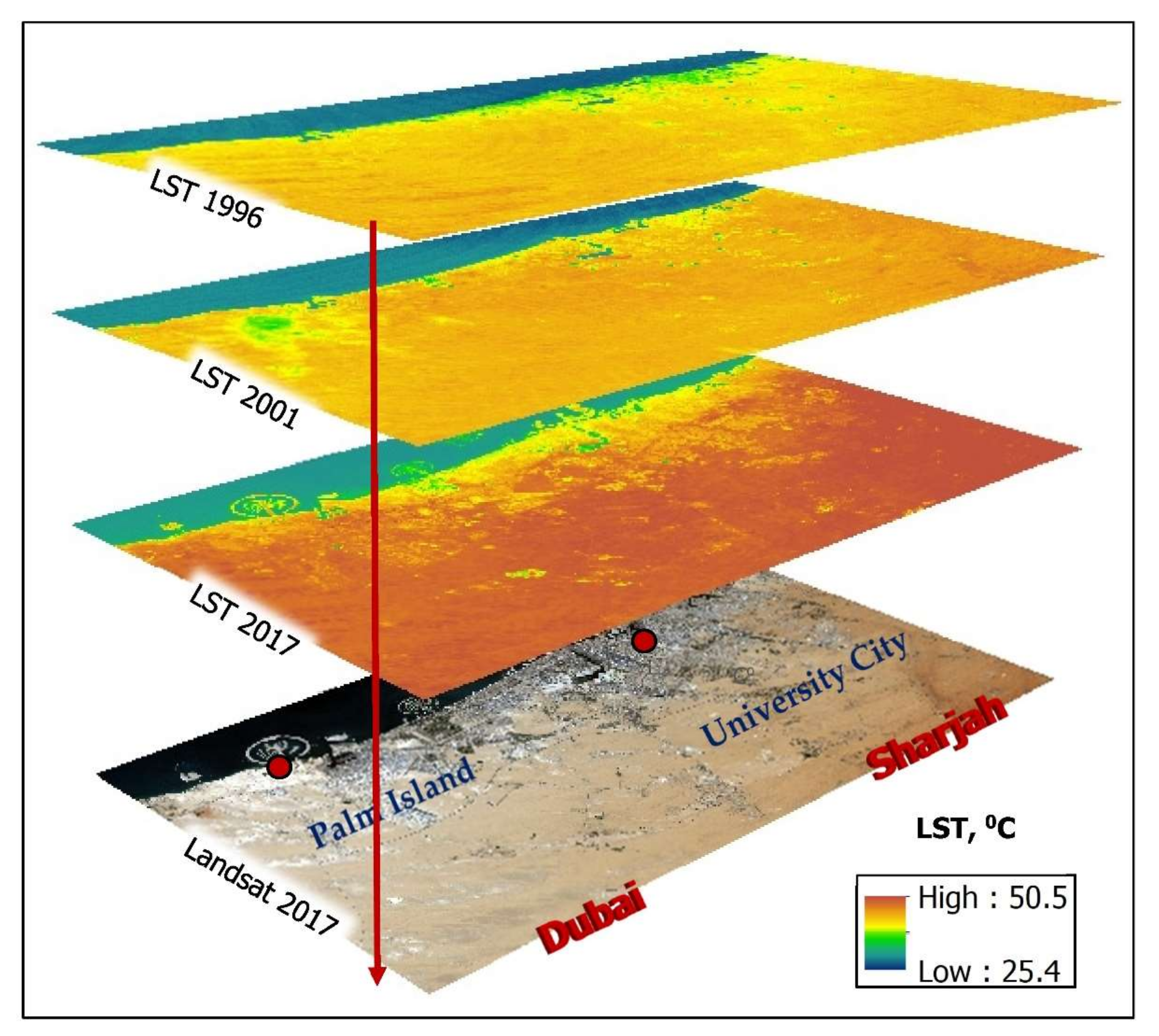
• Understand how the LST changed spatially and temporally in the study area;
• Examine the changes of LST between daytime and nighttime in the summer and winter seasons.

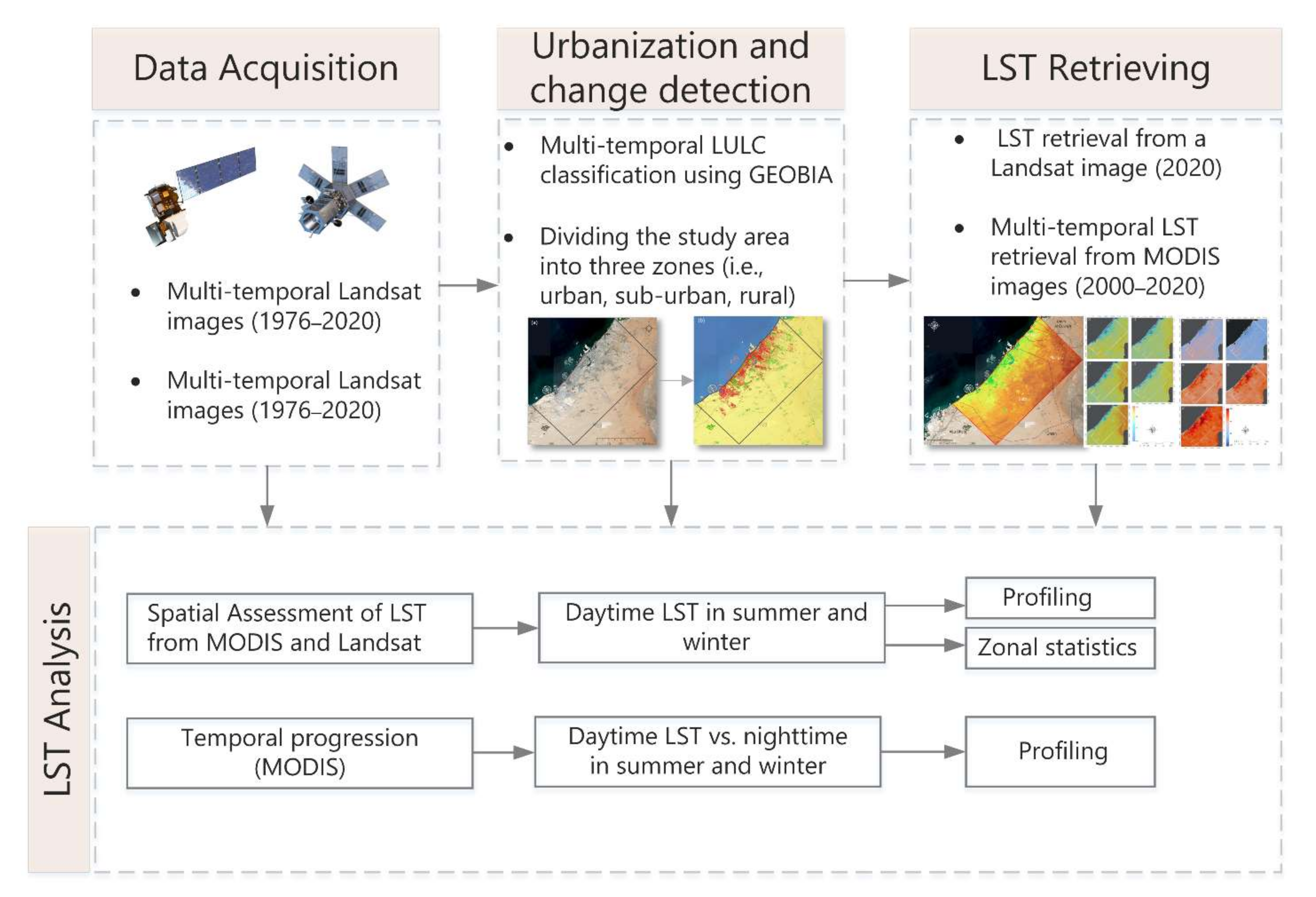
2. Methodology Framework

As illustrated in Figure 1, the methodology framework in this research consists of four main phases. In phase one, numerous satellite images were collected from Landsat, MODIS, and Sentinel-2 satellites to capture the long-term changes across the study area.

In phase two, we examined the urban sprawl pattern across the study area with respect to built-up areas, desert areas, vegetation, and water bodies. This approach allowed us to correlate the calculated LST over urbanized areas and compare the values to virgin desert areas. Additionally, we divided the study area into different zones according to their proximity to coastal lines and urban development (i.e., urban and rural areas). This step was crucial for better investigating how the LST has changed over the years with respect to factors such as urbanization, temperature variations over time, and closeness to the coastline.

We calculated the LST for the study area at phase three, given Landsat and MODIS images. We compared the LST with the near-surface temperature recorded at two airport stations in the study area just before the final stage. Moreover, we analyzed the temporal changes in the near-surface temperature over five decades. This comparison is interesting and gives the manuscript depth concerning the difference between LST and near-surface temperature. Further, we investigated the wind pattern of the study area concerning wind speed, direction, and frequency. As discussed earlier, the wind could have an effect on mitigating the UHI phenomenon. Therefore, understanding the wind pattern could help in explaining observations related to LST.

We examined the LST in the study area spatially and temporally at the final stage. We are dependent mainly on Landsat images, given their relatively higher spatial resolution for the spatial context. However, we compared them with the LST from MODIS images. Five profiles covering the study area were exploited to visualize how the LST is changing spatially during summer and winter (only for daytime). Furthermore, we conducted a low-level analysis using zonal statistics for selected areas within the study area that have unique land use. For the temporal context, we depended on the LST out of MODIS images only, given their relatively higher temporal resolution. The same profiles that were used to assess the spatial changes of LST were used in this part, but the temporal assessment covered daytime vs. nighttime in summer and winter seasons alike.

3. Data Acquisition

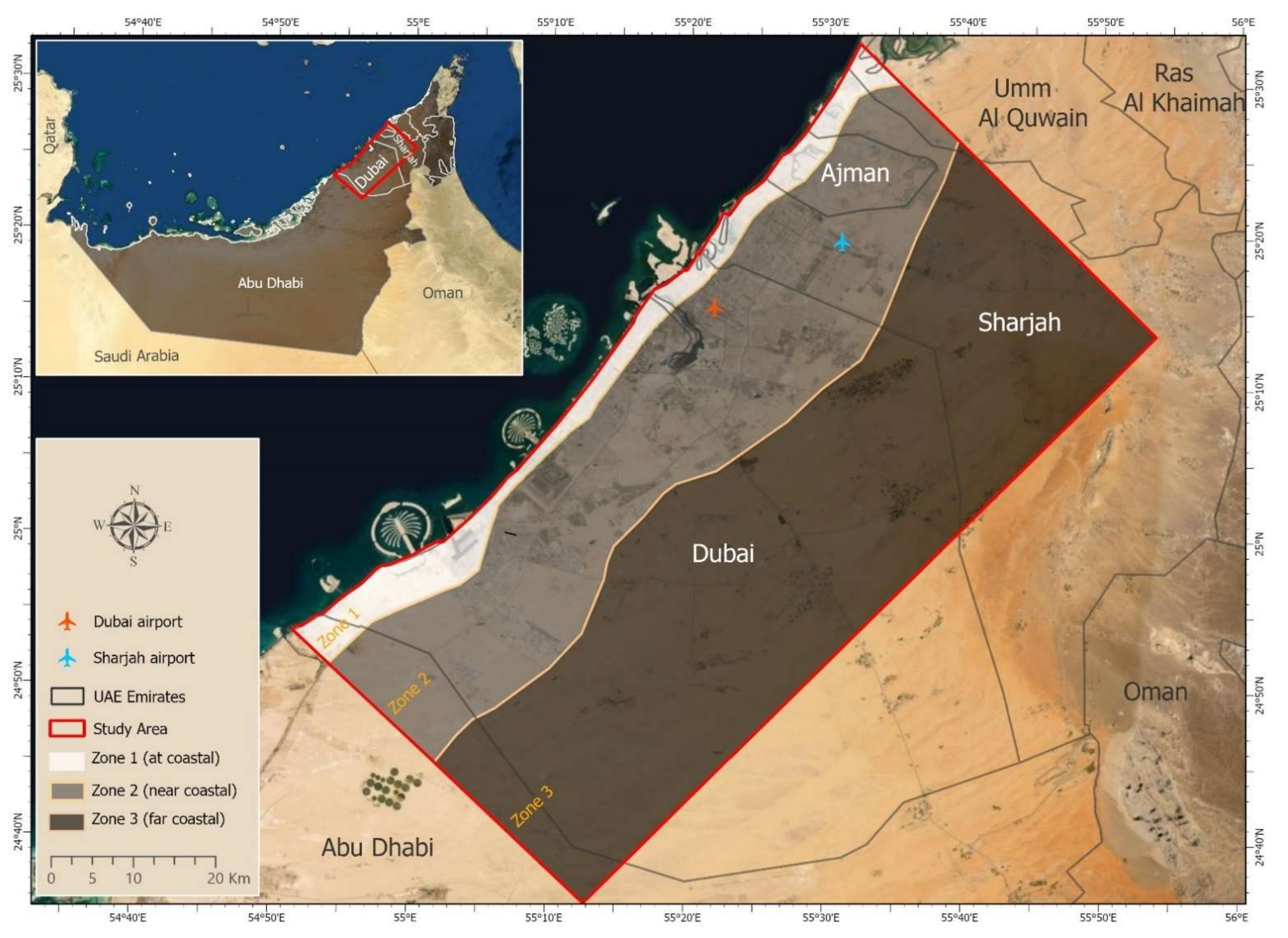
3.1. Study Area

The coastal areas of the UAE were considered for UHI analysis. The study area includes the cities of Dubai, Sharjah, and Ajman (Figure 2). Dubai is the business capital of the UAE and its largest city. Dubai is approximately 4100 km², with a population of more than 3 million [49]. On the other hand, Sharjah is the cultural and industrial capital of the UAE. With over 1.5 million residents over an area of approximately 230 km², Sharjah has the highest population density in the UAE [50]. Finally, Ajman is the smallest emirate in the UAE but has a fast-growing economy with a high demographical evolution [51]. As illustrated in Figure 2, the study area is divided into three zones: at-coastal (distance from the coast is about 2.5 km), near-coastal (distance from the coast is about 20 km), and far-coastal zones (distance from the coast is about 46 km). This division was achieved according to two criteria. The first criterion is related to the proximity of the area to the coast, and the second one pertains to urban development status (urban versus rural areas). However, it is essential to mention that the division was not based on a quantitative measure but rather on the subjective estimation of the proximity distance, as well as our expert opinion about the study area.

Since the establishment of the UAE in 1971, the country (in general) and the study area (in particular) have experienced rapid urbanization and industrialization because of oil discovery and the urban planning policies of its leadership. In Dubai, Khalil et al. [48] studied the city’s urban sprawl from the early 1970s until 2015. They showed that urbanization and population increased dramatically by 5- and 12-fold, respectively. In Sharjah, Al-Ruzouq et al. [50] performed a change detection of the built-up area in the city. They confirmed that the urbanization area of Sharjah almost quadrupled during 1976–2016. Al-Ruzouq et al. [51] investigated the urban growth in Ajman. Their results indicated the urban areas in Ajman increased by approximately 12-fold from 1975 to 2015. Generally, the selected study area is one of the fastest-growing regions with one of the highest urbanization rates in the world.

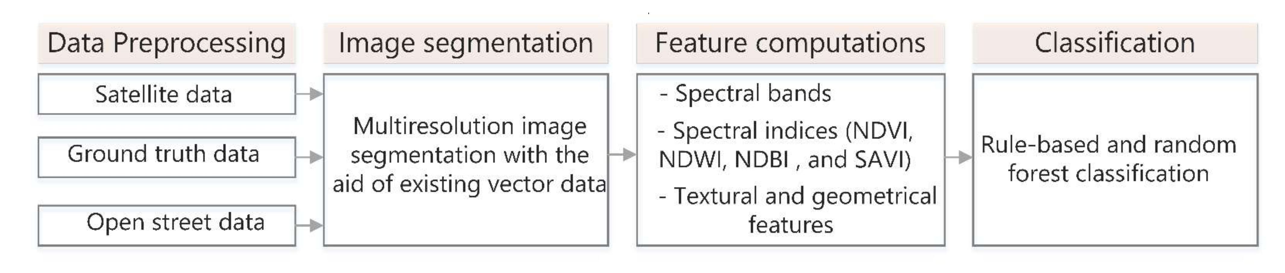
3.2. Data Processing

As mentioned, images from multiple Landsat satellite versions (Landsat 1 to 8), MODIS, and Sentinel-2 were collected to achieve the objectives of this study. The Landsat was used for urban change detection and LST assessment, MODIS for LST assessment, and Sentinel-2 for urban change detection.

It is important to highlight that multiple satellite images were collected to calculate the average LST over each year’s summer and winter seasons. For instance, the summer period was represented by the average LST of the month of August, whereas the winter period was represented by January. This approach helped in minimizing the potential influence of possible unusual meteorological conditions on single dates, such as cloud or fog formation. Moreover, the study area is in a semi-arid region where cloud formation rarely happens.

The thermal images of Landsat and MODIS were taken as an average of selected periods to represent the summer and winter seasons. This approach allowed us to capture a representative LST while avoiding extraordinary meteorological conditions that might occur on certain dates. The number of thermal bands varies from one satellite version to another, and more imaging options were added to higher Landsat satellite versions. For example, no thermal bands were presented in Landsat 1–3, one thermal band was available in Landsat 4–5 (TM) and Landsat 7 (ETM+), and two thermal bands were present for Landsat 8. Interested readers may refer to these articles for further details about the thermal bands of the Landsat satellite [52,53,54]. The Landsat satellite crosses the equator at 10:30 a.m., allowing for LST mapping during the daytime. Therefore, daytime acquisitions are considered to be operational acquisitions. However, nighttime acquisitions are available but require approval.

On the other hand, MODIS captures daily images for the daytime and nighttime but with a lower resolution compared to Landsat. Therefore, Landsat imagery data were used for land classification as well as LST derivation for spatial assessment. The MODIS images were used for the temporal LST assessment. The Landsat images were collected only for the summer seasons from 1976 until 2017 for land classification and 2020 for the LST assessment. The MODIS, on the other hand, was collected for summer and winter, daytime and nighttime, for the period between 2000 and 2020 (every five years).

4. Urbanization and Change Detection

This study employed supervised image classification techniques to detect the urban sprawl in the study area, namely the geographic object-based image analysis (GEOBIA). Areas were classified into built-up, desert, vegetation, and water bodies according to their land use. The adopted GEOBIA classification framework comprises four main steps, as shown in Figure 3.

First, preprocessing multitemporal remotely sensed data, including radiometric and atmospheric corrections, mosaic generation, and the subset of the study area, was carried out. Second, image object generation using a multiresolution image segmentation algorithm was performed using eCognition Developer software. The parameters of the image segmentation algorithm, such as scale, shape, and compactness, were set to 100, 0.5, and 0.1, respectively. The quality of image segmentation could highly impact the accuracy of the succeeding feature computation and classification results [55,56]. The existing and open street vector data were incorporated into the image segmentation to improve image segmentation quality. Third, feature computations and selection were carried out. A set of spectral indices, geometrical and textural features, were computed from the image objects for further analysis [57,58,59,60]. Some of the utilized spectral indices include the normalized difference vegetation index (NDVI) [61], normalized difference water index (NDWI) [62], normalized difference building index (NDBI) [63], and soil adjusted vegetation index (SAVI) [64]. Classification of image objects was carried out using a combination of rule-based and random forest classification approaches. The classification result was evaluated by deriving the standard confusion matrix, as shown in

Table 1. Confusion matrix of the utilized GEOBIA classification approach.

Class	Bare Soil	Water Bodies	Built-Up Areas	Vegetation	Total	User’s Accuracy
Bare soil	116	0	16	0	132	0.88
Water bodies	1	124	0	0	125	0.99
Built-up areas	18	0	106	0	124	0.85
Vegetation	4	4	2	109	119	0.92
Total	139	128	124	109	500	0.00
Producer’s Accuracy	0.83	0.97	0.85	1.00	0.00	0.91

. The overall accuracy and Kappa coefficient achieved by the GEOBIA approach were 91% and 0.88, respectively. Figure 4 depicts the classification result of the most recent satellite image using the GEOBIA technique.

Figure 5 shows the assessment of the temporal built-up increase across the study area divided into three predefined zones: at-coastal, near-coastal, and far-coastal sections. The at-coastal zone was the most urbanized zone compared to other zones. In 2017, the urbanization of the at-coastal zone matched that of the near-coastal zone, with both scoring an urbanization rate of 59% of their built-up area (notice the trend within the shaded box in Figure 5). This outcome shows that the rate of urbanization in the near-coastal zone was faster than that of the at-coastal zone. The reason behind this circumstance is that urbanization started earlier in the at-coastal and near-coastal zones as compared to that in the far-coastal zone. The far-coastal zone had the lowest urbanization rate and percentage of built-up area. In 1976, the far-coastal zone was a bare desert with zero percent urbanization.

5. LST Retrieving from Satellite Images

As mentioned earlier, the spatial assessment of the LST depended on Landsat satellite images. Retrieving LST maps involves the usage of thermal bands to generate a surface temperature map for the study area. This section explores the retrieval of LST.

The Landsat-8 satellite consists of two science instruments that include two sensors: OLI with bands 1 to 9 and TIRS with bands 10. Landsat-8 thermal bands are used to estimate the LST using the following steps:

• Step 1: Convert the digital number (DN) to the top of atmosphere (TOA) radiance value;

$${\mathrm{L}}_{\mathsf{\lambda }}={\mathrm{M}}_{\mathrm{L}}\times {\mathrm{Q}}_{\mathrm{L}}+{\mathrm{A}}_{\mathrm{L}}$$

(1)

where:

• L_λ: top of atmosphere (TOA) radiance value (W/(m² sr μm));
• M_L: band-specific multiplicative rescaling factor;
• A_L: band-specific additive rescaling factor; and
• Q_cal: quantized and calibrated standard product pixel values (DN of bands 10 and 11).

Then, convert the TOA values to TOA brightness temperature (microwave radiation traveling from the top of the atmosphere) in Kelvin:

$$\mathrm{BT}=\frac{{\mathrm{K}}_2}{{\mathrm{L}}_{\mathrm{n}}\times \left(\frac{{\mathrm{K}}_1}{{\mathrm{L}}_{\mathsf{\lambda }}}+1\right)}$$

(2)

where:

• BT: TOA brightness temperature (Kelvin);
• L_λ: TOA spectral radiance (W/(m² sr μm));
• K₁: band-specific thermal conversion constants (W/(m² sr μm));
• K₂: band-specific thermal conversion constant (Kelvin); and
• L_n: the natural logarithm.

Afterward, convert the brightness temperature in Kelvin to Celsius using Equation (3):

$$\mathrm{BT} \left(\mathrm{Celsius}\right)=\mathrm{BT}\left(\mathrm{Kelvin}\right)-273$$

(3)

Subsequently, the derivation of land surface emissivity could be calculated as follows:

$$\mathrm{LES}=0.004\times {\mathrm{P}}_{\mathrm{v}}+0.986$$

(4)

$${\mathrm{P}}_{\mathrm{v}}={\left(\frac{\mathrm{NDVI}-{\mathrm{NDVI}}_{\min }}{{\mathrm{NDVI}}_{\max }-{\mathrm{NDVI}}_{\min }}\right)}^2$$

(5)

where:

• LSE: land surface emissivity;
• P_V: proportion of vegetation; and
• NDVI: normalized difference vegetation index.

To calculate the LST, the following equation is employed:

$$\mathrm{LST}=\frac{\mathrm{BT}}{\left(1+\left[\frac{\mathsf{\lambda }\times \mathrm{BT}}{\mathrm{p}}\times \ln \left(\mathrm{LSE}\right)\right]\right)}$$

(6)

where:

• LST: land surface temperature (Celsius);
• BT: TOA brightness temperature (Celsius); and
• λ: wavelength of emitted radiance (10.60 to 12.51 µm of bands 10 and 11).
• p is calculated using Equation (7).

$$\mathrm{p}=\mathrm{h} \times \frac{\mathrm{c}}{\mathrm{s}}$$

(7)

where:

• h: Planck’s constant (6.626 × 10⁻³⁴ Js);
• s: Boltzmann constant (1.380 × 10⁻²³ J/K); and
• c: velocity of light (2.998 × 10⁸ m/s).

The mono-window algorithm was applied to retrieve the LST maps for the study area by considering the various time frames introduced earlier.

• Step 2: Convert the spectral radiance to the brightness temperature (BT);
• Step 3: Calculate the emissivity and generate the NDVI;
• Step 4: Retrieve the LST maps.

We utilized the methodology proposed by Ermida et al. [65] to retrieve LST from Landsat images through the Google Earth Engine (GEE) platform to facilitate the process. Interested readers could visit this reference for more details [65].

The other source of the LST was the Moderate Resolution Imaging Spectroradiometer (MODIS). The MDOIS Terra (MOD11A1.006) provides daily LST with a resolution of 1000 m for daytime as well as nighttime. The values of the temperature are derived from the “MOD11_L2” swath product. To facilitate the process of retrieving data, we utilized the GEE to specify to download MODIS LST data. Figure 6 shows the average LST of August from 2000 until 2020 at a five-year interval. As can be seen, the LST seems to be slightly increasing in some areas (refer to the illustrated shaded box as an example). We are implementing the same five profiles mentioned before to better understand how the LST changed temporally over our study area. Similarly, we examined how the night LST is changing temporally. Figure 7 shows the temporal nigh time LST over our study area. Generally, and as can be seen, the LST at nighttime has increased over the years. The highest LST increase appears to happen in the far coastal areas close to the land bare sand. Figure 8 presents a 3D integration of the temporal LST maps with the true color Landsat image of the study area in 2017. The temporal pattern of LST and its relation to urbanization, climate change, and closeness to the coast will be discussed in the coming sections.

6. Near-Surface Temperature versus LST

To proceed further with the analysis, assessment and validation were conducted to examine the temporal change in near-surface temperature since the early 1970s. Then, a comparison between LST and the near-surface temperature was made to test the consistency of temperature at the selected dates during the peak summer period (15 July to 5 August).

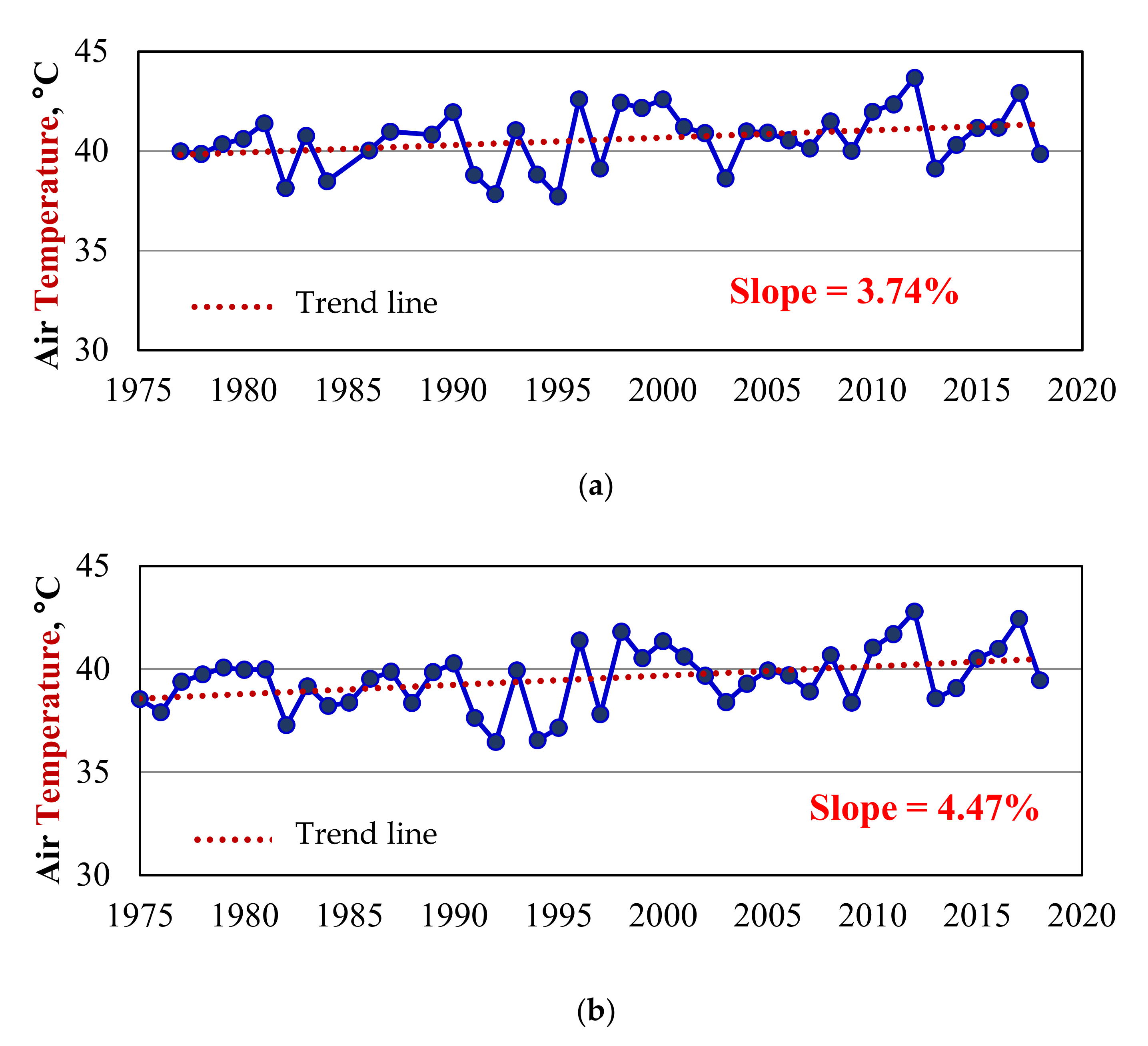
6.1. Temporal Variations of Near-Surface Temperature since the 1970s

Exploring how the near-surface temperature changed during the last five decades is important to illustrate the changes in the LST. The last five decades in the UAE have witnessed an economic and development boom following the oil discovery that resulted in the urbanization sprawl. The UAE community changed from distant villages into modern dense metropolitan cities with many megastructures and modern infrastructure. Of course, this development had side effects on the local environment, and one of these effects is the changes in LST and near-surface temperature. Figure 9 summarizes the temporal annual near-surface temperature retrieved from weather stations located at two major airports in the study area, i.e., Dubai International Airport and Sharjah International Airport (Figure 2). To account for the selected dates of the LST maps at the passing time of the Landsat satellite, the average temperature was taken at 11:00 a.m. from 15 July to 5 August. In Figure 9a, one can observe that there is an increasing trend in the near-surface temperature at Sharjah International Airport at a rate of 3.74%, which can be translated to 0.37 °C every ten years. On the other hand, the near-surface temperature at Dubai International Airport’s weather station shows an increase of 4.47%, which is equivalent to 0.47 °C every ten years (Figure 9b). Hence, the study area has experienced a rise in the near-surface temperature similar to other regions in the world (because of the climate change effect). This increase is expected to affect the LST by default and the UHI phenomena in the study area. This temperature increase was tested using the t-test. For the records of Sharjah airport, the temperature of the summer of 1980 was compared with the records of the summer of 2018 using the t-test. The resulted p-value shows a statistical significance of 99% with a p-value < 1).

6.2. Quantitative Comparision of Near-Surface Temperature and LST

To assess and validate the accuracy of the retrieved LST maps, a comparison between LST and the near-surface temperature was conducted in two selected areas, i.e., the weather station of Sharjah International Airport and Dubai International Airport (Figure 2). Figure 10 shows the temperature difference between the LST at Sharjah and Dubai Airports’ weather stations and the actual temperature retrieved from these stations. As expected, the LST is always higher than the near-surface temperature. Nevertheless, the temperature difference was not consistent at the two locations. This observation was also indicated in the literature as other studies found that the temporal contrast of near-surface temperature and LST is not necessarily consistent [66]. The maximum difference scored was at Sharjah Airport in 2017 with a temperature difference of about 5 °C. On the other hand, the minimum difference was also at Sharjah Airport in 1996, with a temperature difference of about 0.5 °C. The mean difference between the LST and near-surface temperature of both airports over the years is 2.89 °C. It is essential to mention that previous studies for the same region indicated a strong correlation between the LST and near-surface temperature, reaching 0.9 [67].

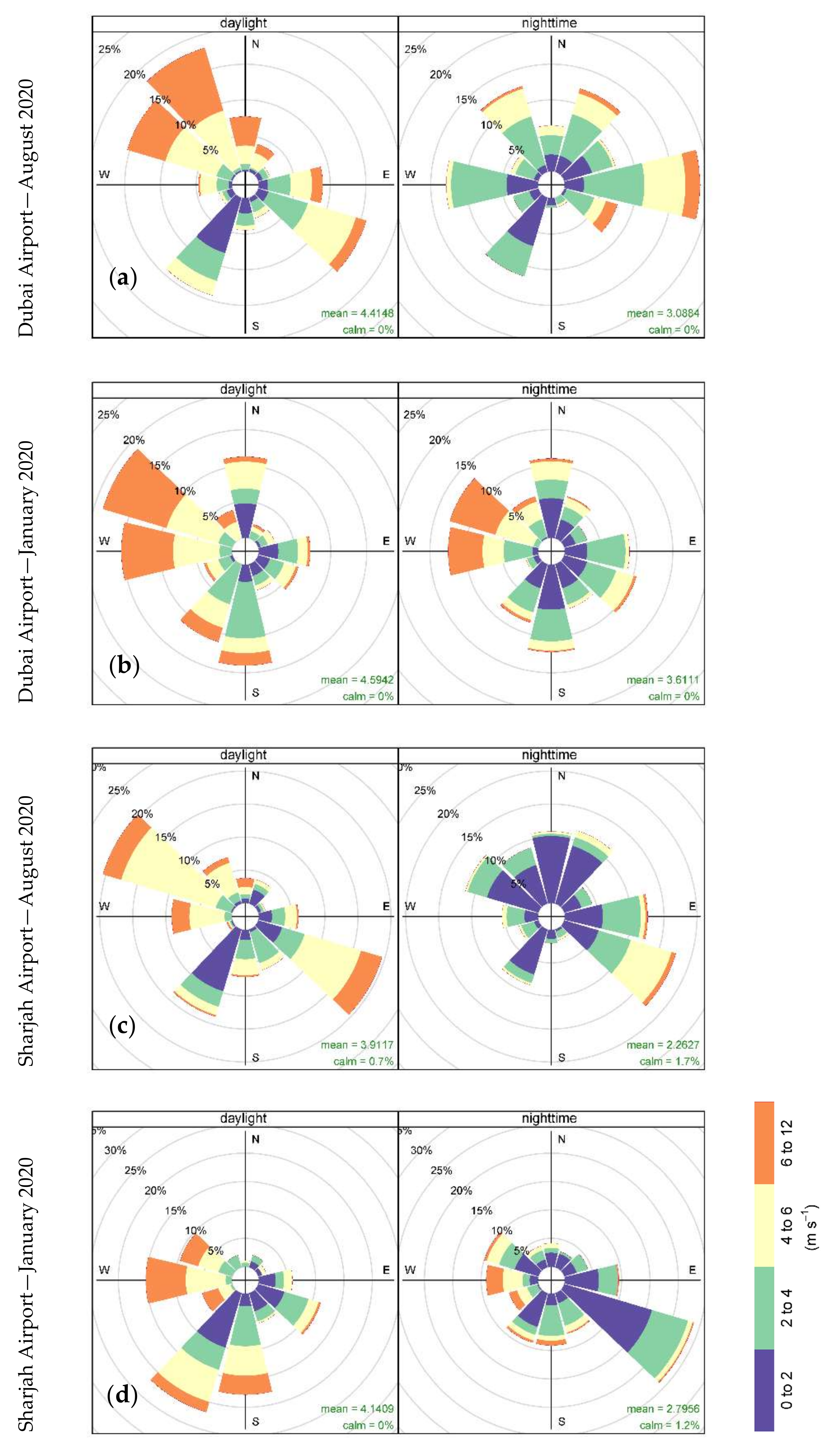
7. Wind Pattern Analysis

To assess the wind pattern in the study area, we were able to collect data related to two airport stations, as shown in Figure 2. Two time periods were considered for the wind analysis, i.e., daytime and nighttime, where all investigations are conducted for 2020. There are many available styles and methods to assess a wind pattern in any study area. We opted for the wind rose analysis to illustrate the wind speed, direction, and frequencies over the considered time resolution for this research. Such analyses will help in identifying the most probable direction of wind blowing, its speed, and frequency. The importance of wind pattern analysis here stems from its ability to impact LST. As shown previously in the literature review section, the wind breeze coming from the sea could affect the LST and reduce its values. Since our study area is located near the shorelines of the Arabian Gulf, such analysis is essential.

Figure 11 shows the wind rose analysis for the two stations in August and January 2020. For Dubai Airport station in August 2020 (Figure 11a), the wind generally comes from the northwest in the daytime. On the other hand, the wind is generally coming from the east direction during the nighttime. A similar wind pattern was observed in Figure 11b, except for the nighttime period, where wind from the northwest direction was dominant. Somehow similar wind patterns were observed at Sharjah Airport station in August (Figure 11c). This wind pattern represents the wind breeze coming from the gulf. This wind breeze could play a factor in reducing LST in at-coastal and near-coastal areas. The wind pattern shown in Figure 11d still shows wind coming from the northwest; however, most of the wind was coming from the southeast. This wind is mainly characterized as winds coming as a land breeze.

8. Multi-Temporal LST Profiling and Interpretation

In this section, the results of the LST retrieval from both satellites (i.e., Landsat and MODIS) will be presented and analyzed. In the first sub-section, we will illustrate the spatial assessment of LST in the study area utilizing by-products of Landsat, as well as MODIS images. In this part, we will compare the spatial LST during the summer and winter seasons for daytime only. In the second sub-section, we will discuss the temporal evolution of LST in the study area using by-products of MODIS images. This part will examine whether there was a temporal change in the LST over the last two decades in the study area, considering daytime vs. nighttime in the summer and winter seasons. Interested readers might refer to other studies that performed profile and zonal analyses of LST [5].

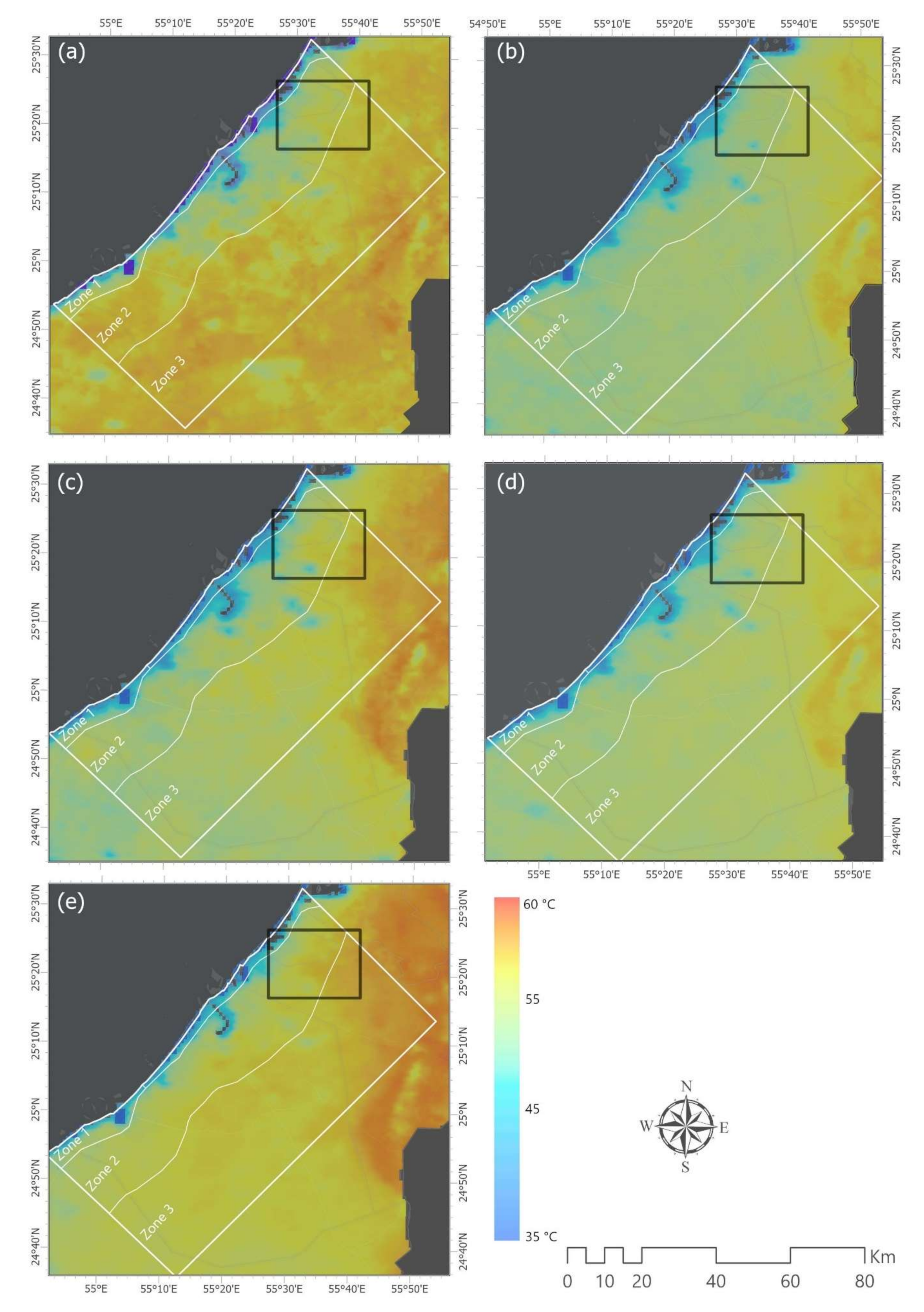
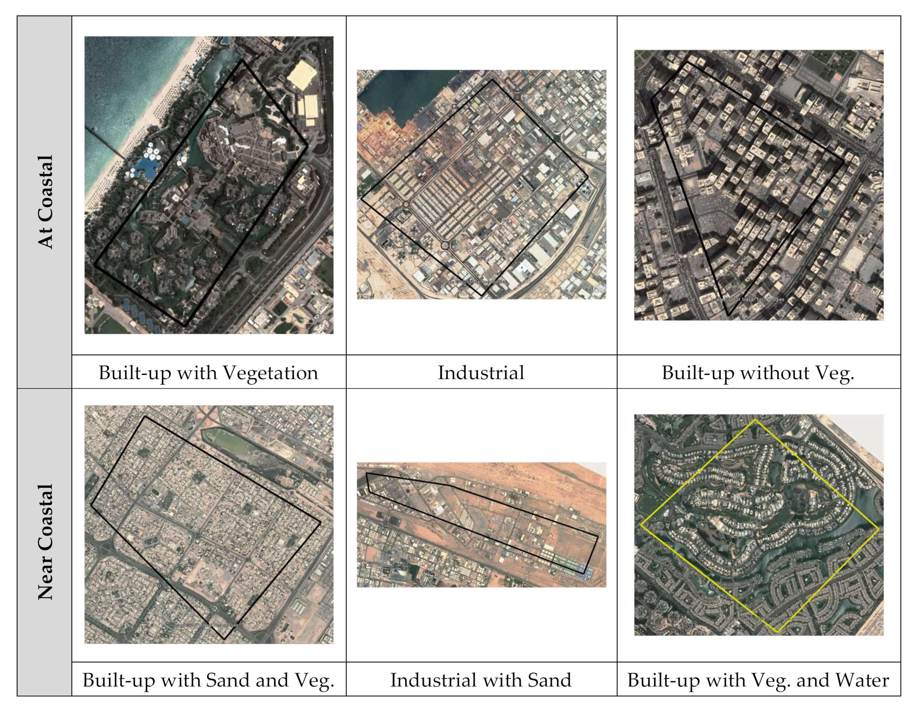
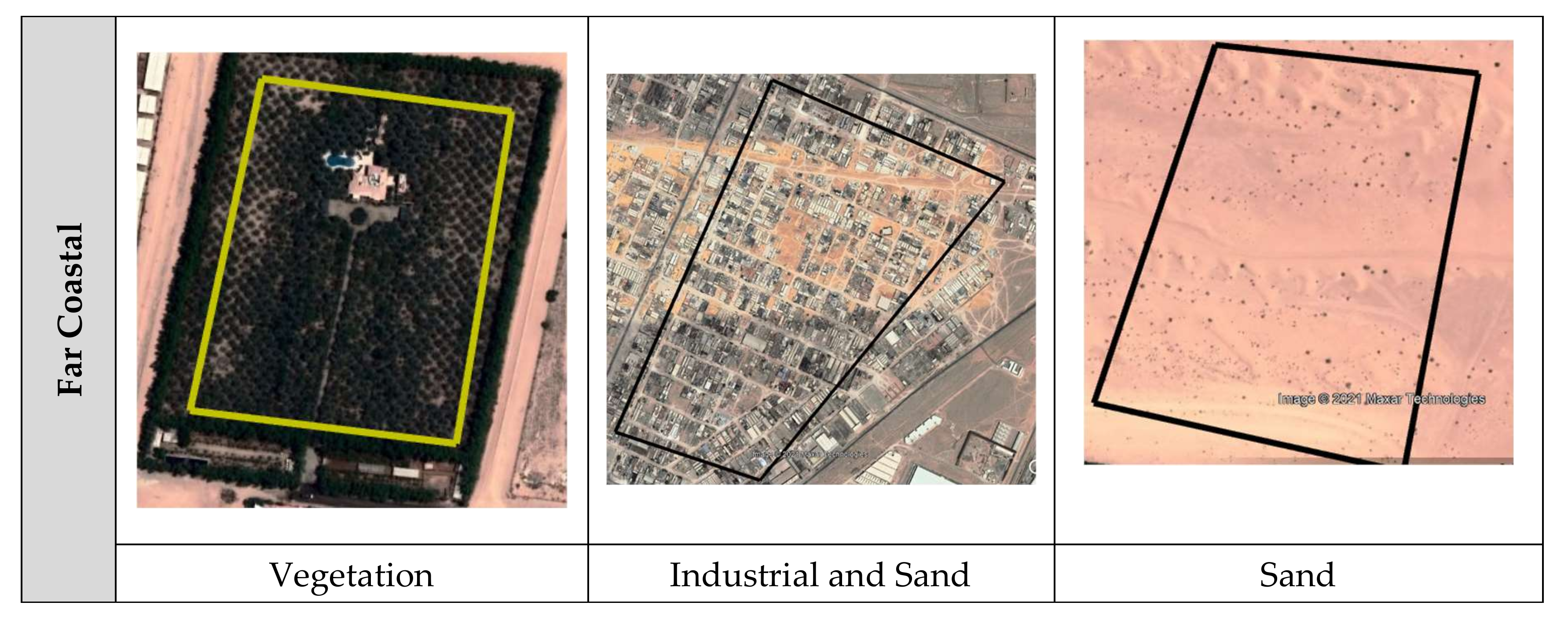
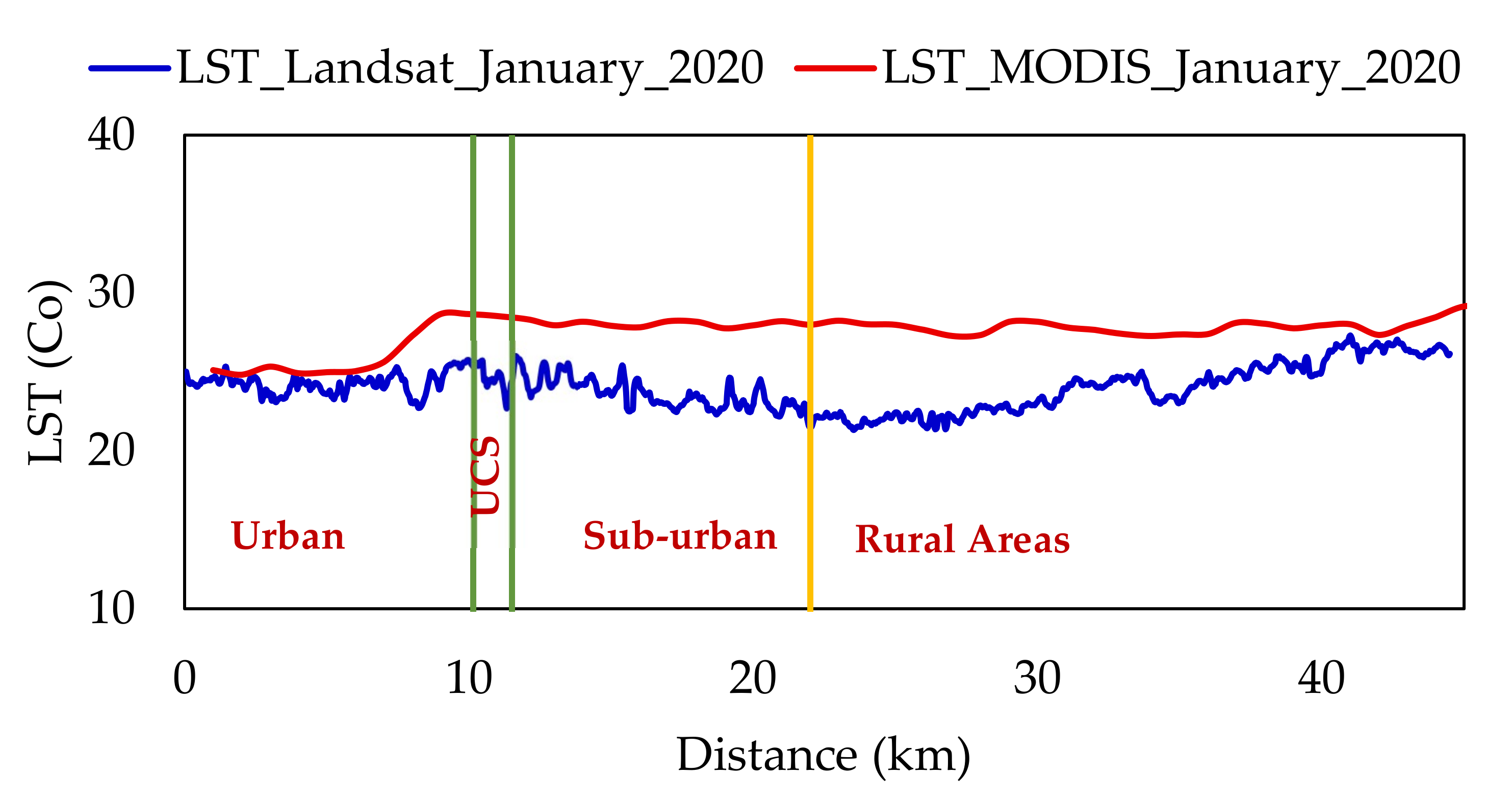
8.1. Spatial Assessment of LST

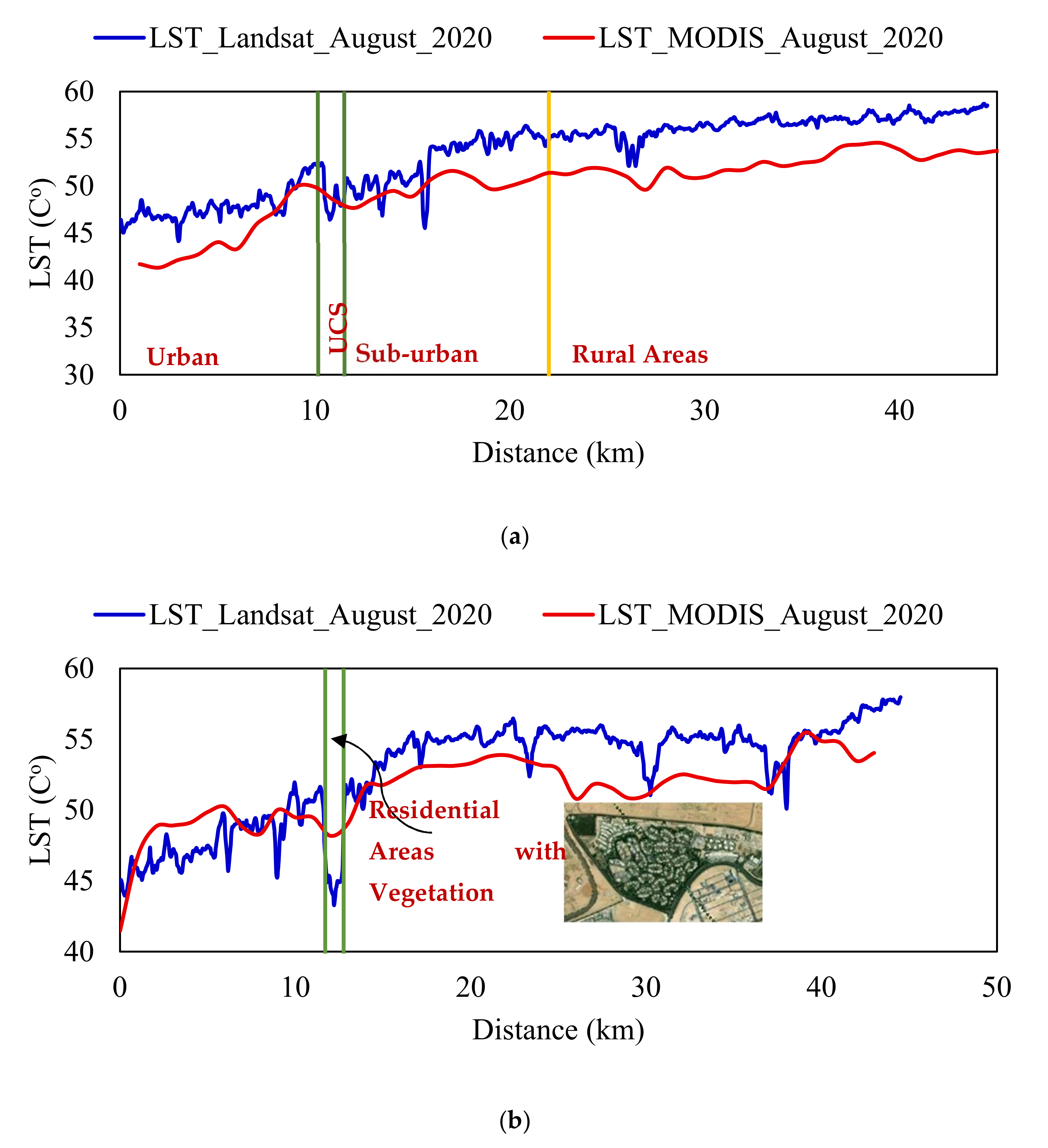
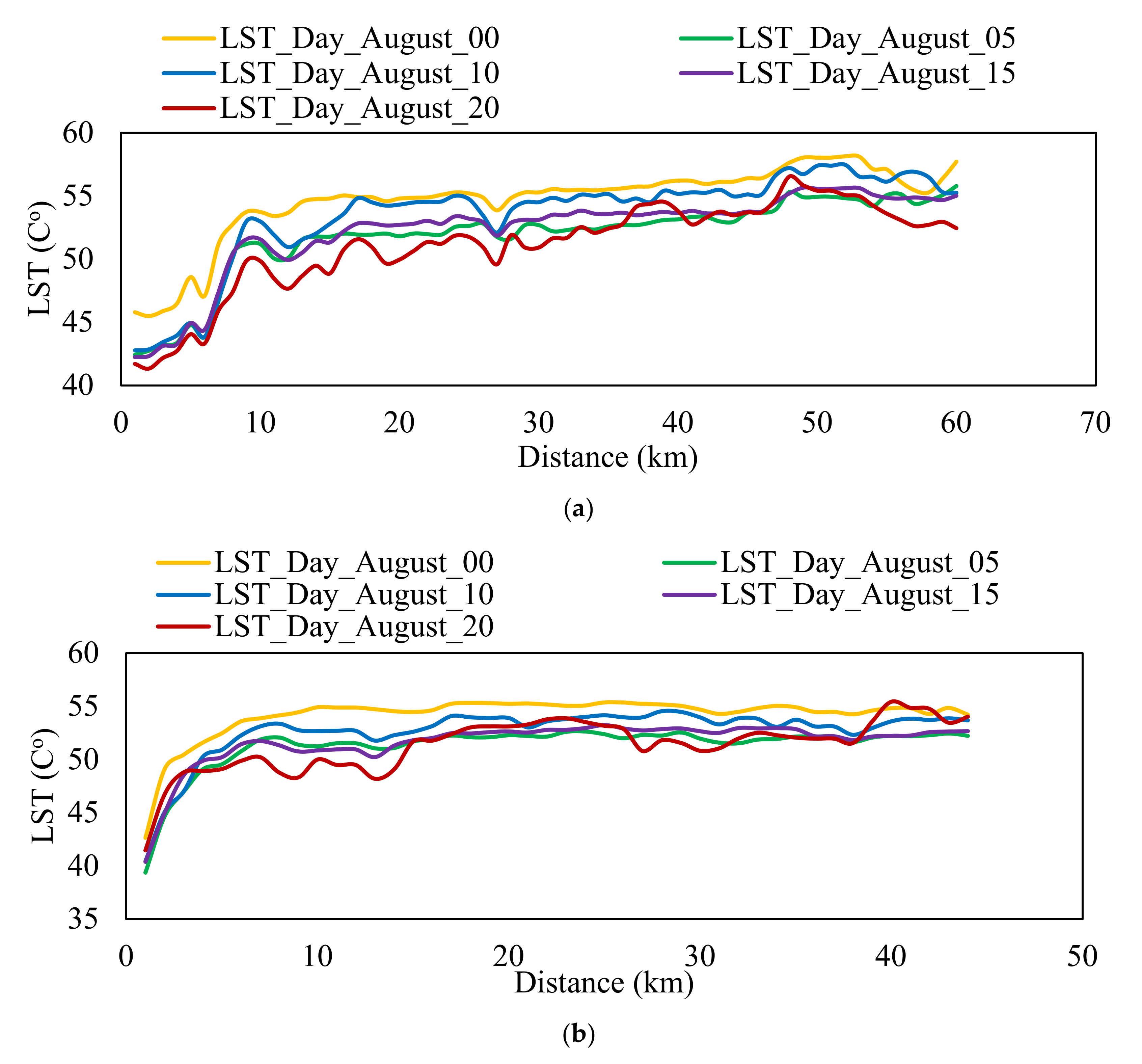
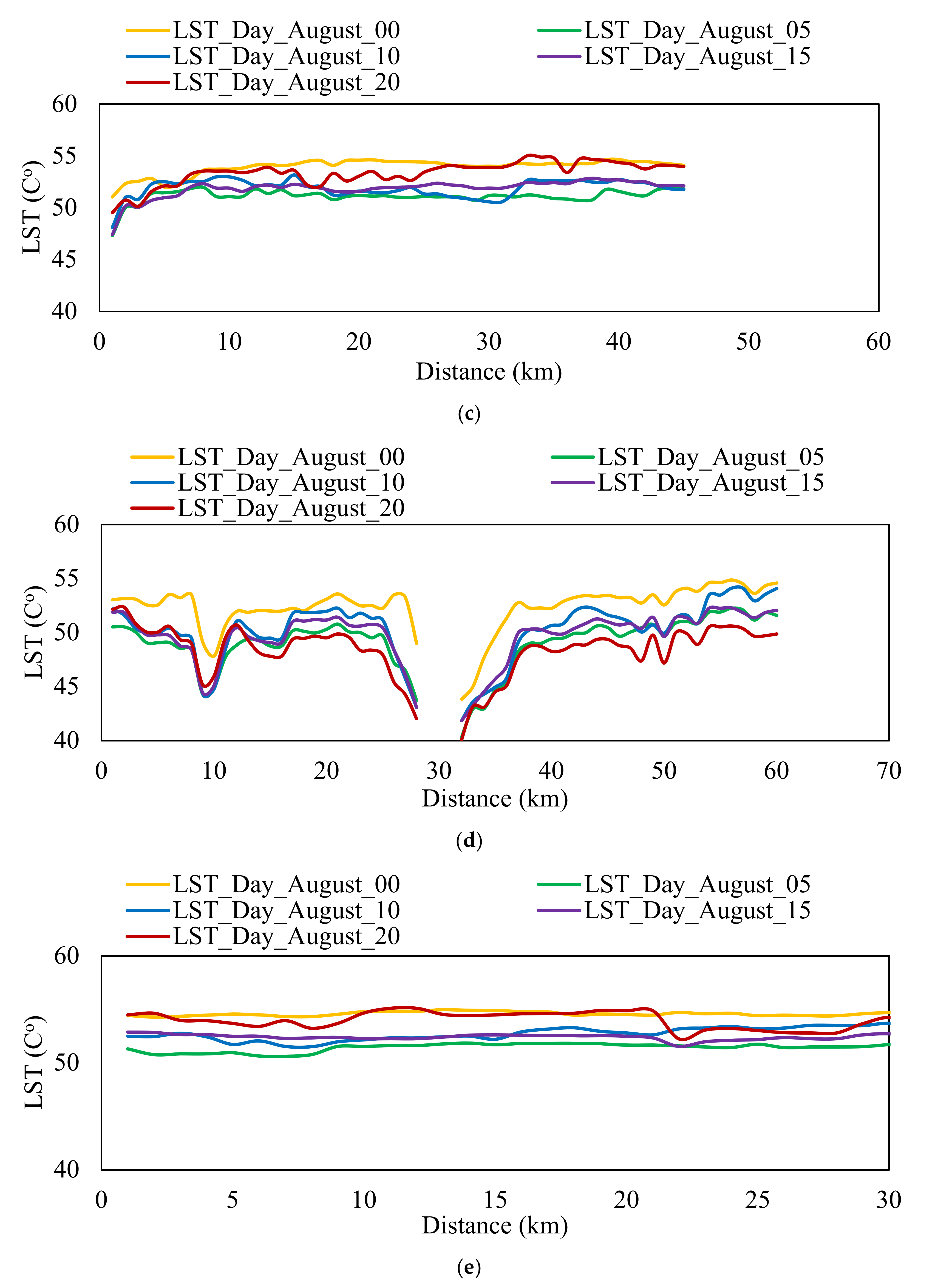
8.1.1. Summer Profiling

In this part, we utilized LST from Landsat satellite images to study the spatial progressions of LST in our study area. Five major profiles were considered, as shown in Figure 12. These profiles consider the following spatial aspects: (i) LST progression from the coast up to rural areas, (ii) LST over the coastline, and (iii) LST in the rural areas. The LST from the Landsat satellite was opted for this analysis, given its higher spatial resolution compared to MODIS images. Nevertheless, we opted to only include the LST result from the MODIS images for comparative purposes. It is important to mention here that we were unable to retrieve a complete LST for the winter season from the Landsat images given the presence of clouds.

Figure 13 shows one retrieved LST from Landsat images for the study area. Overall, we can clearly observe that the temperature near the coastlines is cooler than in the rural areas. One of the potential justifications for this observation is that the urbanization in the study area was partially associated with transforming desert lands into vegetation, which, in its turn, contributes to cooling the LST compared to other untouched areas. Additionally, the extra shading that a high-rise building provides could play a role in cooling the LST. Another essential context to mention here is the effect of the gulf breeze coming from the northwest. As shown previously, our wind pattern analysis showed a significant frequency of wind blowing from the gulf direction during daytime (Section 6) [42,46,47]. This observation is defined as the inverse of UHI, where urban areas are cooler than rural areas [8]. In the following paragraphs, we will explore the LST over each of the profiles above and understand how the LST is changing spatially over the study area.

Figure 14 shows different imposed LST profiling over the study area. As can be observed from Profiles 1 to 3 (Figure 14a–c), the urban area close to the coastline is cooler than the urban area. There are some miscellaneous drops in LST due to a sudden land-use change. For instance, the LST in the residential area with heavy vegetation in Profile 2 dropped suddenly as compared to the surrounding sand areas.

Figure 14d depicts the LST of Profile 4, which runs along the coastline of the study area. As can be seen, the results show a consistent LST ranging between 45 and 53 °C, except at the water body where the LST drops significantly. It is worth highlighting that urbanization in Profile 2 gradually increases along the line until it reaches its maximum towards the end of the profile. Nevertheless, urbanization density does not seem to affect the LST over the coastline significantly.

Figure 14e shows the LST of Profile 5 that runs horizontally in the rural area far from the study area’s coastlines. The LST along this profile was almost consistent with some spikes due to some remotely urban clusters in the profile.

Generally, it is observed here that the significant factors that affected the LST variations were urbanization and the distance from the coastline. Furthermore, the LST from both Landsat and MODIS across the five profiles were partially compatible with each other. In the next paragraph, we will elaborate our analysis by performing zonal statistics to better understand the effect of urbanization and coastlines on LST.

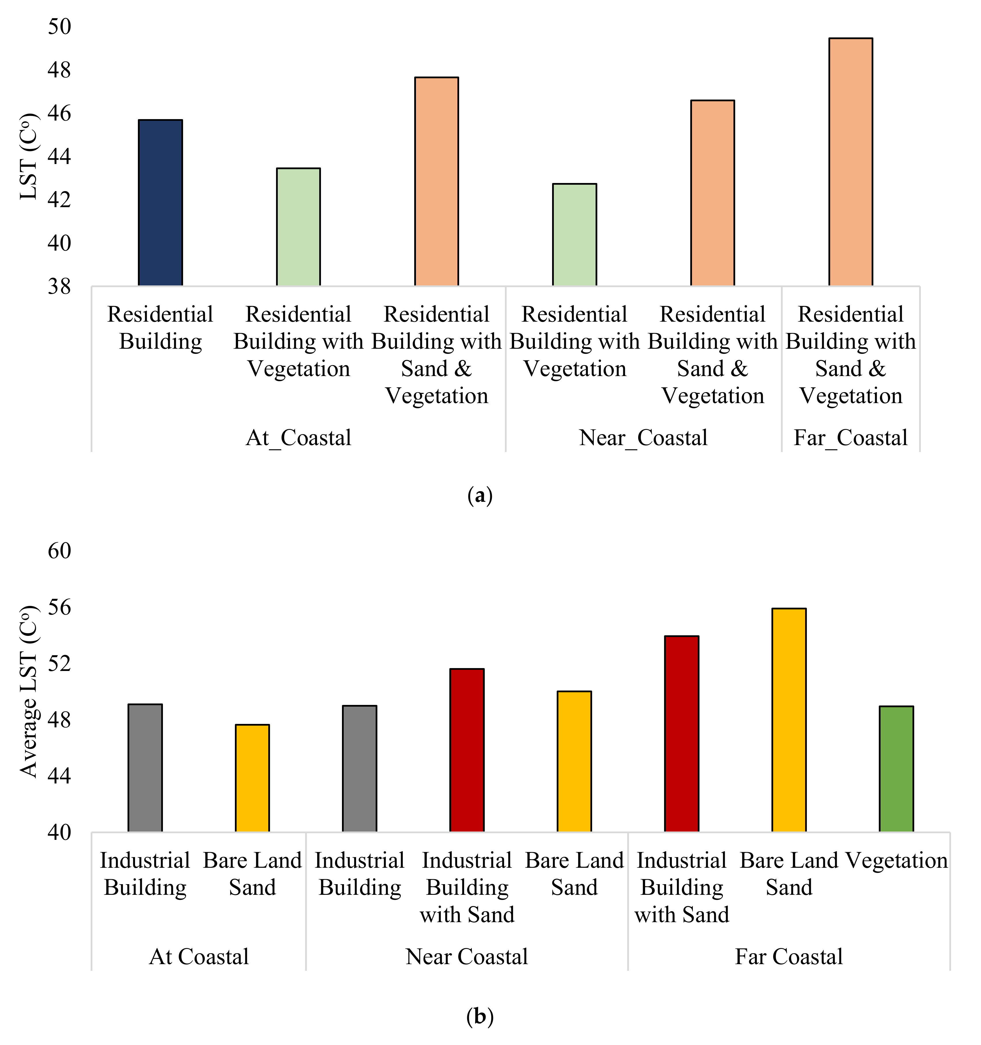
8.1.2. Zonal Statistics

More than 35 zones were selected across the study area with different land use and locations to analyze the zonal statistics. Figure 15 shows close imagery of designated zones. For each selected zone, the average LST of the zone was calculated and then labeled based on the zone’s land use and its location in the study area (i.e., at-coastal, near-coastal, or far-coastal). Figure 16 shows the average LST for the zones selected in the study area. As can be seen, the following points could be concluded:

• The areas of the industrial building have generally higher LST than areas of residential buildings;
• The presence of vegetation in any area, regardless of its proximity distance from the coastline, could reduce the LST;
• The presence of sand in any area, regardless of its proximity distance from the coastline, could increase the LST compared to areas that are fully urbanized (whether industrial or residential buildings);
• The LST of the bare land sand increases as the distance from the coastline increases.

It is important to note that the zonal statistics presented here are a macro-analysis where the LST and land-use classification are executed over a large scale (i.e., Landsat images of 120 m resampled at 30 m). Landsat images’ coarse spatial and temporal resolution (relative to low-range images by Arial or drones) impede the comprehensive comparative analysis between the zones across the different regions. This is because the percentage of urbanization and bare land sand could differ across zones and might be difficult to delineate by Landsat images accurately.

Additionally, we conducted a band correlation analysis to better understand the collaborative relationship between land use and the LST. The study showed that a built-up area (residential and industrial building) negatively correlates with LST by −0.46; the vegetation versus LST is −0.16, and bare land sand versus LST is 0.65. This “macro” correlation indicates that urbanization could decrease the LST during the daytime during the summer season. A clear caveat is that the proportion of areas between the different land uses could affect the strength of the correlation. Nevertheless, the presented analysis indicates the influence of each land use on LST.

8.1.3. Winter Profiling

In winter, however, the LST spatial progression could be different. Figure 17 shows the spatial progression of LST during the winter season in 2020 (especially in January). Contrary to Figure 14a (i.e., daytime LST of Profile 1 in summer), the profile did not show a noticeable change in LST from urban to rural areas. The LST in Profile 1 was consistent at an average LST of about 24 °C. Furthermore, the LST from Landsat and MODIS are partially compatible.

In conclusion, the following points were drawn from examining the spatial progression of the LST in the study area: In summer, the LST in rural areas is higher than in urban centers near the coastline. Compared to other studies in the literature, one would expect the opposite. The inversion phenomenon in this observation could be attributed to the transformation of desert lands into vegetation. Moreover, the shading of the newly constructed high-rise building could play a role in cooling the LST in urban centers. In winter, the LST in rural areas is approximately similar to those in urban areas. The land use affects altering the LST; for instance, the vegetation could decrease the LST. By comparing the LST from Landsat and MODIS, the summer values of both satellites are more compatible in summer than winter. The following section will utilize MODIS images to explore how the LST changed temporally over the study area, i.e., day vs. night and summer vs. winter.

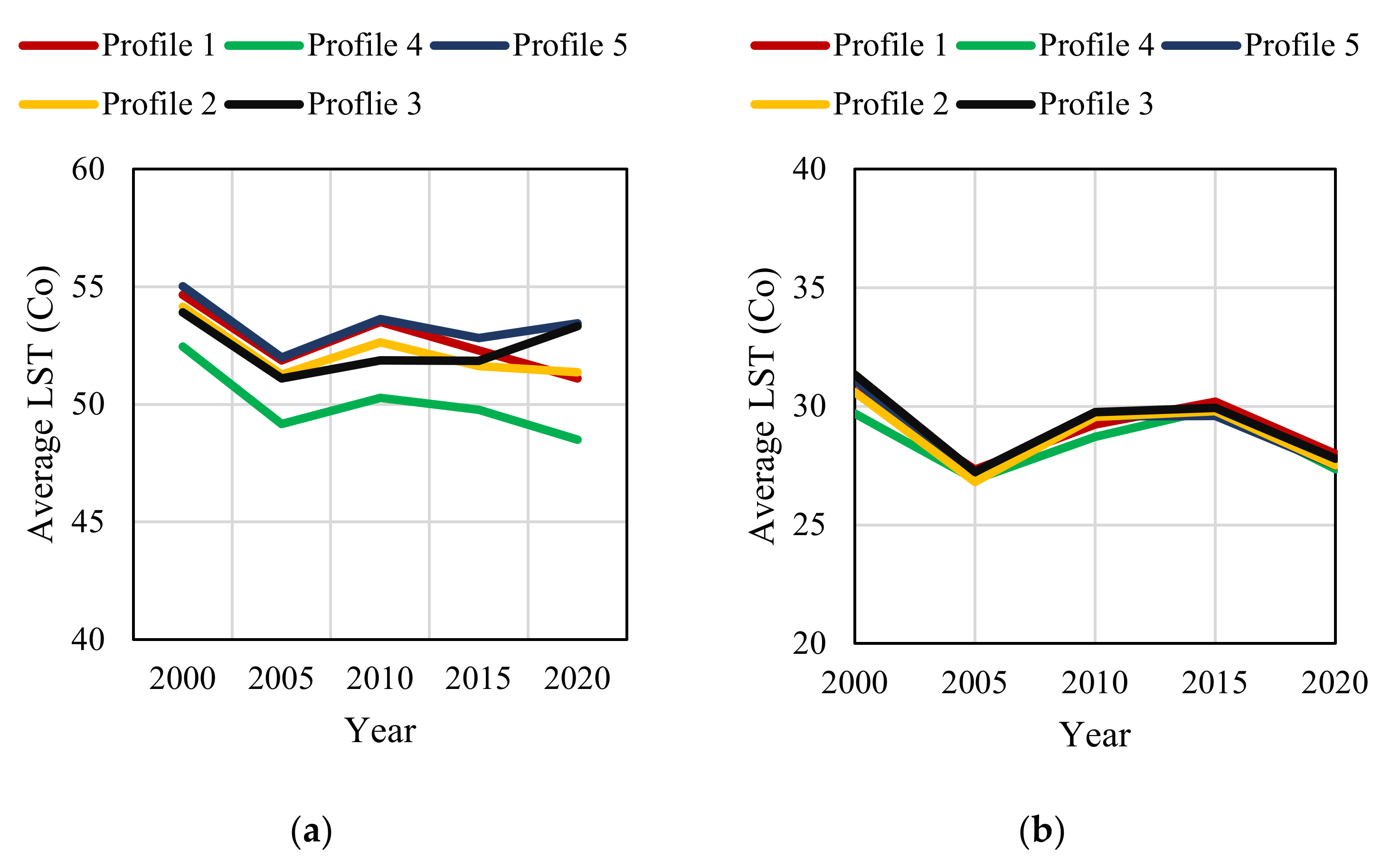
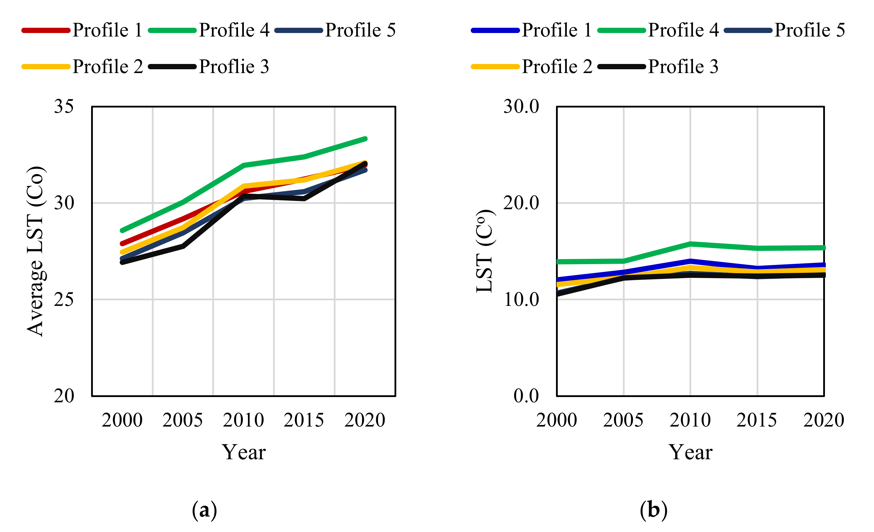
8.2. Temporal Evolution of LST

In this section, the temporal evolution of the LST will be examined for day versus night and summer versus winter. Given the high temporal resolution of the MODIS satellite images, they were used for this analysis as the primary source of data.

8.2.1. Daytime LST

Figure 18 shows the temporal evolutions of daytime LST during the summer seasons. As can be seen, there were some fluctuations in the LST across the five profiles. For instance, the highest yearly LST in Profile 5 was in August 2000, while the lowest was in August 2005, and the other years were in between. A similar analysis was conducted for the daytime LST in the winter seasons (average of January of 2000 until 2020 with a five-year pace). Figure 19 below illustrates the average daytime LST of the five profiles in both seasons to provide a comparative assessment of daytime LST in summer and winter. Overall, the average LST profiles are not exhibiting any clear trend indicating a significant temporal change in LST daytime, neither in summer nor winter.

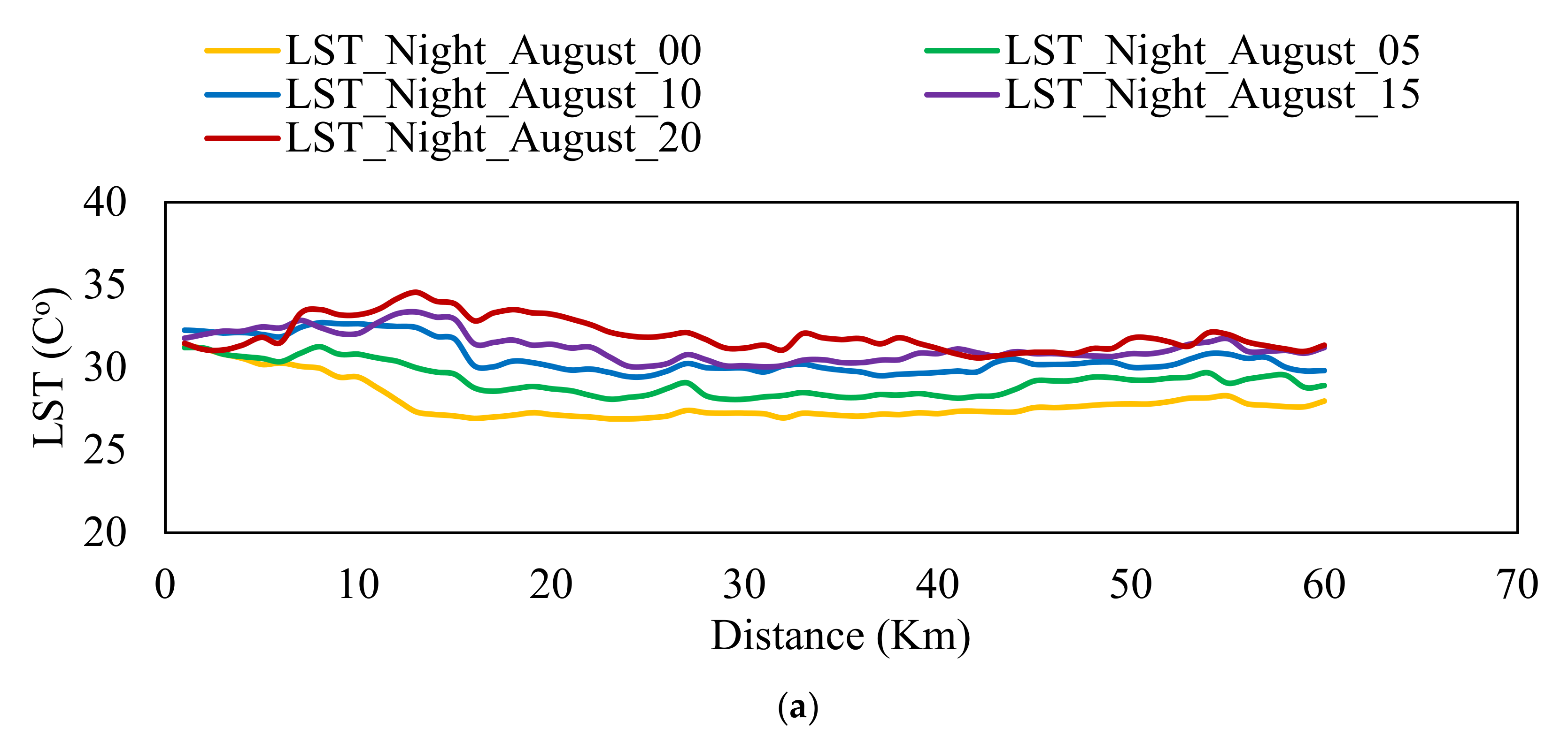
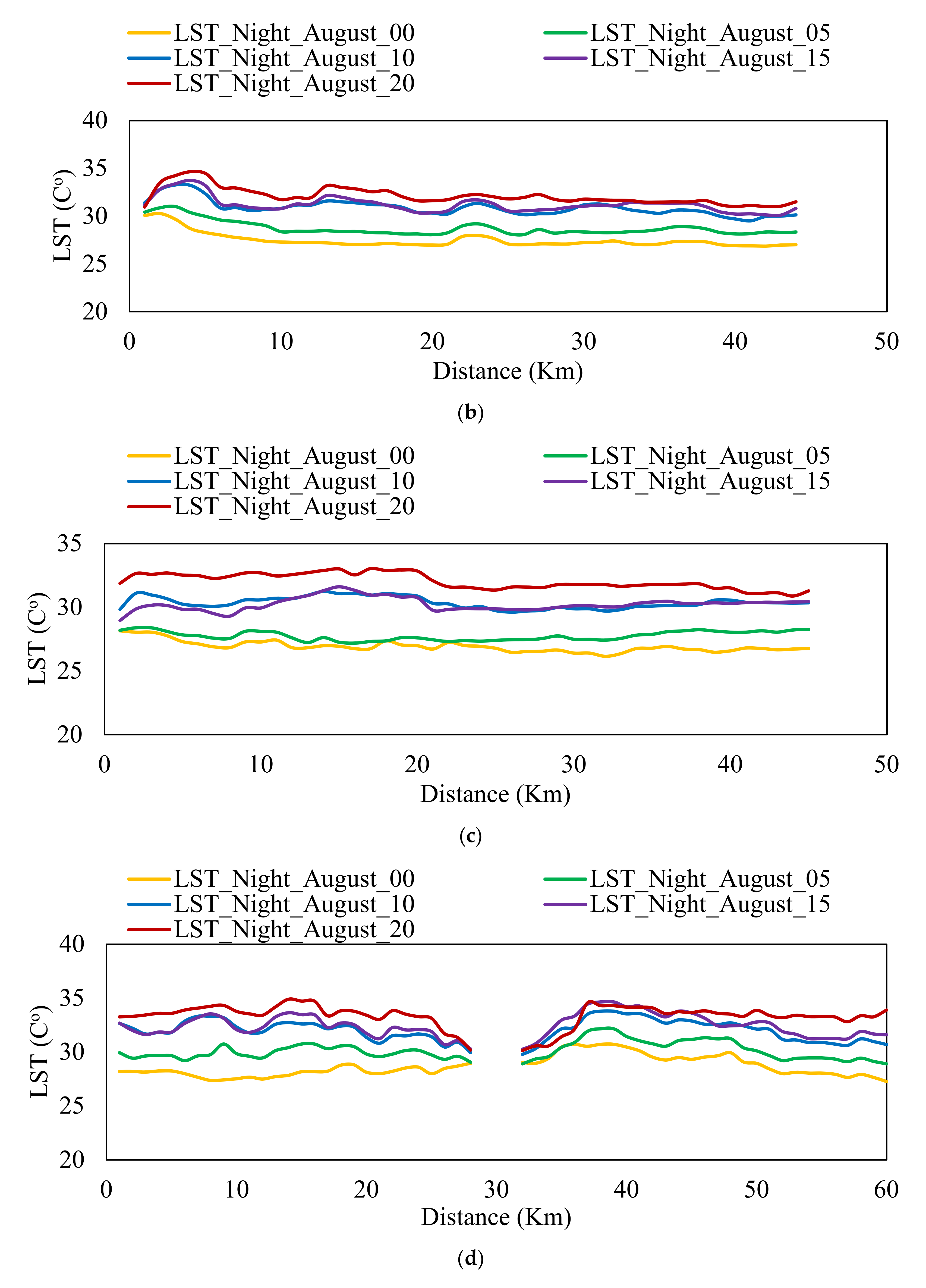
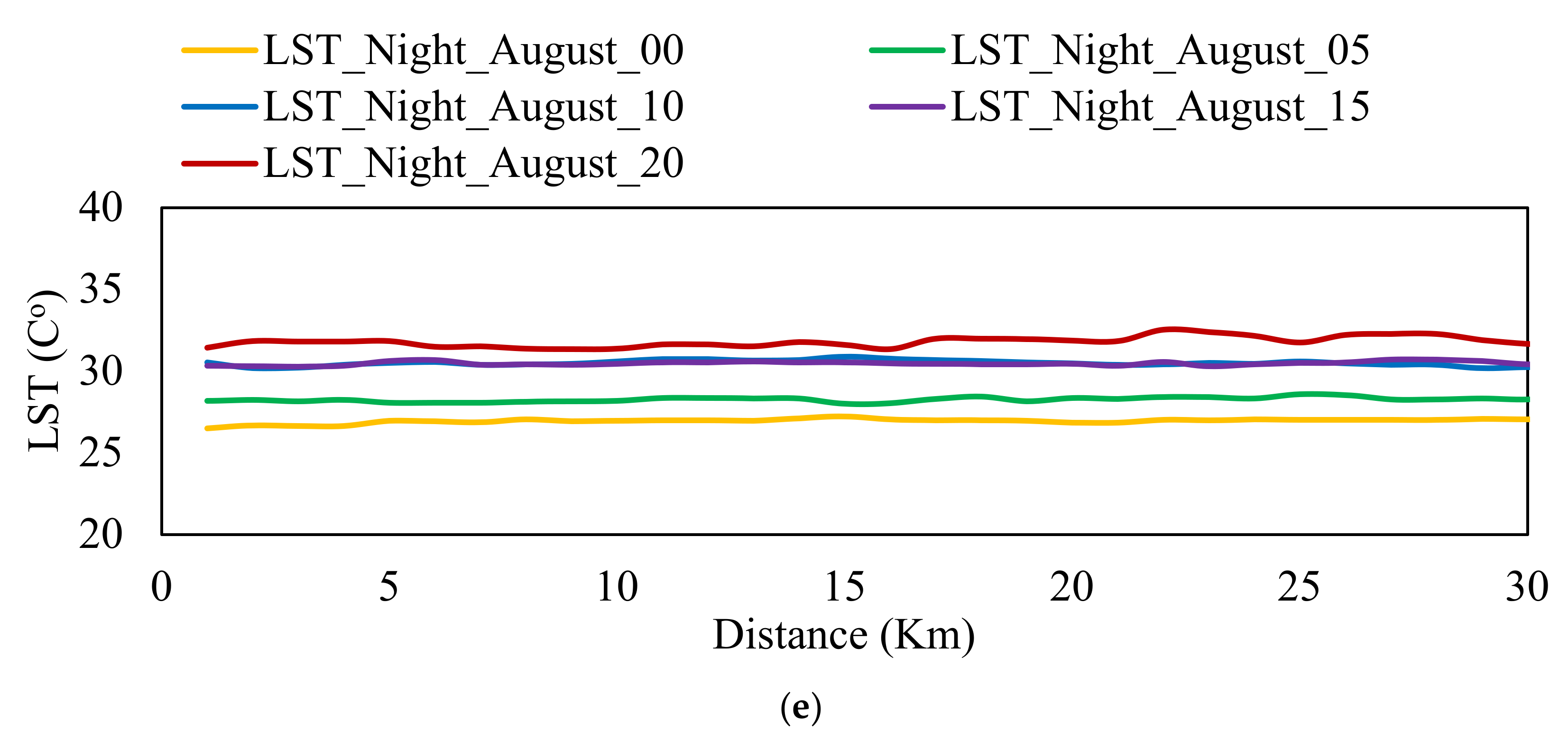
8.2.2. Nighttime LST

To have a deeper understanding of the temporal changes of LST at nighttime, the same three profiles shown in Figure 12 were utilized. Figure 20 presents the LST at nighttime for each profile, as discussed earlier. Figure 20a shows the temporal evolution of Profile 1. In general, the LST increased over the years. There is some indication that the LST of nighttime increases as it moves away from the coast until it reaches the city (at about 20 km from the coastline). After that, the nighttime LST seems to be somehow stable with a slight increase. Figure 20b shows the evolution of Profile 2, which happens to be along the coastline. This profile passes through a water body called Dubai creek. As we approach the creek, the nighttime LST decreases then the trend line continues after it. The same is also observed here in that the nighttime LST increased over the years. However, there are no severe changes along with the profiles themselves in that the average profile for each year is somehow constant. The final shape is shown in Figure 20c, where it was taken far away from the urban city in parallel to the coastline. This profile shows a controlled land use that did not face any significant urbanization. Overall, the LST of the nighttime increases from 2000 up to 2020, with an average increase of 4.6 °C.

Accordingly, a similar analysis was performed for nighttime LST during the winter. To have a comparative assessment of how the nighttime LST changed between summer and winter, Figure 21 shows the average nighttime LST in both seasons (summer: August, and winter: January) for the three profiles shown in Figure 12. As shown in Figure 21a, the nighttime LST increases temporally in the summer seasons. However, the nighttime LST (Figure 21b) is somehow stable temporally in the winter seasons. It is essential to highlight here that the increase in the nighttime LST is compatible with the near-temporal increase in the near-surface temperature illustrated earlier in Section 4. This observation coincides with other studies in the literature that showed that nighttime LST is generally more compatible with near-surface temperature than daytime LST [68,69]. It is important to highlight that the standard deviation ranged between 0.4 and 1.2 °C in 2020.

Overall, the following points could be concluded. In summer, the average daily LST decreases temporally regardless of the land use and the proximity distance from the coastlines. In summer, the average nighttime LST increases temporally regardless of the land use and the proximity distance from the coastlines. In winter, the average nighttime LST is stable temporally and did not exhibit significant changes.

9. Conclusions

This paper investigated the spatial and temporal changes of LST in the day vs. night in the summer and winter seasons in an arid region (major coastal cities of the northern UAE) that has witnessed massive urbanization over the last few decades. Towards that, we utilized satellite images (Landsat and MODIS) to detect the urban changes and the LST. The findings of this paper could be summarized as follows:

• Contrary to the observed UHI in other regions, the LST in our study area increases spatially as we move away from urban areas. This observation could be characterized as a spatial inversion of UHI. The possible reason behind this is that the bare land in the study area is now sand, vegetation, and high-rise buildings, which provide an extra shading to their surrounding area and replaced those bare lands. Moreover, the effect of the gulf breeze coming from the northwest might play a role in cooling the hot air in the urban areas close to the coast, thus, making them cooler than rural areas.
• The analysis of the study did not show any significant changes in the daytime LST, neither in summer nor in winter. At the same time, the nighttime LST increased temporally in the summer seasons by 17% since 2000. Nevertheless, the nighttime LST in the winter seasons showed somehow stable records. This observation could be characterized by the temporal inversion of UHI.
• The zonal statistics of the summer LST showed that areas with industrial buildings have generally higher temperatures than areas with residential buildings. Furthermore, the presence of bare sand in urban areas has a relatively higher LST than in areas that are fully urbanized (facilities with/out vegetation).

Although the results presented in this paper are specific to our study area, the outlined methodology could be implemented in other regions to investigate the LST spatially and temporally using satellite images. For example, the outlined method provides a framework for conducting conventional and high-accuracy urban change detection and retrieving LST maps for any study area. Further, the methodology illustrates how to analyze those LST maps using longitudinal and transverse profiles and highlights the importance of daytime versus nighttime and summer versus winter. The results could inspire other researchers to focus on related details (such as urbanization, vegetation, and sea and land breeze) to explain the LST in their study area. All of this will provide valuable information to decision-makers and engineers concerned with maintaining a high quality of life while developing the new urban areas of their cities.

References

- Liu, Z.; Wang, Y.; Li, Z.; Peng, J. Impervious surface impact on water quality in the process of rapid urbanization in Shenzhen, China. Environ. Earth Sci. 2013, 68, 2365–2373. [Google Scholar] [CrossRef]
- Nelken, K.; Leziak, K. The seasonal variability of the amount of global solar radiation reaching the ground in urban and rural areas on the example of Warsaw and Belsk. Misc. Geogr. 2016, 20, 29–37. [Google Scholar] [CrossRef] [Green Version]
- Robaa, S.M. A study of ultraviolet solar radiation at Cairo urban area, Egypt. Sol. Energy 2004, 77, 251–259. [Google Scholar] [CrossRef]
- Robaa, S.M. Urban-rural solar radiation loss in the atmosphere of Greater Cairo region, Egypt. Energy Convers. Manag. 2009, 50, 194–202. [Google Scholar] [CrossRef]
- Park, H.-S. Features of the heat island in seoul and its surrounding cities. Atmos. Environ. 1986, 20, 1859–1866. [Google Scholar] [CrossRef]
- Middel, A.; Brazel, A.J.; Kaplana, S.; Myint, S.W. Daytime cooling efficiency and diurnal energy balance in Phoenix, Arizona, USA. Clim. Res. 2012, 54, 21–34. [Google Scholar] [CrossRef] [Green Version]
- Kato, S.; Yamaguchi, Y. Estimation of storage heat flux in an urban area using ASTER data. Remote Sens. Environ. 2007, 110, 1–17. [Google Scholar] [CrossRef]
- Lazzarini, M.; Marpu, P.R.; Ghedira, H. Temperature-land cover interactions: The inversion of urban heat island phenomenon in desert city areas. Remote Sens. Environ. 2013, 130, 136–152. [Google Scholar] [CrossRef]
- Rivera, E.; Antonio-Némiga, X.; Origel-Gutiérrez, G.; Sarricolea, P.; Adame-Martínez, S. Spatiotemporal analysis of the atmospheric and surface urban heat islands of the Metropolitan Area of Toluca, Mexico. Environ. Earth Sci. 2017, 76, 1–14. [Google Scholar] [CrossRef]
- Schwarz, N.; Lautenbach, S.; Seppelt, R. Exploring indicators for quantifying surface urban heat islands of European cities with MODIS land surface temperatures. Remote Sens. Environ. 2011, 115, 3175–3186. [Google Scholar] [CrossRef]
- Phelan, P.E.; Kaloush, K.; Miner, M.; Golden, J.; Phelan, B.; Silva, H., III; Taylor, R.A. Urban Heat Island: Mechanisms, Implications, and Possible Remedies. Annu. Rev. Environ. Resour. 2015, 40, 285–307. [Google Scholar] [CrossRef]
- Rizwan, A.M.; Dennis, L.Y.; Chunho, L.I.U. A review on the generation, determination and mitigation of Urban Heat Island. J. Environ. Sci. 2008, 20, 120–128. [Google Scholar] [CrossRef]
- Amirtham, L.R. Urbanization and its impact on urban heat Island intensity in Chennai Metropolitan Area, India. Indian J. Sci. Technol. 2016, 9, 1–8. [Google Scholar] [CrossRef] [Green Version]
- Thomas, G.; Zachariah, E. Urban Heat Island in a Tropical City Interlaced by Wetlands. J. Environ. Sci. 2011, 5, 234–240. [Google Scholar]
- Yao, R.; Wang, L.; Gui, X.; Zheng, Y.; Zhang, H.; Huang, X. Urbanization effects on vegetation and surface urban heat islands in China’s Yangtze River Basin. Remote Sens. 2017, 9, 540. [Google Scholar] [CrossRef] [Green Version]
- Li, G.; Zhang, X.; Mirzaei, P.A.; Zhang, J.; Zhao, Z. Urban heat island effect of a typical valley city in China: Responds to the global warming and rapid urbanization. Sustain. Cities Soc. 2018, 38, 736–745. [Google Scholar] [CrossRef]
- Su, Y.F.; Foody, G.M.; Cheng, K.S. Spatial non-stationarity in the relationships between land cover and surface temperature in an urban heat island and its impacts on thermally sensitive populations. Landsc. Urban Plan. 2012, 107, 172–180. [Google Scholar] [CrossRef]
- Coseo, P.; Larsen, L. Accurate characterization of land cover in urban environments: Determining the importance of including obscured impervious surfaces in urban heat island models. Atmosphere 2019, 10, 347. [Google Scholar] [CrossRef] [Green Version]
- Chen, T.; Sun, A.; Niu, R. Effect of land cover fractions on changes in surface urban heat islands using landsat time-series images. Int. J. Environ. Res. Public Health 2019, 16, 971. [Google Scholar] [CrossRef] [Green Version]
- Li, B.; Liu, Z.; Nan, Y.; Li, S.; Yang, Y. Comparative analysis of urban heat island intensities in Chinese, Russian, and DPRK regions across the transnational urban agglomeration of the Tumen River in Northeast Asia. Sustainability 2018, 10, 2637. [Google Scholar] [CrossRef] [Green Version]
- Filho, W.L.; Icaza, L.E.; Emanche, V.O.; Al-Amin, A.Q. An evidence-based review of impacts, strategies and tools to mitigate urban heat islands. Int. J. Environ. Res. Public Health 2017, 14, 1600. [Google Scholar] [CrossRef] [PubMed] [Green Version]
- Beaudoin, M.; Gosselin, P. An effective public health program to reduce urban heat islands in Québec, Canada. Rev. Panam. Salud Publica/Pan Am. J. Public Health 2016, 40, 160–166. [Google Scholar]
- Van Der Hoeven, F.; Wandl, A. Amsterwarm: Mapping the landuse, health and energy-efficiency implications of the Amsterdam urban heat island. Build. Serv. Eng. Res. Technol. 2015, 36, 67–88. [Google Scholar] [CrossRef]
- Che-Ani, A.I.; Shahmohamadi, P.; Sairi, A.; Mohd-Nor, M.F.I.; Zain, M.F.M.; Surat, M. Mitigating the urban heat island effect: Some points without altering existing city planning. Eur. J. Sci. Res. 2009, 35, 204–216. [Google Scholar]
- Debbage, N.; Shepherd, J.M. The urban heat island effect and city contiguity. Comput. Environ. Urban Syst. 2015, 54, 181–194. [Google Scholar] [CrossRef]
- Sharma, R.; Joshi, P.K. Identifying seasonal heat islands in urban settings of Delhi (India) using remotely sensed data—An anomaly based approach. Urban Clim. 2014, 9, 19–34. [Google Scholar] [CrossRef]
- Bokaie, M.; Zarkesh, M.K.; Arasteh, P.D.; Hosseini, A. Assessment of Urban Heat Island based on the relationship between land surface temperature and Land Use/Land Cover in Tehran. Sustain. Cities Soc. 2016, 23, 94–104. [Google Scholar] [CrossRef]
- Mathew, A.; Khandelwal, S.; Kaul, N. Analysis of diurnal surface temperature variations for the assessment of surface urban heat island effect over Indian cities. Energy Build. 2018, 159, 271–295. [Google Scholar] [CrossRef]
- Cristóbal, J.; Jiménez-Muñoz, J.C.; Sobrino, J.A.; Ninyerola, M.; Pons, X. Improvements in land surface temperature retrieval from the Landsat series thermal band using water vapor and air temperature. J. Geophys. Res. Atmos. 2009, 114, 1–16. [Google Scholar] [CrossRef]
- Kafer, P.S.; Rolim, S.B.A.; Iglesias, M.L.; da Rocha, N.S.; Diaz, L.R. Land Surface Temperature Retrieval by LANDSAT 8 Thermal Band: Applications of Laboratory and Field Measurements. IEEE J. Sel. Top. Appl. Earth Obs. Remote Sens. 2019, 12, 2332–2341. [Google Scholar] [CrossRef]
- Li, F.; Jackson, T.J.; Kustas, W.P.; Schmugge, T.J.; French, A.N.; Cosh, M.H.; Bindlish, R. Deriving land surface temperature from Landsat 5 and 7 during SMEX02/SMACEX. Remote Sens. Environ. 2004, 92, 521–534. [Google Scholar] [CrossRef]
- Gui, X.; Wang, L.; Yao, R.; Yu, D.; Li, C. Investigating the urbanization process and its impact on vegetation change and urban heat island in Wuhan, China. Environ. Sci. Pollut. Res. 2019, 26, 30808–30825. [Google Scholar] [CrossRef] [PubMed]
- Katpatal, Y.B.; Kute, A.; Satapathy, D.R. Surface- and air-temperature studies in relation to land use/land cover of nagpur urban area using landsat 5 TM data. J. Urban Plan. Dev. 2008, 134, 110–118. [Google Scholar] [CrossRef]
- Kotharkar, R.; Bagade, A. Evaluating urban heat island in the critical local climate zones of an Indian city. Landsc. Urban Plan. 2018, 169, 92–104. [Google Scholar] [CrossRef]
- Mohammad, P.; Goswami, A.; Bonafoni, S. The impact of the land cover dynamics on surface urban heat island variations in semi-arid cities: A case study in Ahmedabad City, India, using multi-sensor/source data. Sensors 2019, 19, 3701. [Google Scholar] [CrossRef] [PubMed] [Green Version]
- Ochola, E.M.; Fakharizadehshirazi, E.; Adimo, A.O.; Mukundi, J.B.; Wesonga, J.M.; Sodoudi, S. Inter-local climate zone differentiation of land surface temperatures for Management of Urban Heat in Nairobi City, Kenya. Urban Clim. 2020, 31, 100540. [Google Scholar] [CrossRef]
- Qiao, Z.; Liu, L.; Qin, Y.; Xu, X.; Wang, B.; Liu, Z. The impact of urban renewal on land surface temperature changes: A case study in the main city of Guangzhou, China. Remote Sens. 2020, 12, 794. [Google Scholar] [CrossRef] [Green Version]
- Golden, J.S.; Kaloush, K.E. Mesoscale and microscale evaluation of surface pavement impacts on the urban heat island effects. Int. J. Pavement Eng. 2006, 7, 37–52. [Google Scholar] [CrossRef]
- Abulibdeh, A. Analysis of urban heat island characteristics and mitigation strategies for eight arid and semi-arid gulf region cities. Environ. Earth Sci. 2021, 80, 1–26. [Google Scholar] [CrossRef]
- Mohamed, M.; Othman, A.; Abotalib, A.Z.; Majrashi, A. Urban heat island effects on megacities in desert environments using spatial network analysis and remote sensing data: A case study from western Saudi Arabia. Remote Sens. 2021, 13, 1941. [Google Scholar] [CrossRef]
- Bala, R.; Prasad, R.; Pratap Yadav, V. A comparative analysis of day and night land surface temperature in two semi-arid cities using satellite images sampled in different seasons. Adv. Sp. Res. 2020, 66, 412–425. [Google Scholar] [CrossRef]
- He, B.J. Potentials of meteorological characteristics and synoptic conditions to mitigate urban heat island effects. Urban Clim. 2018, 24, 26–33. [Google Scholar] [CrossRef]
- Sakakibara, Y.; Matsui, E. Relation between heat island intensity and city size indices/urban canopy characteristics in settlements of Nagano basin, Japan. Geogr. Rev. Jpn. 2005, 78, 812–824. [Google Scholar] [CrossRef] [Green Version]
- Zak, M.; Nita, I.A.; Dumitrescu, A.; Cheval, S. Influence of synoptic scale atmospheric circulation on the development of urban heat island in Prague and Bucharest. Urban Clim. 2020, 34, 100681. [Google Scholar] [CrossRef]
- He, B.J.; Wang, J.; Liu, H.; Ulpiani, G. Localized synergies between heat waves and urban heat islands: Implications on human thermal comfort and urban heat management. Environ. Res. 2021, 193, 110584. [Google Scholar] [CrossRef]
- He, B.J.; Ding, L.; Prasad, D. Relationships among local-scale urban morphology, urban ventilation, urban heat island and outdoor thermal comfort under sea breeze influence. Sustain. Cities Soc. 2020, 60, 102289. [Google Scholar] [CrossRef]
- He, B.J.; Ding, L.; Prasad, D. Wind-sensitive urban planning and design: Precinct ventilation performance and its potential for local warming mitigation in an open midrise gridiron precinct. J. Build. Eng. 2020, 29, 101145. [Google Scholar] [CrossRef]
- Khalil, M.; Al-Ruzouq, R.; Hamad, K.; Shanableh, A. Multi-Temporal satellite imagery for infrastructure growth assessment of Dubai City, UAE. In Proceedings of the MATEC Web of Conferences, Sharjah, United Arab Emirates, 18–20 April 2017; Volume 120, p. 09006. [Google Scholar]
- Nassar, A.K.; Alan Blackburn, G.; Duncan Whyatt, J. Developing the desert: The pace and process of urban growth in Dubai. Comput. Environ. Urban Syst. 2014, 45, 50–62. [Google Scholar] [CrossRef] [Green Version]
- Al-Ruzouq, R.; Hamad, K.; Shanableh, A.; Khalil, M. Infrastructure growth assessment of urban areas based on multi-temporal satellite images and linear features. Ann. GIS 2017, 23, 183–201. [Google Scholar] [CrossRef]
- Al-Ruzouq, R.; Yilmaz, A.G.; Shanableh, A.; Boharoun, Z.A.; Khalil, M.A.; Imteaz, M.A. Spatio-temporal analysis of urban growth and its impact on floods in Ajman City, UAE. Environ. Monit. Assess. 2019, 191, 1–21. [Google Scholar] [CrossRef]
- O’Donnell, E.M.; Schott, J.R.; Raqueno, N.G. Calibration history of Landsat thermal data. Int. Geosci. Remote Sens. Symp. 2002, 1, 27–29. [Google Scholar] [CrossRef]
- Barsi, J.A.; Schott, J.R.; Palluconi, F.D.; Helder, D.L.; Hook, S.J.; Markham, B.L.; Chander, G.; O’ Donnell, E.M. Landsat TM and ETM+ thermal band calibration. Can. J. Remote Sens. 2003, 29, 141–153. [Google Scholar] [CrossRef]
- Koutsias, N.; Pleniou, M. Comparing the spectral signal of burned surfaces between Landsat 7 ETM+ and Landsat 8 OLI sensors. Int. J. Remote Sens. 2015, 36, 3714–3732. [Google Scholar] [CrossRef]
- Gibril, M.B.A.; Bakar, S.A.; Yao, K.; Idrees, M.O.; Pradhan, B. Fusion of RADARSAT-2 and multispectral optical remote sensing data for LULC extraction in a tropical agricultural area. Geocarto Int. 2017, 32, 735–748. [Google Scholar] [CrossRef]
- Gibril, M.B.A.; Kalantar, B.; Al-Ruzouq, R.; Ueda, N.; Saeidi, V.; Shanableh, A.; Mansor, S.; Shafri, H.Z.M. Mapping heterogeneous urban landscapes from the fusion of digital surface model and unmanned aerial vehicle-based images using adaptive multiscale image segmentation and classification. Remote Sens. 2020, 12, 1081. [Google Scholar] [CrossRef] [Green Version]
- Hamedianfar, A.; Barakat, A.; Gibril, M. Large-scale urban mapping using integrated geographic object-based image analysis and artificial bee colony optimization from worldview-3 data. Int. J. Remote Sens. 2019, 40, 6796–6821. [Google Scholar] [CrossRef]
- Gibril, M.B.A.; Idrees, M.O.; Yao, K.; Shafri, H.Z.M. Integrative image segmentation optimization and machine learning approach for high quality land-use and land-cover mapping using multisource remote sensing data. J. Appl. Remote Sens. 2018, 12, 016036. [Google Scholar] [CrossRef]
- Hamedianfar, A.; Gibril, M.B.A.; Pellikka, P.K.E. Synergistic use of particle swarm optimization, artificial neural network, and extreme gradient boosting algorithms for urban LULC mapping from WorldView-3 images. Geocarto Int. 2020, 1–19. [Google Scholar] [CrossRef]
- Al-ruzouq, R.; Shanableh, A.; Mohamed, B.; Kalantar, B. Multi-scale correlation-based feature selection and random forest classification for LULC mapping from the integration of SAR and optical Sentinel imagess. In Remote Sensing Technologies and Applications in Urban Environments IV; International Society for Optics and Photonics: Washington, DC, USA, 2019. [Google Scholar] [CrossRef]
- Rouse Junior, J.W.; Hass, R.H.; Schell, J.A.; Deering, D.W. Monitoring vegetation systems in the Great Plains with ERTS. Third Earth Resour. Technol. Satell. Symp. 1974, 1, 309–317. [Google Scholar]
- McFeeters, S.K. The use of the Normalized Difference Water Index (NDWI) in the delineation of open water features. Int. J. Remote Sens. 1996, 17, 1425–1432. [Google Scholar] [CrossRef]
- Zha, Y.; Gao, J.; Ni, S. Use of normalized difference built-up index in automatically mapping urban areas from TM imagery. Int. J. Remote Sens. 2003, 24, 583–594. [Google Scholar] [CrossRef]
- Huete, A.R. A soil-adjusted vegetation index (SAVI). Remote Sens. Environ. 1988, 25, 295–309. [Google Scholar] [CrossRef]
- Ermida, S.L.; Soares, P.; Mantas, V.; Göttsche, F.M.; Trigo, I.F. Google earth engine open-source code for land surface temperature estimation from the landsat series. Remote Sens. 2020, 12, 1471. [Google Scholar] [CrossRef]
- Williamson, S.N.; Hik, D.S.; Gamon, J.A.; Jarosch, A.H.; Anslow, F.S.; Clarke, G.K.C.; Scott Rupp, T. Spring and summer monthly MODIS LST is inherently biased compared to air temperature in snow covered sub-Arctic mountains. Remote Sens. Environ. 2017, 189, 14–24. [Google Scholar] [CrossRef]
- Alqasemi, A.S.; Hereher, M.E.; Al-Quraishi, A.M.F.; Saibi, H.; Aldahan, A.; Abuelgasim, A. Retrieval of monthly maximum and minimum air temperature using MODIS aqua land surface temperature data over the United Arab Emirates. Geocarto Int. 2020, 1–18. [Google Scholar] [CrossRef]
- Sheng, L.; Tang, X.; You, H.; Gu, Q.; Hu, H. Comparison of the urban heat island intensity quantified by using air temperature and Landsat land surface temperature in Hangzhou, China. Ecol. Indic. 2017, 72, 738–746. [Google Scholar] [CrossRef]
- Good, E.J.; Ghent, D.J.; Bulgin, C.E.; Remedios, J.J. A spatiotemporal analysis of the relationship between near-surface air temperature and satellite land surface temperatures using 17 years of data from the ATSR series. J. Geophys. Res. Atmos. 2017, 122, 9185–9210. [Google Scholar] [CrossRef]